Tidal Disruption of a Star By a Massive Black Hole
Computed In Fermi Normal Coordinates
Roseanne M. Cheng
A dissertation submitted to the faculty of the University of North Carolina at Chapel
Hill in partial fulfillment of the requirements for the degree of Doctor of Philosophy
in the Department of Physics and Astronomy.
Chapel Hill
2012
Approved by:
Charles R. Evans
Y. Jack Ng
John Blondin
Jon Engel
Chris Clemens
c
Abstract
ROSEANNE M. CHENG:Tidal Disruption of a Star By a Massive Black Hole Computed In Fermi Normal Coordinates.
(Under the direction of Charles R. Evans.)
We present a new numerical code constructed to obtain accurate simulations of encounters
be-tween a star and a massive black hole. We assume Newtonian hydrodynamics and self-gravity for the
star. The three-dimensional parallel code includes a PPMLR hydrodynamics module to treat the
gas dynamics and a Fourier transform-based method to calculate the self-gravity. The formalism for
calculating the relativistic tidal interaction inFermi normal coordinates (FNC) allows the addition
of an arbitrary number of terms in the tidal expansion. We present the relevant post-Newtonian
terms for this code. Results are given for ann= 1.5 polytrope with comparisons between simulations
and predictions from the linear theory of tidal encounters. It is shown that the inclusion of thel= 3
tidal term will cause the center of mass of the star to deviate from the origin of the FNC. We consider
relativistic encounters for three different mass ratios,µ= 1.28×10−3,4.21
×10−4,3.77
×10−5. We
show a relativistic suppression in the amount of energy deposited onto the star. We find that the
dimensionless functionT2(η) (which characterizes the energy deposited into non-radial oscillations)
must not only be a function of the dimensionless disruption parameter,η, but also of a dimensionless
relativistic parameter Φp. We speculate on the source of the observed energy excess in the tidal
en-counter simulations from the linear theory. We find that the energy deposited into radial oscillations
is negligible and that the shock heating in the outer layers of the post-encounter star contributes a
significant amount. We estimate the new orbital parameters of the star after it passes by the black
“Gin a body meet a body
Flyin’ through the air.
Gin a body hit a body,
Will it fly? And where?
Ilka impact has its measure,
Ne’er a ane hae I,
Yet a’ the lads they measure me,
Or, at least, they try.
Gin a body meet a body
Altogether free,
How they travel afterwards
We do not always see.
Ilka problem has its method
By analytics high;
For me, I ken na ane o’ them,
But what the waur am I?”
Acknowledgments
This research was supported by the US Department of Education GAANN fellowship number
P200A090135, NC Space Grant’s Graduate Research Assistantship Program, and the UNC–Chapel
Hill Graduate School Dissertation Completion Fellowship.
I would like to thank the members of the thesis committee for taking the time to review my work.
I would like to thank Jack Ng for all of the encouragement during the postdoctoral application season.
I would like to thank John Blondin for helping me figure out Virginia Hydrodynamics-1. I would
Table of Contents
List of Figures . . . ix
List of Tables . . . x
List of Abbreviations and Symbols . . . xi
1 Introduction . . . 1
2 Physics of Tidal Disruption From the Newtonian Viewpoint . . . 5
2.1 Overview of the process of tidal disruption . . . 5
2.2 Polytropes . . . 6
2.2.1 Thermodynamic considerations . . . 7
2.2.2 Completely degenerate, ideal Fermi gas equation of state . . . 9
2.2.3 Stellar equilibrium . . . 10
2.3 Newtonian star in a Newtonian tidal field . . . 13
2.3.1 Momentum equation in a coordinate system following the star . . . 14
2.3.2 Relevant moments and tensors defined . . . 15
2.3.3 Equation of motion for the origin of the coordinate system following the star 19 2.3.4 Tensor virial theorem . . . 19
2.3.5 Rate of change of energy of the star . . . 20
2.3.6 Tidal potential and tidal field . . . 21
2.3.7 Center of mass frame vs. point-particle frame . . . 23
2.3.8 Change in orbital angular momentum due to the spin-up of star and acceler-ation of center of mass . . . 24
2.4 Non-disruptive encounters . . . 24
2.4.1 Regime of weak tidal interactions . . . 24
2.5 Disruptive encounters . . . 27
2.5.1 Spread of energies . . . 27
2.5.2 Accretion rate . . . 28
3 The Relativistic Tidal Field: Fermi Normal Coordinates . . . 30
3.1 Form of the metric in Fermi normal coordinates . . . 31
3.1.1 Metric expansion at an event . . . 31
3.1.2 Metric expansion along a timelike geodesic . . . 31
3.2 The Schwarzschild black hole and components of the Riemann tensor . . . 34
3.3 Geodesic motion on Schwarzschild and the construction of the Fermi normal coordi-nate frame . . . 37
3.3.1 Darwin method for integrating the geodesic equations . . . 37
3.3.2 FNC frame vectors . . . 39
3.4 Construction of the Riemann tensor in FNC system and tidal tensor definitions . . . 41
3.4.1 Riemann tensor in the FNC system . . . 41
3.4.2 Explicit components of the tidal tensors . . . 43
3.5 Combined gravity of the star and the external tidal field . . . 46
3.5.1 Physical scales associated with tidal encounters and dimensionless parameters 46 3.5.2 Superposition of the fields and an approximation for white dwarfs . . . 48
3.5.3 Fluid equations of motion . . . 52
4 Numerical method . . . 58
4.1 Overview of the numerical method . . . 58
4.2 PPMLR hydrodynamics . . . 58
4.2.1 Newtonian hydrodynamic equations . . . 59
4.2.2 Riemann problem . . . 62
4.2.3 Godunov method . . . 62
4.2.4 PPMLR algorithm . . . 64
4.2.5 Numerical tests . . . 68
4.3 Pseudo-spectral Poisson solver . . . 71
4.3.1 Overview of the method . . . 71
4.3.3 Spectral integration . . . 73
4.3.4 Image mass boundary condition . . . 74
4.3.5 Numerical test: distorted density fields with analytical solutions . . . 79
4.4 Tidal module . . . 84
5 White Dwarf–Intermediate Mass Black Hole Encounters . . . 86
5.1 Initial models . . . 86
5.2 Numerical validation of entire code . . . 91
5.3 Tidal encounter results . . . 92
5.3.1 Weak tidal encounters . . . 93
5.3.2 Complete and partial disruptions . . . 96
5.3.3 Comparison with linear theory . . . 101
5.3.4 Relativistic encounters . . . 106
5.3.5 Energy deposited into radial oscillations . . . 108
5.3.6 Energy deposited by to shock heating . . . 110
5.4 Estimates of return orbit after first encounter . . . 111
List of Figures
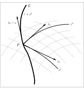
3.1 The Fermi normal coordinate system constructed along a geodesicG. . . 33
3.2 Parabolic orbits with different orbital angular momentum. . . 39
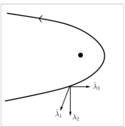
3.3 The spatial vectors of the rotated Fermi normal coordinate frame. . . 43
3.4 Acceleration terms in the metric of combined self- and tidal gravity fields. . . 51
4.1 Density profiles for 1D tests: Sod shock tube and two interacting blast waves. . . 69
4.2 2D density profile for Mach 3 wind tunnel with a step. . . 70
4.3 2D density profile for the double Mach reflection of a strong shock test. . . 70
4.4 Test density and analytical potential for Poisson solver. . . 80
4.5 Relative error between the analytical and computed gravitational potential. . . 81
4.6 Relative error in the x-derivative of the gravitational potential. . . 82
4.7 L2 error between the analytical and computed solution. . . 83
5.1 Trajectories of the FNC frame for two mass ratios in the black hole frame. . . 88
5.2 Stellar equilibrium model. . . 90
5.3 Weak tidal encounters. . . 92
5.4 Deflection of the center of mass off of the origin of the FNC. . . 94
5.5 Conservation of total angular momentum for Newtonian simulations. . . 95
5.6 Asymmetrical star with octupole tidal term. . . 97
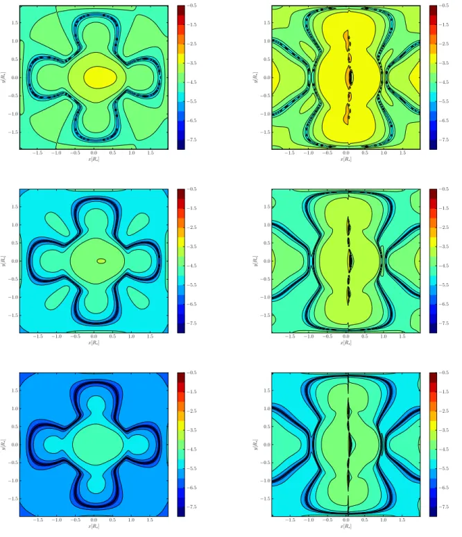
5.7 A snapshot of anη= 3 encounter in the black hole and FNC frame. . . 98
5.8 Partial and complete disruptions. . . 99
5.9 Density contours of anη= 3 encounter and mass ratioµ= 3.77×10⁻⁵. . . 100
5.10 Density contours of an η= 1 encounter and mass ratioµ= 3.77×10⁻⁵. . . 101
5.11 Vorticity contours of anη= 3 encounter and mass ratio µ= 3.77×10⁻⁵. . . 102
5.12 Vorticity contours of anη= 1 encounter and mass ratio µ= 3.77×10⁻⁵. . . 103
5.13 Comparison between full simulations and linear theory. . . 105
List of Tables
2.1 Properties given for different polytropes. . . 13
2.2 Polynomial coefficients for fit of dimensionless functionTl(η) forl= 2,3. . . 26
4.1 Second-order convergence of Poisson solver. . . 83
5.1 Properties of the star in CGS units . . . 87
5.2 Properties of the star in black hole mass units for different mass ratios . . . 87
5.3 Parameters for different types of encounters. . . 89
5.4 Wall clock time for simulating stellar equililbrium andη= 1−6 encounters. . . 93
5.5 Mass/energy outflow forη= 1−4 encounters. . . 97
5.6 Deposited energy ∆Etot onto the star for relativistic encounters. . . 104
5.7 Average energy and angular momentum deposited onto the star. . . 104
5.8 Dimensionless functionT2 from linear theory and simulations. . . 107
5.9 Energy excess due to radial oscillations and shock heating. . . 110
List of Abbreviations and Symbols
α, β, γ, . . . Schwarzschild coordinates indices running from 0 to 3
i, j, k, . . . Spatial coordinates indices running from 1 to 3
(a),(b),(c), . . . Schwarzschild standard tetrad coordinates
a, b, c, . . . Fermi normal coordinates
M∗ Mass of the star
R∗ Radius of the star
M Mass of the black hole
Rp Periastron distance from black hole
µ Mass ratioM∗/M
η Disruption parameter
ν Radius of the star to periastron distance ratioR∗/Rp
ηµν Minkowski metric
gµ0ν0 Schwarzschild coordinate metric
gab Fermi normal coordinate metric
Rµ0α0ν0β0 Riemann tensor in Schwarzschild coordinates
R(a)(b)(c)(d) Riemann tensor in Schwarzschild standard tetrad
Rabcd Riemann tensor in Fermi normal coordinates
Γα0
β0γ0 Connection coefficients in Schwarzschild coordinates
Chapter 1
Introduction
Lurking in most large galaxies are supermassive black holes. They reside in active and dormant
galaxies and their presence is revealed only through the interaction with their surroundings. The
best diagnostic for the presence of a black hole in a nonactive galaxy would be the tidal disruption
of stars [1, 2]. There are many observable signatures associated with this process. When a star
disrupts near a black hole, some of the debris is ejected from the system and the rest that is bound
eventually accretes onto the black hole. The fate of the debris is dependent on the type of star and
the mass and spin of the black hole. If the star is known, then a study of its tidal disruption will
provide an independent means of measuring the mass of the black hole from theM−σrelation, the
empirical correlation between the stellar velocity dispersionσof a galaxy bulge and the black hole
mass M at the center. From dynamical models of main-sequence stars, it is predicted that tidal
disruptions will occur once every 103-105 years for a non-spinning black hole of mass M
.108M
[3, 4]. A more massive black hole would result in a capture orbit instead of tidal disruption. For
maximally spinning black holes, the upper limit on the mass of the black hole may be increased
[5]. This suggests that solar-type star tidal disruption rates are dependent on black hole spin for
M ≥ 108M
. In this thesis, we are concerned with the tidal disruption of white dwarfs through
close encounters with a massive black hole.
By simulating the tidal disruption mechanism with a computer, we are able to provide theoretical
models to match observation of tidal disruption candidates. A flare of optical, UV, and X-ray
emission will occur promptly upon disruption and as captured gas streams back to the black hole after
one final orbit [1]. X-ray observatories Chandra and XMM-Newton observed the first tidal disruption
event candidates [2, 6]. Since then, obervations made in the optical, ultraviolet, and X-ray reveal
many more available for study [7, 8, 9, 10, 11, 12]. Recently, the unusual detection of long duration
γ-ray bursts for Swift J164449.3+573451 suggest that more tidal disruption candidates associated
with jet production are possible [13, 14, 15]. It is also of interest to use simulations to explain other
possible observational signatures such as the supernova-like remnant structures associated with the
ejection of debris [16, 17], the electromagnetic signal coupled with a gravitational wave event [18], and
The importance of including relativistic tidal effects in a computer simulation may be highlighted
by the recent unusual observations of Swift J1644+57. The Swift satellite detected a long duration
γ-ray burst and intense X-ray flares for several days followed by flares with significant decay [14]. A
precurser X-ray flare was also associated with these events. Typical GRBs reach similar luminosity,
but generally fall-off more rapidly. The detected X-ray luminosity ranged from 1045
−4×1048 erg
s−1, which suggests the release of gravitational energy by accretion of matter onto a black hole.
From the X-ray variability time-scale of the object,δtobs∼100 s, Burrows et al. [14] set the limit
on the black hole mass to be 106−2×10⁷M
. The presence of a radio transient also suggests a jet
hitting surrounding gas. The properties of this event are different from the standard tidal disruption
events and AGN jets. Bloom et al. [13] note that the two peaks in the broadband spectral energy
distribution represent synchrotron and inverse Compton processes, similar to what is expected for
blazars [13]. They propose that Swift J1644+57 is a small-scale blazar fed by the disruption of a
solar-type star by a 106
−107M
black hole. Krolik and Piran propose a different scenerio –a white
dwarf is disrupted by a.105M
intermediate mass black hole upon several successive encounters
[22]. A white dwarf has a greater density than a solar-type star and its presence may account for
the short timescales in the event. The series of flares are perhaps explained by the return of gas that
is stripped off of the white dwarf as it makes several encounters before disruption. Krolik and Piran
state that if this scenerio is correct then this event is the first indication of a black hole of mass
104
−105M
. In this thesis, we show that modeling the disruption between a star and a black hole
with mass smaller than 106M
requires the inclusion of relativistic terms in the tidal interaction.
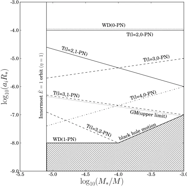
There are several interesting aspects of white dwarf – intermediate mass black hole encounters.
For mass ratios∼10−6and smaller, the Roche tidal radius is smaller than the Schwarzschild radius
and the white dwarf will be on a capture orbit. Therefore, in studying the tidal interaction, the
lower limit in mass ratio is∼10−6. For non-disruptive encounters, the normal modes of the white
dwarf can be excited non-resonantly and several successive encounters may lead to additional mode
excitation and heating. In the regime where gravitational radiation is the dominant mechanism for
the evolution of the orbit, resonant passages may excite modes [23, 20]. Significant energy transfer
may lead to an increase in temperature such that a thermonuclear runaway produces a Type Ia
supernova.
Several theoretical treatments to the problem of uncovering the cause of extremely luminous
sources at the centers of galaxies indicate that the debris from a tidally disrupted star is the culprit.
the change in the gravitational potential across the star [24, 1]. However, the nature of this problem
suggests that a full three-dimensional hydrodynamic treatment is necessary to determine the fate
of the disrupted star. Semi-analytic studies of the tidal interaction between close binaries provide
important details on the energy transfer during this process [25, 26, 27, 28]. Several numerical
methods have been used to model the disrupted star as it passes by the black hole on a parabolic
orbit. Several studies have implemented the affine model and results indicate that for orbits with
periastron much smaller the Roche tidal radius, the star will undergo severe compression and
“pan-cake” upon disruption [29]. Such encounters are interesting because of the possibility of triggering a
thermonuclear explosion. However, the main limitation of the affine model is that the star can only
be approximated as an ellipsoid. Using smooth particle hydrodynamics for tidal disruption adds
flexibility to solving the problem in that no approximations to the shape of the star are needed and
the full process is treated in a gridless manner [30]. This method is particularly useful in modeling
the fall-back of debris after a first encounter. Many works use Newtonian and relativistic versions
of the method [31, 32, 33, 34, 18, 35, 21]. The results of SPH methods are questionable because
of the production of spurious entropy in adding artificial viscosity to treat shock waves [36]. There
are a few comparisons of the SPH pancake mechanism simulations with one-dimensional finite
dif-ference methods (focusing on the compression orthogonal to the orbital plane) [18, 37]. Studies
using three-dimensional simulations with high-resolution shock-capturing techniques model the
dis-ruption in a coordinate system centered on the star. Newtonian hydrodynamics and self-gravity
is assumed for the star and a Newtonian quadrupole tide is used [38, 39, 40, 41]. A few studies
have implemented the effects of the black hole space-time [42, 43] and it is of interest to follow-up
these studies with higher resolution and a higher-order relativistic treatment to the black hole tidal
interaction. Recently, general relativistic hydrodynamic methods with adaptive mesh refinement
[44] and additionally with magnetohydrodynamics [45] have been applied to the disruption problem.
These methods are well-suited to modeling the accretion flare.
The purpose of this work is to study the disruption phase of the encounter, focusing on energy and
angular momentum deposition. We would like to be able to use these results as initial conditions in
subsequent computations of the fate of the post-disruption debris. In this thesis, we are interested in
the tidal disruption of white dwarfs by intermediate mass Schwarzschild black holes. In Chapter 2, we
begin by presenting the physics of tidal disruption in the Newtonian limit. We list the different phases
the star undergoes as it makes a close passage by the black hole. We introduce the linear theory of
dwarf and the black hole is presented. We introduce the coordinate system for our calculations, the
Fermi normal coordinates (FNC). We use Newtonian hydrodynamics and self-gravity for the star
and set a cut-off in the combined self-gravity and tidal gravity metric expansion at stellar 1-PN.
This restricts the number of terms we may use for our calculation of the tidal acceleration. Using
a post-Newtonian formalism, we justify our use of retained terms in the expansion. In Chapter 4,
we present the numerical method for simulating tidal disruption. We use the piecewise parabolic
method with Lagrangian remap (PPMLR) for the hydrodynamics solver. We use a pseudo-spectral
method to solve Poisson’s equation. We calculate the relativistic tidal acceleration using a routine
to update the location of the FNC frame along the geodesic using the hydrodynamic time as the
proper time. Finally, we give the results of our numerical method in Chapter 5. We consider
encounters at the threshold of disruption and weaker. We choose intermediate mass black holes
to be M ∼ 103M
,104M,105M. We first present a validation of the numerical method using a stellar equilibrium model. For our simulations with the tidal interaction, we use the relativistic
quadrupole and octupole terms. We note that the inclusion of the octupole term drives the center
of mass of the star off of the origin of the FNC frame. We compare the results for non-disruptive
encounters with the predictions from the linear theory. We give the amount of energy and
spin-angular momentum deposited onto the star and note a difference in the energy between Newtonian
Chapter 2
Physics of Tidal Disruption From the Newtonian Viewpoint
In this chapter we consider the tidal disruption of a star by a black hole in the Newtonian limit.
We begin by introducing general assumptions about the process and introduce the dimensionless
disruption parameterη, which characterizes the types of encounters in terms of the mass of the star,
the large central mass (black hole), the radius of the star, and the distance of closest approach.
Then, we consider physical effects that may occur when a star passes too close to a massive black
hole. For the most part the star is assumed to be a polytrope, which allows its envelope structure to
be described by a single parametern and serves as an approximation for a variety of objects (e.g.,
solar-type stars, white dwarfs, red giants, and neutron stars). In the second section, we discuss the
assumption of a polytropic equation of state and review solutions of the resulting equations of stellar
equilibrium. In the third section, we consider the consequences of a polytropic star in a Newtonian
tidal field. We find that the octupole tidal field causes the center of mass of an extended object
like a star to accelerate relative to the trajectory of a point mass. We discuss torques on the fluid
configuration. In the fourth section, we consider weak encounters where the star does not disrupt,
but may become (linearly) distorted. In this limit, we apply the linear theory of tidal interactions
and consider the amount of predicted total energy and (spin) angular momentum deposited onto
the star during the encounter. In the final section, we discuss disruptive encounters and the nature
of the resulting debris.
2.1 Overview of the process of tidal disruption
In the following, we describe how a star disrupts during an encounter with a heavy point mass
(black hole). In this chapter, we will refer to the central mass as a “black hole,” even though
we consider only Newtonian physics. We assume that far away from the black hole the star is in
spherical hydrostatic equilibrium, such that only the pressure forces and self-gravity of the gas are
in balance. If we consider encounters at the threshold of disruption, then roughly we can say that
at periastron the differential tidal acceleration across the star is comparable to or larger than its
of the star is less than or equal to the stellar pulsational timescale. Given these assumptions, an
encounter may be described by a dimensionless parameterη, the disruption parameter, such that
η= R
3
p M
M∗
R3 ∗
!1/2
, (2.1.1)
whereM∗,R∗, M, and Rp are the mass of the star, radius of the star, mass of the black hole, and
radius of periastron, respectively [26]. Tidal disruption occurs for η .1. Forη >1, the star does
not disrupt completely, though it may be partially stripped. We may define the tidal radius for
η = 1 where RT =R∗(M/M∗)1/3. We may also characterize these encounters with a penetration
factorβ=RT/Rp=η−2/3[19].
A fraction of gas from a star that has been disrupted or partially disrupted will return to
perias-tron after a last orbit and then presumably settle into an accretion disk about the black hole. The
nature of this gaseous debris depends on the stellar structure of the star and on the detailed
hydro-dynamic forces and residual self-gravity as the debris expands. After disruption, nearly Keplerian
motion will cause the gas to spread within the orbital plane and compressional bounce and envelope
shocks cause some gas to rise out of the orbital plane. Escaping gas cools and loses all significant
self-gravity, effectively freezing into a distribution of Keplerian orbits. Eventually hydrodynamic
forces become important again as inclined orbits intersect near apastron and as the stream returns
to periastron. For very close encounters, gas from the star may accrete onto the black hole
imme-diately. The tidal disruption process may described in phases: disruption (with possible prompt
accretion), sheared motion of debris, accretion upon return to pericenter, and possible repetitions of
debris orbits and accretion. The focus of this thesis is on the disruption phase, although the results
of the analysis are important for modeling the rest of the process.
2.2 Polytropes
In this section, we discuss the assumption that the star can be modeled effectively as a
poly-trope. Using thermodynamic considerations, we derive expressions to quantify the thermodynamic
description of the star. This is important later for the computational diagnostics of the simulations.
We show how to obtain density and pressure profiles of a star in terms of its polytropic index n
2.2.1 Thermodynamic considerations
Consider a system in terms of pressure p, volumeV, internal energyU, heat fluxQ, entropyS,
and temperatureT. Assume that it is hydrostatic, in equilibrium, and undergoes processes that are
reversible and adiabatic. Then, the heat flux is quasi-static and the entropy is constant [46, 47].
The first and second laws of thermodynamics are given by
dU =d¯Q−pdV, d¯Q=TdS= 0. (2.2.1)
For a perfect (ideal) gas, the equation of state is given by
pV =RT, U =U(T), (2.2.2)
with gas constant R = 8.314×10⁷ erg/deg mol and one assumes that the internal energy is a
function of temperature only. The heat capacity at constant volume is Cv = (∂U/∂T)v =dU/dT
and at constant pressure is Cp = (d¯Q/dT)p = Cv +R. Define the ratio of specific heats to be
γ =Cp/Cv = 1 +R/Cv. For monoatomic gases, γ = 5/3, and for diatomic gases, γ = 7/5. The
internal energy may be written asU =CvT =RT/(γ−1). Then, we can rewrite the equation of
state for an ideal gas as
pV =RT = (γ−1)U, p= (γ−1)ρε, (2.2.3)
in terms of the internal energyU or the specific internal energyε =U/M, where M is the molar
mass andρis the density.
Substituting the ideal gas equation of state into the combination of the first and second laws
in terms of specific quantities (heat per molar mass q =Q/M, specific volume τ =V /M, specific
entropys=S/M), we obtain
d¯q= 0 =dε+pdτ =τ dP+γ p
ρ2dρ or dp=γ
p
ρdρ (2.2.4)
and find that
∂p
∂ρ
s
=γp
ρ. (2.2.5)
small changes in the density and pressure and flow velocities smaller than the sound speed, then we
may derive an acoustic equation describing the propagation of sound waves using the conservation
of mass and momentum equation. Consider the small changes in the density and pressure to be
written asρ=ρ0+ ∆ρandp=p0+ ∆p. Then, the linearized conservation of mass equation may
be written as
∂ρ
∂t =−ρ
∂v
∂x −→
∂
∂t(∆ρ) =−ρ0 ∂v
∂x. (2.2.6)
The linearized conservation of momentum equation may be written as
ρ∂v
∂t =−
∂p
∂x =−
∂p
∂ρ
s
∂ρ
∂x
−→ρ0
∂v
∂t =−
∂p
∂ρ
s ∂
∂x(∆ρ) =−c
2 ∂
∂x(∆ρ), (2.2.7)
where we assume isentropic particle motion in the sound wave, ∆p = (∂p/∂ρ)s∆ρ, and c2 =
(∂p/∂ρ)s. Taking the partial time derivative of (2.2.6),
∂2
∂t2(∆ρ) =−ρ0
∂2v
∂t∂x, (2.2.8)
taking the partial time derivative of (2.2.7),
ρ0
∂2
∂x∂tv=−c
2∂2ρ
∂x2, (2.2.9)
and combining the two results we obtain a wave equation,
∂2
∂t2 −c 2 ∂2
∂x2
∆ρ= 0. (2.2.10)
The solutions are
∆ρ= ∆ρ(x±ct), (2.2.11)
where the disturbance propagates in the±xdirection with speedc of sound,
c2=
∂p
∂ρ
s
= γp
ρ =γRT. (2.2.12)
Re-writingdp= (γp/ρ)dρas [∂(lnp)/∂(lnρ)]s=γand integrating, and takingγandsconstant, we
obtain the polytropic equation of state,
for some κthat is a function of the specific entropy, s, which must be at least constant (adiabatic)
along stream lines in the fluid. For an isentropic gas (s= constant everywhere), we havep=κργ,
with a universal constantκ.
2.2.2 Completely degenerate, ideal Fermi gas equation of state
In this thesis we will be primarily interested in examining tidal encounters of white dwarfs.
For an isolated white dwarf at T = 0, it is degeneracy pressure that supports the star against
gravitational collapse. Assume the pressure is just due to electrons which may be described by a
cold, degenerate equation of state [47]. We define the Fermi momentum of the electron in terms of
its Fermi energyEF, the speed of lightc, and the mass of the electronmeasEF = (pF2c2+m2ec4)1/2.
We further define a dimensionless Fermi momentum as x=pf/(mec). The pressure of the gas is
given by [47]
pe =
mec2 λ3
e
φ(x) = 1.42180×1025φ(x) dyne cm−2,
φ(x) = 8π12
n
x(1 +x2)1/2(2x2/3
−1) + lnhx+ (1 +x2)1/2io, (2.2.14)
and the total energy density is given by
εe =
mec2 λ3
e χ(x),
χ(x) = 1
8π n
x(1 +x2)1/2(1 + 2x2)
−lnhx+ 1 +x21/2io
, (2.2.15)
where λe =~/(mec) is the Compton wavelength of the electron. Consider the non-relativistic and
relativistic limits of the equation of state in terms of the dimensionless Fermi momentum. For
non-relativistic electrons,x1, we have that
φ(x) → 151π2 x
5
−145x 7+ 5
24x 9
· · · ,
χ(x) → 1
3π2 x
3+ 3 10x
5
− 3
56x 7
· · ·
. (2.2.16)
For relativistic electrons,x1, we have that
φ(x) → 121π2 x
4
−x2+32ln 2x· · · ,
χ(x) → 1
4π2 x
4+x2
−1
2ln 2x· · ·
For the two limiting cases, the equation of state has a polytropic form, p = κργ, with (1)
non-relativistic electrons: ρ106g cm−3,x
1,φ(x)→x5/15π2,
κ= 3
2/3π4/3
5
~2 mem5
/3
u µ5
/3
e
=1.0036×10
13
µ5e/3
, γ=5
3, (2.2.18)
and (2) extremely relativistic electrons: ρ106g cm−3,x1,φ(x)→x4/12π2,
κ= 3
1/3π2/3
4
~c m4u/3µ4e/3
= 1.2435×10
15
µ4e/3
, γ= 43, (2.2.19)
where the numerical values are in cgs units and for atomic mass unitmu = 1.66057×10⁻²⁴g and
mean molecular weight per electron µe. Thus, in the limit of extreme non-relativistic and
ultra-relativistic electrons, the ideal Fermi gas equation of state reduces to a polytropic form.
2.2.3 Stellar equilibrium
Consider the equations of hydrostatic equilibrium for a spherically symmetric, non-relativistic
star [47, 46] of massM∗and radiusR∗. The mass interior to a radiusris given by
m(r) =
Z r
0
ρ4πr2dr, dm(r)
dr = 4πr
2ρ. (2.2.20)
Consider a fluid element betweenrandr+drwith an areadAperpendicular to the radial direction.
The gravitational force exerted on the elementdmdue to the mass interior toris equal to the net
outward pressure force ondm. Then, the equilibrium condition is
dp
dr =−
Gm(r)ρ
r2 . (2.2.21)
Consider the following quantities to obtain a virial theorem for the star. The gravitational potential
energy is given by
Ω = −
Z M
0
Gm(r)dm(r)
r =
Z R
0
dp dr4πr
3dr=
−3
Z R
0
p4πr2dr, (2.2.22)
where the pressure pat the surface of the star is zero. The internal energy isU =RR
0 ρ4πr 2dr=
RR
0 [p/(γ−1)]4πr
2dr, using the ideal gas equation of state. It follows that the relationship between
hydrostatic equilibrium is given by
Ω =−3(γ−1)U. (2.2.23)
Consider the thermal kinetic energy of this gaseous configuration. For a fluid element, there aredN
number of molecules and the kinetic energy for each molecule is 3kT/2. The total contribution for
the fluid element is thendET = 3kTdN/2 = 3(γ−1)cVTdm/2, in terms of specific heat cv. The
internal energy of the fluid element is given bydU =cVTdm. Then, for the whole configuration,
the thermal kinetic energy is given byET = 32(γ−1)U. In accordance with the virial theorem, it
follows thatET =−12Ω.
Equilibrium configurations characterized by a polytropic equation of state are referred to as
polytropes. Substituting the adiabatic (polytropic) equation of state into the expression for Ω
(2.2.22),
Ω =−3(γ−1) 5γ−6
GM2
∗
R∗ . (2.2.24)
The total energy of the polytrope is then
Etot=U+ Ω =−
3γ−4 5γ−6
GM∗2
R∗ . (2.2.25)
We next show how to obtain the dimensionless envelope structure of the polytrope, characterized
by the polytropic index n, using the Lane-Emden equation [46]. By combining the hydrostatic
equilibrium conditions, (2.2.20) and (2.2.21), we obtain the fundamental equation
1 r2
d dr
r2
ρ dP
dr
=−4πGρ. (2.2.26)
Define the polytropic indexnbyγ≡1 + 1/n. Consider the dimensionless Lane-Emden variablesξ
andθ(ξ) such that the radius of the star is
r=aξ, a=
(n+ 1)κ
4πG ρ
1/n−1
c
1/2
, (2.2.27)
where constant κ is defined by the equation of state p = κργ. Consider another dimensionless
variable and are given by
ρ(ξ) =ρcθ(ξ)n, p(ξ) =pcθ(ξ)n+1, (2.2.28)
whereρc andpc are the central values. We re-cast the fundamental equation (2.2.26) in terms of ξ
andθand obtain the Lane-Emden equation of index n,
1 ξ2
d dξ
ξ2dθ
dξ
=−θn. (2.2.29)
The boundary conditions at the origin are
θ
ξ=0= 1,
dθ dξ
ξ=0= 0. (2.2.30)
To get the density and pressure profiles, we must solve the Lane-Emden equation. Except for a few
specialn, this is done numerically. For n < 5, the solution decreases monotonically with the first
zeroθ(ξ1) = 0 corresponding to the surface of the star,
R∗=aξ1=
(n+ 1)κ 4πG ρ
1/n−1
c
ξ1. (2.2.31)
The central density and pressure are
ρc=−
ξ
3 1 dθn/dξ
ξ=ξ1
¯
ρ, pc=Wn
GM2
∗
R4 ∗
, (2.2.32)
where ¯ρ=M∗/(4πR3∗/3) andWn= [4π(n+ 1)[(dθn/dξ)ξ=ξ1]
2]−1. The total mass at a distanceξis
M∗(ξ) =−4πa3ρcξ2dθ/dξand for the entire star,
M∗ =−4π
(n+ 1)κ 4πG
3/2
ρ(3−n)/2n c
ξ2dθn
dξ
ξ=ξ1
. (2.2.33)
We eliminateρcfrom this equation using (2.2.31) to obtain themass-radius relationfor a polytrope,
GM∗(n−1)/nR∗(3−n)/n= (n+ 1)κ (4π)1/n
−ξ(n+1)/(n−1)dθn dξ
(n−1)/n
ξ=ξ1
Rewriting, the constantκin terms ofM∗ andR∗ is given by
κ=NnGM(
n−1)/n
∗ R(3∗−n)/n, Nn =
1
n+ 1
4π
0ωnn−1
1/n
, (2.2.35)
where 0ωn=−ξ(
n+1)/(n−1)
1 (dθn/dξ)ξ=ξ1.
Re-writing the fundamental equation (2.2.26) in terms of the self-gravitational potential Φ where
dp/dr=ρ(dΦ/dr), we have Poisson’s equation,
1 r2
d dr
r2dΦ
dr
=∇2Φ = 4πGρ. (2.2.36)
We may write the solution for inside and outside the star as
Φ(ξ) =
−4πGa2ρ
cθ(ξ)−GMR∗∗, r < R∗,
−GM∗
r , r≥R∗.
(2.2.37)
In Table 2.1, the first zero of the Lane-Emden equation and the relevant quantities for calculating
the central density and pressure are given for n=1.5, 2, and 3 polytropes [46, 49, 50].
n ξ1 (dθn/dξ)ξ=ξ1 −
hξ
3 1
dθn/dξ
i
ξ=ξ1
Remark
1.5 3.6537534 2.033013E-1 5.990705 (non-relativistic white dwarf) 2.0 4.35287460 1.272487E-1 1.140254E1
3.0 6.89684862 4.242976E-2 5.148248E1 (extreme relativistic white dwarf)
Table 2.1: Properties given for different polytropes. We give the first zero of the Lane-Emden equation,ξ1, and dθn/dξandξ(dθn/dξ)−1/3 evaluated atξ1.
2.3 Newtonian star in a Newtonian tidal field
In the following, the tidal interaction between the black hole and a polytropic star is presented
within the Newtonian formulation. The mass moments and other integrals characterizing the fluid
star are introduced [51, 29]. We show the effects of tidal heating and tidal spin-up of the star. We
derive the deviation between the equation of motion for the center of mass of the star and the origin
2.3.1 Momentum equation in a coordinate system following the star
Assume that the star is a Newtonian fluid. Consider an inertial coordinate system (Xk, T) with
origin fixed on the black hole (assuming the black hole is so massive its motion can be neglected).
The velocity of the material moving in the gravitational field of the black hole will be taken to be
Vk(T). The density and pressure areρ(Xk, T) andp(Xk, T). The convective derivative taken along
streamlines (Stokes time derivative) is given by
d
dT =
∂
∂T +Vk
∂
∂Xk
. (2.3.1)
The continuity equation for the fluid in the black hole frame is written as
dρ
dT +ρ
∂Vk ∂Xk = ∂ρ ∂T + ∂ ∂Xk
(ρVk) = 0 (2.3.2)
and the momentum equation is written as
ρdVk
dT =ρ
∂Vk
∂T +ρVl
∂Vk ∂Xl
=−∂X∂p
k −
ρ∂Φ
∗
∂Xk
+ρgtk, (2.3.3)
where Φ∗is the star’s self-gravitational potential andgt
k is the external black hole tidal acceleration
field.
LetXk(0)(T) andVk(0)(T) =dXk(0)/dT denote the position and velocity of the origin of a
coordi-nate system following the star (in a way to be described precisely below). Define
xk =Xk−X
(0)
k (T) vk =Vk−V
(0)
k (T), (2.3.4)
as positions and velocities relative to the origin of the moving system. We rewrite the continuity
and momentum equations in this frame (xk, t) by considering the following change of variables. Let
f ={xk, t} andg={Xk, T}. The Jacobian matrix is
J = ∂f1 ∂g1 ∂f2 ∂g1 ∂f1 ∂g2 ∂f2 ∂g2 = ∂xk ∂Xk ∂t ∂Xk ∂xk ∂T ∂t ∂T = 1 0
−Vk(0) 1
. (2.3.5)
Then, the change of variables is the following,
∂ ∂Xk = ∂ ∂xk , ∂ ∂T = ∂
∂t−V
(0)
l ∂ ∂xl
The continuity equation in a coordinate frame following the star is then
∂ρ
∂t −V
(0) k ∂ρ ∂xk + ∂ ∂xk h
ρ(Vk(0)+vk) i
= ∂ρ
∂t +
∂ ∂xk
(ρvk) = 0, (2.3.7)
where ∂Vk(0)/∂xk = 0. This has the same form as the equation in the black hole frame. Similarly,
we apply the transformation to the momentum equation and get
ρ∂vk
∂t +ρvl
∂vk ∂xl
=ρdvk
dt =−
∂p
∂xk −
ρ∂Φ
∗
∂xk
+ρgtk−ρ dVk(0)
dt , (2.3.8)
where−ρdVk(0)/dtis the coordinate acceleration term.
2.3.2 Relevant moments and tensors defined
Consider the following theorem, for any quantity Q(xk, t),
d dt
Z
ρ Qd3x=
Z
ρdQ
dt d
3x. (2.3.9)
This may be proved by introducing Lagrangian coordinates,ξk, fixed to the fluid elements, where
xk =xk(ξl, t), dxk = ∂xk
∂ξl dξl+
∂xk
∂t dt, vk=
∂xk ∂ξl
˙ ξl+
∂xk
∂t . (2.3.10)
The transformation between different volume elements, connected by JacobianJisd3x=
|∂xk/∂ξl| ≡
Jd3ξ. Then,
d dt ∂xk ∂ξl
= ∂xk ∂ξm∂ξl
˙
ξm+
∂xk ∂t∂ξl = ∂ ∂ξl ∂xk ∂ξm ˙
ξm+
∂xk ∂t
=∂vk ∂ξl
, (2.3.11)
where in the new coordinate systemξmand ˙ξmare independent, so that∂ξ˙m/∂ξk= 0. We write
d dt
Z
ρ Qd3x = d
dt Z
ρ QJd3ξ=Z Qd
dt(ρJ)d
3ξ+Z dQ
dtρJd
3ξ (2.3.12)
=
Z Q
dρ
dtJ+ρ
dJ dt
d3ξ+
Z dQ dtρJd 3ξ = Z Q dρ
dt +ρ
d dtlnJ
Jd3ξ+
Z dQ
dtρJd
3ξ=Z dQ
dtρJd
3ξ,
where we have that
dρ
dt =−ρ
∂vk ∂xk
, and d
dtlnJ =
∂ξl ∂xk d dt ∂x k ∂ξl
= ∂ξl ∂xk
∂vk ∂ξl
= ∂vk ∂xk
Thezeroth moment (Q= 1) is defined as
M∗≡
Z
V
ρd3x, (2.3.14)
over a volumeV. Define thefirst mass moment and derivatives as
Dk ≡
Z
V
ρxkd3x, D˙k=
Z
V
ρvkd3x, D¨k =
Z
V
ρdvx
dt d
3x. (2.3.15)
Themoment of inertia tensor, or second mass moment, and its derivative are defined as
Iij ≡ Z
V
ρxixjd3x, I˙ij=
Z
V
ρ(xivj+vixj)d3x. (2.3.16)
Themoment of inertiaI follows from taking the trace,
I≡Iii = Z
V
ρr2d3x. (2.3.17)
Likewise we can define a third moment, oroctupole moment tensor, as
Iijk = Z
ρxixjxkd3x. (2.3.18)
The fluid configuration may have angular momentum, which is described by the tensor,
Jij ≡ 12 Z
V
ρ(xivj−vixj)d3x. (2.3.19)
We see that
Z
V
ρxivjd3x= 12I˙ij+Jij,
Z
V
ρvixjd3x= 21I˙ij−Jij, (2.3.20)
whereIij =Iji andJij=−Jji[51, 29]. Thekinetic energy tensor andkinetic energy are defined as
Tij≡ 12 Z
V
ρvivjd3x, T ≡Tii=12
Z
V
ρv2d3x. (2.3.21)
With all of this in hand, it is possible to make the following connection,
Z
V
Next, we consider the gravitational effects. Define theself-gravitational potential as
Φ∗(x)≡ −G Z
V
ρ(x0)d3x0
|x−x0| (2.3.23)
and theself-gravitational potential energy as
Ω≡1 2
Z
V
Φ∗ρd3x≡ −1 2G
Z
V
Z
V
ρ(x)ρ(x0)d3xd3x0
|x−x0| . (2.3.24)
This scalar quantity is a part of a more generalself-gravitational energy tensor, given by
Ωij≡ −12G
Z Z (x
i−x0i)(xj−x0j)
|x−x0|3 ρ(x)ρ(x
0)d3xd3x0. (2.3.25)
Then, we see that Ω = Ωii. Consider the spatial derivative of Φ∗,
∂iΦ∗=−G Z
V
xi−x0i |x−x0|3ρ(x0)d
3x0. (2.3.26)
Then, due to symmetry it is fairly easy to show that
− Z
xi(∂jΦ∗)ρd3x =−G
Z Z x
i(xj−x0j)
|x−x0| ρ(x)ρ(x
0)d3xd3x0
=−1 2G
Z Z (x
i−x0i)(xj−x0j)
|x−x0| ρ(x)ρ(x
0)d3xd3x0
= Ωij. (2.3.27)
From the symmetry of Ωij it follows that
Z
xi(∂jΦ∗)ρd3x= Z
xj(∂iΦ∗)ρd3x. (2.3.28)
Note that thegravitational self-force vanishes,
Z
(∂iΦ∗)ρd3x=G
Z x
i−x0i
|x−x0|3ρ(x)ρ(x0)d
3xd3x0= 0, (2.3.29)
as can be seen by the interchange ofxk ↔x0k. Then we have an important alternative expression
for the gravitational energy,
Ω =12
Z
Φ∗ρd3x=− Z
Thegravitational self-potential tensor is defined as
Φ∗ij≡ −G
Z (x
i−x0i)(xj−x0j)
|x−x0|3 ρ(x0)d
3x0, (2.3.31)
where
Ωij = 12 Z
Φ∗ijρd
3x. (2.3.32)
With some work, we can show that therate of change of gravitational energy is
˙ Ω =
Z
vi∂iΦ∗ρd3x. (2.3.33)
We now consider the various fluid energies. The pressure moments are given by
Π =
Z
V
pd3x, Πi=
Z
V
pxid3x, Πij =
Z
V
pxixjd3x. (2.3.34)
We can show that thechange in total internal energy is
˙
U =
Z
vk∂kpd3x. (2.3.35)
Consider the effects of an external gravitational field. Let the external force density be ft
i =
ρgt
i =−ρ∂iΦt. Then, we have thenet force on the fluid and themoment of force tensor,
Ft
i =
Z ft
id
3x=Z ρgt
id
3x, Ft
ij =
Z xifjtd
3x=Z x
igjtρd
3x. (2.3.36)
Therate at which work is done by the external forceis
˙
Wt=
Z
vifitd3x= Z
vigitρd3x. (2.3.37)
We have obtained the gravitational potentials and energies and energies associated with the fluid.
We will use these quantities in the following to calculate the rate of change of energy of the star
and will later include the work done by the external gravitational field and the acceleration of the
2.3.3 Equation of motion for the origin of the coordinate system following the star
Consider the momentum equation (2.3.8) in the moving frame. We can integrate the momentum
equation over a comoving volume,
Z
V
ρdvk
dt d
3x=
: 0 − Z V ∂p ∂xkd
3x − * 0 Z V
ρ∂Φ
∗
∂xkd
3x+Ft
k−M∗V˙k(0). (2.3.38)
Two of the terms vanish (as shown) because (1) the pressure at the surface of the fluid configuration
is assumed to vanish and (2) the gravitational self-force is zero, as we previously showed. Writing
in terms of the first moment, we find
Z
V
ρdvk
dt d
3x= d
dt Z
ρvkd3x= d2
dt2
Z
ρxkd3x= d2
dt2Dk, (2.3.39)
Thus we have a relationship between the acceleration of the coordinate system, ˙Vk(0), the net external
force,Ft
k, and the motion of the fluid configuration,
¨
Dk =Fkt−M∗V˙k(0). (2.3.40)
We are free to choose ˙Vk(0). We may enforce the initial condition Dk = 0 and ˙Dk = 0. If we take
the acceleration of the frame ˙Vk(0)to be equal to the external accelerationFt
k/M∗, then the center of
mass does not accelerate in the coordinate frame{xk} and the frame following the star{xk}is the
center-of-mass (CM) frame. Alternatively, we might take ˙Vk(0) to be that of a point mass (original
center of mass) moving in the external potential. The forces applied to the extended body can drive
apparent acceleration of the CM. In our calculations we choose this latter case in considering the
relativistic tidal field in Chapter 3.
2.3.4 Tensor virial theorem
Consider the first moment of the momentum equation in a frame following the star, (2.3.8),
Z
V
xiρ dvk
dt d
3x=
− Z
V
xi ∂p ∂xkd
3x
− Z
V
xiρ ∂Φ∗ ∂xkd
3x+Z V
xigtkρd
3x
− Z
V
ρxiV˙
(0)
k d
3x. (2.3.41)
Then, from previous definitions of moments and tensors, Subsection 2.3.2,
1
2I¨ik+ ˙Jik−2Tik= Πδik+ Ωik+Fikt −DiV˙
(0)
We may split this into antisymmetric and symmetric parts,
˙
Jik = 12(Fikt −F t
ki)−12
DiV˙k(0)−DkV˙i(0)
1
2I¨ik = 2Tik+ Πδik+ Ωik+12(Fik+Fki)−12(DiV˙
(0)
k +DkV˙
(0)
i ). (2.3.43)
In the center-of-mass frame (Di = 0) and without an external force (Fik = 0), the spin angular
momentum of the star is conserved ( ˙Jik= 0) and we have the following tensor virial theorem,
1
2I¨ik= 2Tik+ Πδik+ Ωik. (2.3.44)
2.3.5 Rate of change of energy of the star
We may contract the momentum equation in the frame following the star (2.3.8) with vk and
integrate
Z
ρvkv˙kd3x = − Z
vk∂kpd3x− Z
vk(∂kΦ∗)ρd3x+ Z
vkgtkρd
3x
− Z
vkV˙k(0)ρd3x
1 2
d dt
Z
ρvkvkd3x = −
dU
dt −
dΩ
dt + ˙W
t −D˙kV˙
(0)
k
˙
T+ ˙U+ ˙Ω = W˙ t
−D˙kV˙
(0)
k , (2.3.45)
and obtain the rate of change of energy of the fluid. The left hand side is the rate of change of total
energy of the fluid in the accelerated frame without external forces. The right hand side is the rate
at which work is done by the external gravitational field and a correction term if the accelerated
frame is not the center of mass frame. We obtain an expression for the work done by the tidal field,
˙
Wt, in the following. Let Φt(X
k, t) be the external potential from whichgkt is derived,
gt
k=−
∂
∂Xk
Φt= −∂x∂
k
Φt=
−∂kΦt. (2.3.46)
Then,
˙
Wt =
Z
ρvkgktd3x=− Z
vk(∂kΦt)ρd3x=−
Z dΦt
dt −
∂Φt ∂t
ρd3x
= −dtd Z
Φtρd3x+Z ∂Φt
∂t ρd
The external gravitational energy of the star is given by Θ =R
Φtρd3x. Then, using the
transfor-mation of the partial derivative of the inertial frame time,
˙
Wt =
−Θ +˙
Z ∂
∂T +V
(0)
k ∂k
Φt
ρd3x
= −Θ +˙ Ft
kV
(0)
k +
Z ∂Φt
∂T
ρd3x. (2.3.48)
With the equation of motion of the center of mass, (2.3.40), we have an expression for the work done
by the tidal field,
˙
Wt=−Θ˙ −1 2M∗
d dt
Vk(0)V
(0)
k
−D¨kV
(0)
k +
Z
∂Φt ∂T
ρd3x. (2.3.49)
Define the bulkkinetic energy of a star as seen in the inertial frame to be
T(0)= 12M∗Vk(0)V
(0)
k . (2.3.50)
The time dependence of the total energy is then
d
dt(T+U+ Ω) + d
dtΘ +
d
dtT(0)=− d dt
˙ Dkvk(0)
+
Z
∂Φt ∂T
ρd3x. (2.3.51)
If we choose the center-of-mass frame, then Dk = 0. If we further assume there is no intrinsic
variations in the external potential, e.g. ∂Φt/∂T = 0, then the total energy is conserved.
2.3.6 Tidal potential and tidal field
In the following, we will specify the form of the external force. In this section, we will assume
it derives from the potential of a heavy point mass and is time dependent. Expanding the tidal
potential Φtabout some trajectoryX(0)
k (t),
Φt = Φ(0)t −g
(0)
i xi+12C
(0)
ij xixj+16C
(0)
ijkxixjxk+241C
(0)
ijklxixjxkxl+· · ·,
gt
k = −∂kΦt=g(0)k −C
(0)
where [R2
(0)(t) =X (0)
k X
(0)
k ],
Φ(0)t = −
GM∗
R(0)
, g(0)k =−
GM∗Xk(0) R3
(0)
,
Cij(0) = ∂i∂jΦt (0)= GM∗ R5 (0)
δijR(0)2 −3X (0) i X (0) j ,
Cijk(0) = ∂i∂j∂kΦt (0)= GM∗ R7 (0)
15Xi(0)X
(0)
j X
(0)
k −3R
2 (0)X
(0)
j δik−3R2(0)Xk(0)δij−3R2(0)Xi(0)δjk
,
etc. Thenet force is then
Fk(0) = Z
ρgt
kd
3x=M
∗gk(0)−C
(0)
ki Di−12Ckij(0)Iij−16Ckijl(0)Iijl+· · ·. (2.3.53)
Thefirst moment of the force density is
Fij = Z
xigtjρd3x=Dig
(0)
j −C
(0)
jkIik−12C
(0)
jklIikl+· · ·. (2.3.54)
The rate of work done by the tidal field becomes
˙
Wt=
Z
ρvkgtkd
3x= ˙D
kgk(0)−Cki(0)
Z
ρvkxid3x−12Ckij(0) Z
ρvkxixjd3x+· · ·. (2.3.55)
Note that
Z
ρvkxid3x= 21I˙ik+Jik, (2.3.56)
from above, and that the productCki(0)Jikvanishes sinceCkiis symmetric andJikis antisymmetric.
DefineMijk≡ R
ρvixjxkd3x, whereMijk=Mikj. We see that
˙ Iijk =
Z
ρ(vixjxk+vjxixk+vkxixj)d3x=Mijk+Mjik+Mkij. (2.3.57)
and
Ckij(0)Mkij= 13
Ckij(0)+Cijk(0)+Cjik(0)Mkij= 13Ckij(0)I˙ijk. (2.3.58)
Then, the tidal gravitational work has the expansion,
˙ Wt= ˙D
kg (0) k − 1 2C (0)
ki I˙ik−16C
(0)
We can also obtain an expansion for the external gravitational energy of the star,
Θ =M∗Φ(0)t −Dig(0)i +12C (0)
ij Iij+16Cijk(0)Iijk+· · · . (2.3.60)
2.3.7 Center of mass frame vs. point-particle frame
We may rewrite the equation of motion for the origin of a coordinate system following the star
(2.3.40) and substitute the net force (2.3.53) to get
M∗X¨k+ ¨Dk =gk−Cki(X)Di−21Ckij(X)Iij−16Ckijl(X)Iijl+· · ·. (2.3.61)
For center of mass coordinates, we setDk and its derivatives to be zero. Then,
M∗X¨k(0)=−GM∗ Xk(0)
R3 −
1
2Ckij(X(0))Iij−16Ckijl(X(0))Iijl+· · · , D¨k= 0. (2.3.62)
If we would like to use CM coordinates, then equation (2.3.62) must be integrated in time.
Further-more, the motion of the origin is affected not only by the external point potential but also by the
octupole and higher-order tides.
If the coordinate system follows a point particle trajectory, then the origin is not guaranteed to
be coincident with the center of mass. Then the equation of motion for the origin is
M∗X¨k(p)=−GM∗ Xk(p)
R3
p
, (2.3.63)
and the mass moment evolves according to,
¨
Dk=−Cki(X(p))Di−12Ckij(X(p))Iij−16Ckijl(X(p))Iijl+· · ·. (2.3.64)
We see that the center of mass will follow a trajectory that accelerates away from the point-particle
trajectory,gk(X) =GM∗Xk/R3, because of the octupole tide and higher order corrections. Letζk
be the difference in position of the center of mass and the point particle trajectory,ζk ≡Xk−X(
p)
k .
Then, the deflection of the center of mass from the origin of the coordinate system following the star
is given by the following,
¨
ζk=−12Ckij(X)
1
M∗Iij(t)− 1
6Ckijl(X)
1
2.3.8 Change in orbital angular momentum due to the spin-up of star and acceleration of center of mass
We write the total angular momentum of the star in the black hole frame as
Jkl= Z
d3Xρ(X, t)(XkVl−XlVk). (2.3.66)
We substituteXk =xk+X
(0)
k (t) andVk =vk+V
(0)
k (t) to obtain an expression accounting for the
spin angular momentum and the position and velocity of the center of mass with respect to the
origin of the point-particle frame. We have that
Jkl =
Z
d3xρh(x+X(0))k(v+V(0))l−(x+X(0))k(v+V(0))l i
=
Z
d3xρ(xivj−vixj) + Z
d3xρ(xkVl(0)−xlVk(0))
− Z
d3xρ(v
kX
(0)
l −vlX
(0)
k ) +
Z
d3xρ(X(0)
k V
(0)
l −X
(0)
l V
(0)
k )
= Jkl+DkV
(0)
l −DlV
(0)
k −D˙kX
(0)
l + ˙DlX
(0)
k +M∗(X
(0)
k V
(0)
l −X
(0)
l V
(0)
k ),
where Jkl is the spin angular momentum in the point-particle frame (2.3.19) and Dl is the first
mass moment defined by (2.3.15). The time rate of change of the last term vanishes if we choose a
point-particle trajectory for the reference frame that does not change. The time rate of change of
total angular momentum is
˙
Jkl= ˙Jkl+ d dt
DkVl(0)−DlVk(0)−D˙kXl(0)+ ˙DlXk(0)
, (2.3.67)
where the first term corresponds to the change in spin angular momentum of the star and the rest
corresponds to the change in orbital angular momentum.
2.4 Non-disruptive encounters
2.4.1 Regime of weak tidal interactions
Consider encounters of a star with a black hole characterized by η >1. The tidal interaction
is weak and the star does not disrupt upon passing the black hole, but becomes distorted or and
excited into a set of pulsational modes. Gas may be tidally stripped off of the star. For
the excitation of the non-radial oscillations of the perturbed star [26, 52, 27, 38].
Under this formalism, we assume that the star is initially spherically symmetric, static, and in
hydrostatic equilibrium. The tidal interaction induces a slight perturbation from the initial state. We
write the perturbed variablef0 in terms of the initial statef and the pertubationδf asf0=f+δf
and obtain linearized versions of the equations of hydrodynamics and heat flow by neglecting all
powers above the first and products of the variations. We may express the perturbation variables
in terms of spherical harmonics and associate with each l, ma set of normal modes of oscillation,
representing a fundamental mode and overtones. Stars will pulsate in both pressure modes (p-modes)
and gravity modes (g-modes).
2.4.2 Energy and angular momentum deposited on the star
The amount of orbital energy deposited into oscillatory modes during a close periastron passage
depends upon two dimensionless parameters: the dimensionless envelope structure of the star, the
polytropic index n, and the dimensionless parameter characterizing the encounter, the disruption
parameterη [26]. We calculate the amount of energy removed from the orbit and deposited onto
the star as follows.
Consider a coordinate system centered on the star in the orbital plane. Letρbe the density of
the star,~vbe the fluid velocity, andU be defined asU(~r, t) =−Φt=GM/
|~r−R~(t)|, where R~(t) is
the relative orbit of the point mass,M. The rate at which energy is deposited onto the star is given
by
dE
dt = ˙W
t=
Z
d3xρ~v·∇~U =< ~v|∇~U > . (2.4.1)
Consider a linearized perturbation analysis on the effect of∇~U on the equilibrium star. Letρbe the
unperturbed stellar density. Express the fluid velocity in terms of a Lagrangian displacementξof the
fluid element from its unperturbed position as~v=∂ξ/∂t, where the Fourier transform ofξmay be
analyzed into normal modes. These normal modes satisfy a linear, self-adjoint eigenvalue equation
and may be written in terms of spherical harmonics. The amplitude of the tidal perturbation is of the
formUlm∼GM rl/R(t)l+1, in terms of spherical harmonic indiceslandm. The time dependence of
the perturbation inUlm is fixed by Keplerian motion and the disruption parameterη (2.1.1), which
relates the duration of periastron passage to the hydrodynamic timescale of the star. Thus, for a
into oscillations of spherical harmonic indexl is then
∆El=
GM2
∗
R∗
M
M∗
2R
∗
Rp
2l+2
Tl(η), (2.4.2)
whereTl(η) is a dimensionless function and may be explicitly calculated using the normal modes for
a given polytrope of indexn. The total energy is given by ∆E=P
l=2,3,...∆El. The dimensionless
functionTl(η) is calculated forn= 3 polytropes in Press and Teukolsky [26] and forn= 1.5,2,3 in
Lee and Ostriker (1986) [27]. It is shown that thel = 2 f-mode dominate the tidal energy transfer.
A quick method for obtaining the results from the latter was given by Portegies Zwart and Meinen
(1993) [53]. We obtainTl from the following polynomial,
logTl(η) =A+Bx+Cx2+Dx3+Ex4+Fx5, (2.4.3)
wherex= logη. Table 2.2 gives the polynomial coefficients for thel= 2 andl = 3 contribution to
(2.4.3) for a polytrope of indexn= 1.5.
n=1.5 l=2 l=3
A -0.397 -0.909
B 1.678 1.574
C 1.277 12.37
D -12.42 -57.40
E 9.446 80.10
F -5.550 -46.43
Table 2.2: Polynomial coefficients for fit of dimensionless functionTl(η) forl= 2,3. These are given
for ann= 1.5 polytrope.
Along with energy, the black hole deposits angular momentum onto the star. A star that is
initally at rest will “spin-up” as it passes by the black hole. From studies in comparing the affine
model with the linear theory, it is found that although energy is transferred into thel= 2,m=−2
f-mode, which should possess angular momentum and vorticity, the star bulk rotates just enough to
cancel out the vorticity [28]. It is shown that the star may be modeled as an irrotational ellipsoid.
Thus, for weak encounters, we may assume that the energy, ∆E, and angular momentum, ∆L,
deposited onto the star are related by
∆E' √|Ω|
15 ∆L p
I∗|Ω|, (2.4.4)
where I∗ = 13
R
energy of the star [28]. Despite the relativistic treatment of the tidal field in our calculations (Chapter
3), the special coordinate system that we use allows us to apply the Newtonian linear perturbation
theory in the limit of weak encounters.
2.5 Disruptive encounters
In this section, we describe the situation where the star disrupts and make some estimates for
the debris that is released during this type of encounter. We will see in this analysis a dependence
on various dimensionless parameters.
2.5.1 Spread of energies
Consider the following quantities associated with the Newtonian parabolic orbit of the star. The
velocity at periastron isvp = (2GM/Rp)1/2. The angular momentum islp =M∗(2GM rp)1/2. The
specific kinetic energy at periastron is p=GM/Rp. The gravitational potential of the black hole
at periastron is |Φp|=GM/Rp. As discussed in Rees (1988) [1] and Evans and Kochanek (1989)
[32], the tides will raise on the star and as the bulge attempts to stay aligned with the direction of
the black hole the star will be torqued. The maximal surface velocity is v∗ = (2GM∗/R∗)1/2. The
maximal spin angular momentum isl∗ =M∗(2GM∗R∗)1/2. The specific binding energy of the star
is∗=GM∗/R∗. The self-gravitational potential of the star at the stellar radius is|Φ∗|=GM∗/R∗.
We compare the quantities associated with the star and the orbit in terms of the mass ratio µ=
M∗/M, which we regard as small (µ1), and the disruption parameterη as
v∗
vp
=µ1/3η−1/3, l∗
lp
=µ2/3η1/3, ∗
p
=µ2/3η−2/3, Φ∗ Φp
= (µη)2/3. (2.5.1)
The disruption of the star reduces the specific orbital energy, p, by the specific binding energy,
∗. The variation in the specific energy of the released gas, ∆, depends on the change in the black
hole potential across the diameter of the star [1, 32, 54]. For a star at periastron, the gravitational
potential atRp+R∗ andRp−R∗ may be written as
±=−
GM
Rp±R∗ =−
GM Rp
1±RR∗ p
−1
=−GMR p
1∓RR∗ p
The spread of energies of the gas is then
∆= GM
Rp R∗
Rp
=pµ1/3=∗µ−1/3η2/3. (2.5.3)
Note thatp∆∗.
Since the variation in the specific energy of the released gas is much larger than the specific
binding energy, in the absence of hydrodynamic forces, we estimate that roughly 50% of the star
(located fromr=Rp tor=Rp+R∗) will become unbound during disruption while the other half,
fromr=Rp−R∗tor=Rp, will return to periastron after following a set of highly eccentric orbits.
The maximum velocity at infinity of the ejected debris may be given asvesc= (2∆)1/2.
2.5.2 Accretion rate
Once disruption occurs, the kinetic energy of the expanding debris is much larger than the
adi-abatically decreasing internal energy and diminishing self-gravitional energy. Thus, we can describe
the debris as locked into Keplerian trajectories and estimate a spread of energy of '2∆ with a
mass distribution ofdM/d'M∗/2∆[32]. The total energy of the most tightly bound gas can be
related to a semi-major axisamby ∆=−GM/(2am). Then,
am=−
GM 2∆ =GM
Rp
2GM
Rp R∗
= R
2
p
2R∗. (2.5.4)
The minimum (Keplerian) period before return to the hole is then
τm=
2πa3m/2 √
GM =
π √
2GM R2
p R∗
!3/2
. (2.5.5)
We may write
d
dτ =
d da
da
dτ =
1
3(2πGM) 2/3
τ−5/3. (2.5.6)
The estimated rate at which mass returns to the black hole after one post-disruption orbit is
dM∗
dτ =
dM∗
d d
dτ =
M∗
2
R
∗
Rp GM
Rp
1
3(2πGM) 2/3
τ−5/3= 13M∗ τm
τ
τm −5/3
. (2.5.7)
Newtonian simulations of debris motion after disruption appear to confirm this expected τ−5/3
dependence [32, 34, 35].