Mass Assembly of Stellar Systems and their Evolution with the SMA – 1.3 mm Subcompact Data Release
Ian W. Stephens,1 Michael M. Dunham,2, 1 Philip C. Myers,1 Riwaj Pokhrel,1, 3 Tyler L. Bourke,4 Eduard I. Vorobyov,5, 6 John J. Tobin,7, 8 Sarah I. Sadavoy,1 Jaime E. Pineda,9 Stella S. R. Offner,10 Katherine I. Lee,1 Lars E. Kristensen,11Jes K. Jørgensen,12 Alyssa A. Goodman,1 H´ector G. Arce,13 and
Mark Gurwell1
1Harvard-Smithsonian Center for Astrophysics, 60 Garden Street, Cambridge, MA, USA
2Department of Physics, State University of New York at Fredonia, 280 Central Ave, Fredonia, NY 14063, USA 3Department of Astronomy, University of Massachusetts, Amherst, MA 01003, USA
4SKA Organization, Jodrell Bank Observatory, Lower Withington, Macclesfield, Cheshire SK11 9DL, UK 5Research Institute of Physics, Southern Federal University, Stachki Ave. 194, Rostov-on-Don, 344090, Russia
6University of Vienna, Department of Astrophysics, Vienna, 1180, Austria
7Homer L. Dodge Department of Physics and Astronomy, University of Oklahoma, 440 W. Brooks Street, Norman, OK 73019, USA 8Leiden Observatory, Leiden University, P.O. Box 9513, 2300-RA Leiden, The Netherlands
9Max-Planck-Institut f¨ur extraterrestrische Physik, D-85748 Garching, Germany 10Department of Astronomy, The University of Texas at Austin, Austin, TX 78712, USA
11Centre for Star and Planet Formation, Niels Bohr Institute and Natural History Museum of Denmark, University of Copenhagen, Øster Voldgade 5-7, DK-1350 Copenhagen K, Denmark
12Niels Bohr Institute and Center for Star and Planet Formation, Copenhagen University, DK-1350 Copenhagen K., Denmark 13Department of Astronomy, Yale University, New Haven, CT 06520, USA
(Accepted to ApJS on June 17, 2018)
ABSTRACT
We present the Mass Assembly of Stellar Systems and their Evolution with the SMA (MASSES) survey, which uses the Submillimeter Array (SMA) interferometer to map the continuum and molecular lines for all 74 known Class 0/I protostellar systems in the Perseus molecular cloud. The primary goal of the survey is to observe an unbiased sample of young protostars in a single molecular cloud so that we can characterize the evolution of protostars. This paper releases the MASSES 1.3 mm data from the subcompact configuration (∼400 or ∼1000 au resolution), which is the SMA’s most compact array configuration. We release both uv visibility data and imaged data for the spectral lines CO(2–1),
13CO(2–1), C18O(2–1), and N
2D+(3–2), as well as for the 1.3 mm continuum. We identify the tracers
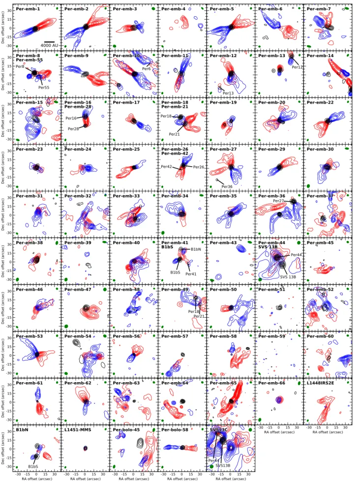
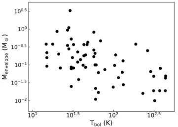
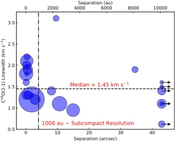
that are detected toward each source. We also show example images of continuum and CO(2–1) outflows, analyze C18O(2–1) spectra, and present data from the SVS 13 star-forming region. The calculated envelope masses from the continuum show a decreasing trend with bolometric temperature (a proxy for age). Typical C18O(2–1) linewidths are 1.45 km s−1, which is higher than the C18O
linewidths detected toward Perseus filaments and cores. We find that N2D+(3–2) is significantly
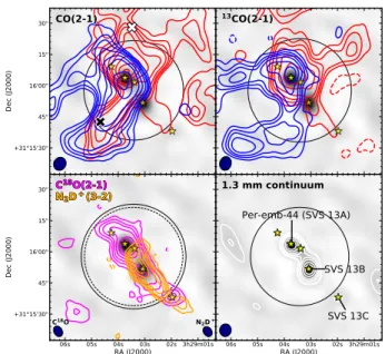
more likely to be detected toward younger protostars. We show that the protostars in SVS 13 are contained within filamentary structures as traced by C18O(2–1) and N
2D+(3–2). We also present the
locations of SVS 13A’s high velocity (absolute line-of-sight velocities>150 km s−1) red and blue outflow components. Data can be downloaded fromhttps://dataverse.harvard.edu/dataverse/MASSES.
Keywords: editorials, notices — miscellaneous — catalogs — surveys
1. INTRODUCTION
Stars are assembled in molecular clouds through the gravitational collapse of dense cores of gas and dust (e.g., Shu et al. 1987). The masses of stars are set during the protostellar stage by the complex interaction of many in-terrelated physical processes, including mass infall, core
and disk fragmentation, ejection from multiple systems, the formation and evolution of protostellar disks, and mass loss through jets and outflows (e.g., Offner et al. 2014). While some progress has been made toward un-derstanding these processes, studies have generally fo-cused on small pieces of the puzzle using heterogeneous,
Stephens et al.
small, and biased samples of well-studied protostars. A complete understanding of the interplay between these processes and their roles in assembling stars remains lacking.
Understanding core fragmentation, protostellar accre-tion, and outflows typically requires high spatial reso-lution (∼1000 au) line and continuum observations at (sub)millimeter wavelengths, and such observations can be accomplished with interferometers. Therefore, inter-ferometric protostellar surveys can piece together the evolutionary sequence of protostars (defined here to be compact sources younger than the T Tauri/Class II stage). Several spectral line and continuum interfero-metric surveys with sample sizes of about one to two dozen targets have already found important results. Arce & Sargent(2006) found evidence of erosion of pro-tostellar envelopes by winds and that outflow cavities may widen as a protostar evolves. The PROSAC survey (Jørgensen et al. 2007,2009,2015) also constrained pro-tostellar evolution, with results that included finding ev-idence that disk masses are∼0.05M (with large scat-ter) during the Class 0/I stage and that accretion may be episodic. Yen et al. (2015) analyzed rotation kine-matics at∼1000 au scales and suggested that magnetic braking may not be effective at stopping disk formation for most Class 0/I protostars. Recent continuum-only interferometric surveys have also focused on protostellar evolution. For example, Chen et al. (2013) found that in nearby clouds (<500 pc), Class 0 protostars exhibit a higher multiplicity fraction than Class I protostars. The VLA Nascent Disk and Multiplicity (VANDAM) Perseus survey used the Karl G. Jansky Very Large Ar-ray (VLA) to observe continuum toward all protostars in the Perseus molecular cloud, and the survey showed that the protostellar companion separations follow a bi-modal distribution (Tobin et al. 2016).
The spectral line interferometric surveys targeted a wide variety of sources in many different clouds. In par-ticular, they focused on some of the brightest sources since they are easier to map with shorter integration times. However, considerable biases and problems may exist in these protostellar samples because these pro-tostars 1) are in widely varying star-forming environ-ments, 2) were mapped at different spatial resolutions, and 3) were only the brightest sources. Such factors may greatly affect the statistical conclusions drawn from these observations.
One way to mitigate these problems is to survey all protostars within a single molecular cloud. Therefore,
we used the Submillimeter Array (SMA;Ho et al. 2004) to map all the protostars in the Perseus molecular cloud (235 pc away; Hirota et al. 2008) in a survey called the Mass Assembly of Stellar Systems and their Evo-lution with the SMA (MASSES). The MASSES sur-vey observed both spectral lines and continuum toward more than 70 young stellar objects. Some early results from the survey have already been published. Lee et al. (2015) used survey data to characterize the well-known L1448N star-forming region and found consistency with thermal Jeans fragmentation. Lee et al.(2016) analyzed wide binaries (i.e., protostars separated by 1000 – 10000 au) in the MASSES survey and found that their angu-lar momentum axes (as probed by outflows) were either randomly aligned or perpendicularly aligned with each other. Models by Offner et al. (2016) found that such alignment is consistent with the predictions of turbulent fragmentation. Frimann et al. (2017) found evidence that accretion is episodic based on C18O(2–1) obser-vations. Stephens et al. (2017) investigated the align-ment between filaalign-ments and outflows within Perseus, and found they may be randomly aligned rather than al-ways parallel or perpendicular with each other. Pokhrel
et al. (2018) found that, from the cloud scale down to
the protostellar object/disk scale, sources with higher thermal Jeans numbers fragment into more sources than those with lower Jeans numbers; nevertheless, the num-ber of detected fragments was lower than the expected Jeans number at every scale, suggesting the possibility of inefficient thermal Jeans fragmentation.
The studies above all focused on data using the SMA’s subcompact (i.e., the most compact) array configuration and only used a subsample of all the data. In this paper we release all the MASSES subcompact 1.3 mm data. The typical resolution of an observation is about 400, or ∼1000 au. For all protostellar objects in the sample, we release calibrated subcompactuvvisibility data and imaged data for the 1.3 mm continuum and the spectral lines CO(2–1),13CO(2–1), C18O(2–1), and N
2D+(3–2).
Table 1. Source and Observing Information
Source Tbola Other Namesb RAc DECc Track(s) Missing Correlator
Name (K) (J2000) (J2000) Antennas for Track
Per-emb-1 27±1 HH211-MMS 03:43:56.53 32:00:52.90 141207 05:11:03 6 ASIC
Per-emb-2 27±1 IRAS 03292+3039 03:32:17.95 30:49:47.60 141122 03:05:36 6 ASIC
Per-emb-3 32±2 ... 03:29:00.52 31:12:00.70 151022 10:48:26 5,7 ASIC
Per-emb-4 31±3 ... 03:28:39.10 31:06:01.80 151102 04:48:11 7 ASIC
Per-emb-5 32±2 IRAS 03282+3035 03:31:20.96 30:45:30.205 141122 03:05:36 6 ASIC
Per-emb-6 52±3 ... 03:33:14.40 31:07:10.90 151203 05:02:22 none ASIC
Per-emb-7 37±4 ... 03:30:32.68 30:26:26.50 160925 08:16:53 2 SWARM
Per-emb-8 43±6 ... 03:44:43.62 32:01:33.70 151123 03:56:56 none ASIC
– – – – – 151130 04:08:59 none ASIC
Per-emb-9 36±2 IRAS 03267+3128, Perseus5 03:29:51.82 31:39:06.10 151023 11:04:02 5,7 ASIC
– – – – – 151023 14:42:17 5,7 ASIC
– – – – – 151024 11:25:32 7,8 ASIC
Per-emb-10 30±2 ... 03:33:16.45 31:06:52.50 151203 05:02:22 none ASIC
Per-emb-11 30±2 IC348MMS 03:43:56.85 32:03:04.60 141207 05:11:03 6 ASIC
Per-emb-12 29±2 NGC 1333 IRAS4A 03:29:10.50 31:13:31.00 141123 04:09:39 6,7,8 ASIC
– – – – – 141123 07:49:31 6,7,8 ASIC
– – – – – 141213 03:41:25 6 ASIC
Per-emb-13 28±1 NGC 1333 IRAS4B 03:29:12.04 31:13:01.50 141120 03:58:22 6 ASIC
Per-emb-14 31±2 NGC 1333 IRAS4C 03:29:13.52 31:13:58.00 141123 04:09:39 6,7,8 ASIC
– – – – – 141123 07:49:31 6,7,8 ASIC
– – – – – 141213 03:41:25 6 ASIC
Per-emb-15 36±4 RNO15-FIR 03:29:04.05 31:14:46.60 151023 11:04:02 5,7 ASIC
– – – – – 151023 14:42:17 5,7 ASIC
– – – – – 151024 11:25:32 7,8 ASIC
– – – – – 160925 08:16:53 2 SWARM
Per-emb-16 39±2 ... 03:43:50.96 32:03:16.70 141207 05:11:03 6 ASIC
Per-emb-17 59±11 ... 03:27:39.09 30:13:03.00 151102 04:48:11 7 ASIC
Per-emb-18 59±12 NGC 1333 IRAS7 03:29:10.99 31:18:25.50 141127 02:21:26 6 ASIC
Per-emb-19 60±3 ... 03:29:23.49 31:33:29.50 141214 03:50:32 6 ASIC
Per-emb-20 65±3 L1455-IRS4 03:27:43.23 30:12:28.80 151108 04:20:52 none ASIC
Per-emb-21 45±12 ... Imaged in the same field as Per-emb-18
Per-emb-22 43±2 L1448-IRS2 03:25:22.33 30:45:14.00 141129 03:04:09 6 ASIC
Per-emb-23 42±2 ASR 30 03:29:17.16 31:27:46.40 151206 04:31:17 none ASIC
Per-emb-24 67±10 ... 03:28:45.30 31:05:42.00 151122 11:23:42 none ASIC
– – – – – 151122 12:21:59 none ASIC
– – – – – 151127 04:06:10 none ASIC
Per-emb-25 61±12 ... 03:26:37.46 30:15:28.00 151026 05:33:00 7,8 ASIC
Per-emb-26 47±7 L1448C, L1448-mm 03:25:38.95 30:44:02.00 141118 02:15:14 6 ASIC
Per-emb-27 69±1 NGC 1333 IRAS2A 03:28:55.56 31:14:36.60 141120 03:58:22 6 ASIC
Per-emb-28 45±2 ... Imaged in the same field as Per-emb-16
Per-emb-29 48±1 B1-c 03:33:17.85 31:09:32.00 141128 03:49:43 6 ASIC
Per-emb-30 78±6 ... 03:33:27.28 31:07:10.20 160917 08:50:40 2 SWARM
– – – – – 160927 08:02:56 2,3,6 SWARM
– – – – – 170122 03:03:39 3 SWARM
– – – – – 170122 14:18:47 3 SWARM
Per-emb-31 80±13 ... 03:28:32.55 31:11:05.20 151108 04:20:52 none ASIC
Per-emb-32 57±10 ... 03:44:02.40 32:02:04.90 151123 03:56:56 none ASIC
– – – – – 151130 04:08:59 none ASIC
Per-emb-33 57±3 L1448IRS3B, L1448N 03:25:36.48 30:45:22.30 141118 02:15:14 6 ASIC
Per-emb-34 99±13 IRAS 03271+3013 03:30:15.12 30:23:49.20 160917 08:50:40 2 SWARM
– – – – – 160927 08:02:56 2,3,6 SWARM
– – – – – 170122 03:03:39 3 SWARM
– – – – – 170122 14:18:47 3 SWARM
Stephens et al.
Table 1(continued)
Source Tbola Other Namesb RAc DECc Track(s) Missing Correlator
Name (K) (J2000) (J2000) Antennas for Track
Per-emb-35 103±26 NGC 1333 IRAS1 03:28:37.09 31:13:30.70 141213 03:41:25 6 ASIC
Per-emb-36 106±12 NGC 1333 IRAS2B 03:28:57.36 31:14:15.70 151124 03:10:17 none ASIC
– – – – – 151129 04:06:02 none ASIC
Per-emb-37 22±1 ... 03:29:18.27 31:23:20.00 151203 05:02:22 none ASIC
Per-emb-38 115±21 ... 03:32:29.18 31:02:40.90 170121 04:28:59 3 SWARM
Per-emb-39 125±47 ... 03:33:13.78 31:20:05.20 160917 08:50:40 2 SWARM
– – – – – 160927 08:02:56 2,3,6 SWARM
– – – – – 170122 03:03:39 3 SWARM
– – – – – 170122 14:18:47 3 SWARM
Per-emb-40 132±25 B1-a 03:33:16.66 31:07:55.20 151205 04:33:28 none ASIC
Per-emb-41 157±72 B1-b 03:33:20.96 31:07:23.80 141128 03:49:43 6 ASIC
Per-emb-42 163±51 L1448C-S Imaged in the same field as Per-emb-26
Per-emb-43 176±42 ... 03:42:02.16 31:48:02.10 160925 08:16:53 2 SWARM
Per-emb-44 188±9 SVS 13A 03:29:03.42 31:15:57.72 151019 06:11:24d 7 ASIC
– – – – – 170127 03:29:33 3 SWARM
Per-emb-45 197±93 ... 03:33:09.57 31:05:31.20 151205 04:33:28 none ASIC
Per-emb-46 221±7 ... 03:28:00.40 30:08:01.30 151108 04:20:52 none ASIC
Per-emb-47 230±17 IRAS 03254+3050 03:28:34.50 31:00:51.10 151019 06:11:24d 7 ASIC
– – – – – 170127 03:29:33 3 SWARM
Per-emb-48 238±14 L1455-FIR2 03:27:38.23 30:13:58.80 151026 05:33:00 7,8 ASIC
Per-emb-49 239±68 ... 03:29:12.94 31:18:14.40 141127 02:21:26 6 ASIC
Per-emb-50 128±23 ... 03:29:07.76 31:21:57.20 141127 02:21:26 6 ASIC
Per-emb-51 263±115 ... 03:28:34.53 31:07:05.50 151026 05:33:00 7,8 ASIC
Per-emb-52 278±119 ... 03:28:39.72 31:17:31.90 151122 11:23:42 none ASIC
– – – – – 151122 12:21:59 none ASIC
– – – – – 151127 04:06:10 none ASIC
Per-emb-53 287±8 B5-IRS1 03:47:41.56 32:51:43.90 141130 04:04:23 6 ASIC
Per-emb-54 131±63 NGC 1333 IRAS6 03:29:01.57 31:20:20.70 151022 10:48:26 5,7 ASIC
Per-emb-55 309±64 IRAS 03415+3152 Imaged in the same field as Per-emb-8
Per-emb-56 312±1 IRAS 03439+3233 03:47:05.42 32:43:08.40 141130 04:04:23 6 ASIC
Per-emb-57 313±200 ... 03:29:03.33 31:23:14.60 151206 04:31:17 none ASIC
Per-emb-58 322±88 ... 03:28:58.44 31:22:17.40 151124 03:10:17 none ASIC
– – – – – 151129 04:06:02 none ASIC
Per-emb-59 341±179 ... 03:28:35.04 30:20:09.90 151102 04:48:11 7 ASIC
Per-emb-60 363±240 ... 03:29:20.07 31:24:07.50 151206 04:31:17 none ASIC
Per-emb-61 371±107 ... 03:44:21.33 31:59:32.60 141130 04:04:23 6 ASIC
Per-emb-62 378±29 ... 03:44:12.98 32:01:35.40 151123 03:56:56 none ASIC
– – – – – 151130 04:08:59 none ASIC
Per-emb-63 436±9 ... 03:28:43.28 31:17:33.00 151122 11:23:42 none ASIC
– – – – – 151122 12:21:59 none ASIC
– – – – – 151127 04:06:10 none ASIC
Per-emb-64 438±8 ... 03:33:12.85 31:21:24.10 151205 04:33:28 none ASIC
Per-emb-65 440±191 ... 03:28:56.31 31:22:27.80 151124 03:10:17 none ASIC
– – – – – 151129 04:06:02 none ASIC
Per-emb-66 542±110 ... 03:43:45.15 32:03:58.60 170121 04:28:59 3 SWARM
B1bN 14.7±1.0 ... 03:33:21.19 31:07:40.60 141128 03:49:43 6 ASIC
B1bS 17.7±1.0 ... Imaged in the same field as Per-emb-41
L1448IRS2E 15 ... 03:25:25.66 30:44:56.70 141129 03:04:09 6 ASIC
L1451-MMS 15 ... 03:25:10.21 30:23:55.30 141129 03:04:09 6 ASIC
Per-bolo-45 15 ... 03:29:07.70 31:17:16.80 141125 04:39:14 6,7,8 SWARM
– – – – – 170121 04:28:59 3 SWARM
Per-bolo-58 15 ... 03:29:25.46 31:28:15.00 141125 04:39:14 6,7,8 ASIC
– – – – – 141214 03:50:32 6 ASIC
Table 1(continued)
Source Tbola Other Namesb RAc DECc Track(s) Missing Correlator
Name (K) (J2000) (J2000) Antennas for Track
SVS 13B 20±20 ... Imaged in the same field as Per-emb-44
SVS 13C 21±1 ... 03:29:01.97 31:15:38.05 151019 06:11:24d 7 SWARM
– – – – – 170127 03:29:33 3 SWARM
aTheT
bolvalues were taken fromTobin et al.(2016). Sources with no errors were not detected byHerschel, andTobin et al.(2016) gave these
sources approximate temperatures of 15 K.
bOther names were taken directly fromTobin et al.(2016) and are not a complete list of other names for the target.
cRA and DEC are given for the phase center of the observations.
dThis track was missing the ASIC chunks for CO(2–1),13CO(2–1), and the upper sideband s13.
2. OBSERVATIONS
2.1. Target Selection
We wanted the targeted cloud to be nearby and have a large protostellar population so that one can statisti-cally constrain protostellar evolution, but not so large of a sample that a survey is impractical for the SMA (e.g., Orion). The Perseus molecular cloud has over 70 protostellar objects, ranging from candidate first hydro-static cores that have just formed central, hydrohydro-static objects, all the way to evolved Class I systems near the end of the protostellar stage. For star-forming clouds within∼350 pc, Perseus (and possibly Aquila; distance to cloud is uncertain) is the only star-forming cloud with more than 40 protostellar objects (Dunham et al. 2015). At DEC = +31◦, Perseus is ideally located in the sky for maximum SMA visibility and can be targeted by most telescopes in the world. Aquila, on the other hand, has a declination near 0◦, which causes difficulty in attaining sufficient SMAuvcoverage to produce high fidelity maps with the SMA. As one of the best-studied sites of nearby star formation, copious complementary data is available for Perseus to aid with analysis, including single-dish imaging at mid-IR (Spitzer), far-IR (Herschel), and (sub)mm (James Clerk Maxwell Telescope, Caltech Sub-millimeter Observatory; JCMT, CSO) wavelengths (e.g, Hatchell et al. 2005; Jørgensen et al. 2006; Kirk et al. 2006;Enoch et al. 2006;Evans et al. 2009;Sadavoy et al.
2014;Dunham et al. 2015;Chen et al. 2016; Zari et al.
2016). Finally, the VANDAM Perseus survey had al-ready observed the same targets to reveal multiplicity down to a projected separation of 15 au (Tobin et al.
2016). The synergy between connecting the physical
and kinematic properties of the dense gas and dust re-vealed by the SMA and the multiplicity rere-vealed by the VLA is one of the key strengths of this survey.
From 2014 to 2017, we used the SMA to observe all known protostars in the Perseus molecular cloud. We
targeted 74 protostellar systems (some ‘systems’ are multiples not resolved by Spitzer). Spitzer was used to identify 66 of these targets, and they were identified as Per-emb-1 through Per-emb-66 (Enoch et al. 2009). Eight additional systems that were not identified in the
Enoch et al. (2009) Spitzer survey were observed as
well. These systems are B1-bN and B1bS (e.g., Pez-zuto et al. 2012), L1448-IRS2e (e.g., Chen et al. 2010), L1451-mm (e.g.,Pineda et al. 2011), Per-Bolo-45 (e.g.,
Schnee et al. 2012), Per-Bolo-58 (e.g., Dunham et al.
2011), and SVS 13B and 13C (e.g., Chen et al. 2009).
Except SVS 13B and 13C, these systems are candidate first hydrostatic cores (seeDunham et al. 2014for a brief discussion on first hydrostatic cores), though some of the aforementioned studies mention they could be Class 0 protostars. The candidate first cores were not identified
byEnoch et al.(2009) because they were deeply
embed-ded and/or had low luminosities. The SVS 13B/13C sources were not identified since they lie near the SVS 13A diffraction spike and thus failed the 24µm signal to noise criteria set out in Enoch et al. (2009). The vast majority of protostars are expected to be identi-fied byEnoch et al.(2009), unless a large population of protostars with luminosities substantially below 0.1L exists (Dunham et al. 2008). A future Herschel cat-alog of protostellar sources would better constrain the completeness of the MASSES protostellar sample.
The angular separation between some of these 74 pro-tostellar systems was small enough so that a single point-ing could observe both systems simultaneously. We needed a total of 68 pointings to survey every system. The phase centers of each target are given in Table 1. Accurate positions of the protostars themselves (which are typically within the SMA envelopes), along with their multiplicity (resolved to a projected separation of 15 au) are given inTobin et al.(2016).
2.2. Observations and Correlator Setup
Stephens et al.
Table 2. Spectral Lines Covered by the MASSES Survey
Tracer Transition Frequency ASIC ASIC Channels ∆vuv,ASICa ∆vuv,SWARMa ∆vimga Number of Imaged
(GHz) Chunk Per Chunk (km s−1) (km s−1) (km s−1) Channels
1.3 mm cont 231.29b LSB s05 – s12, s14 64c 1
USB s05 – s12
CO J = 2 – 1 230.53796 USB s13, s14d 512 0.26 0.18 0.5 220/430e
13CO J = 2 – 1 220.39868 LSB s13 512 0.28 0.19 0.3 200
C18O J = 2 – 1 219.56036 LSB s23 1024 0.14 0.19 0.2 200
N2D+ J = 3 – 2 231.32183 USB s23 1024 0.13 0.18 0.2 125
850µm cont 356.72/356.410f LSB, USB s05 – s12 64c
CO J = 3 – 2 345.79599 LSB s18 512
HCO+ J = 4 – 3 356.73424 USB s18 1024 Future data release (Stephens et al. in prep)
H13CO+ J = 4 – 3 346.99835 LSB s04 1024
aVelocity resolution ∆v
uvand ∆vimg is for theuvdata and imaged data, respectively.
bTuning frequencies for the 1.3 mm SMA observations. One track, 160927 08:02:56, had a different tuning frequency of 230.538 GHz. ASIC and
SWARM tracks have a total continuum bandwidth of 1.394 GHz and∼16 GHz, respectively.
cThe channel width for the LSB s13 is 512 channels. The delivered calibrateduvcontinuum data for all chunks is delivered as 1 channel.
dThe central velocity and the majority of CO(2–1) line is in the s14 chunk. The s13 chunk contains higher, positive velocities.
eThe first value is for ASIC, and the second is for SWARM. Seven ASIC maps had slightly less than 220 channels due to noise spikes in higher
velocity channels. The SWARM cubes for Per-emb-44/SVS 13B and SVS 13C were mapped with 695 channels due to a high velocity CO outflow.
fTuning frequencies for the SMA observations. The first value is for ASIC, and the second is for SWARM.
searchable in SMA archive via Dunham) were con-ducted using the SMA (Ho et al. 2004), which is an eight-element array of 6.1 m antennas located on Mauna Kea. While the SMA has eight antennas, only seven an-tennas were typically available for these observations. For the MASSES survey, we made observations in both the subcompact (SUB) and extended (EXT) SMA ar-ray configurations. The baselines covered by the SUB and EXT configurations at 230 GHz were approximately 4 – 55 kλ and 20 – 165 kλ, respectively, although these ranges varied if certain antennas were missing from the array. The focus of this data release paper is on the SUB data, and the combined SUB plus EXT data will be presented in a forthcoming paper.
While the MASSES project was being observed, the SMA upgraded its correlator from the Application Spe-cific Integrated Circuit (ASIC) correlator to the SMA Wideband Astronomical ROACH2 Machine (SWARM) correlator (Primiani et al. 2016). The SUB observa-tions were predominately done with the ASIC correla-tor. Twenty-eight ASIC SUB tracks and six SWARM SUB tracks had usable data. More information on each correlator will be discussed below.
The SMA can observe simultaneously with two re-ceivers that can be tuned to different frequencies. The spectral setup and line rest frequencies are indicated in Table 2. In the SUB configuration, we used the dual
receiver mode to tune the SMA’s two receivers to dif-ferent frequencies. For the ASIC data, the local oscil-lators of the receivers were tuned to 231.29 GHz and 356.720 GHz. For the SWARM data, the receivers were tuned to 231.29 GHz and 356.410 GHz. For some tracks, the higher frequency 356 GHz tuning is missing due to technical difficulties with the SMA. In this paper, we focus solely on the 231.29 GHz subcompact data; the ∼356 GHz data will be presented in a future data re-lease paper.
The ASIC correlator in dual receiver mode has a total bandwidth of 2 GHz for each sideband, and the center of each sideband is separated by 10 GHz. Each 2 GHz sideband is divided into 24 chunks, each of which has a bandwidth of 104 MHz. These 104 MHz chunks slightly overlap in frequency, making the “effective” bandwidth of each chunk 82 MHz.
Table 3. Other SWARM Lines Detected Toward Some Fields
Tracer Transition Frequency Eu
(GHz) (K)
SO JN= 55−44 215.22065 44.1
DCO+ J= 3−2 216.11258 20.7
DCN J= 3−2 217.23854 20.9
c-C3H2 60,6-51,5 217.82215 38.6
c-C3H2 61,6-50,5 217.82215 38.6
H2CO JKa,Kb= 30,3−20,2 218.22219 21.0
H2CO JKa,Kb= 32,2−22,1 218.47563 68.1
H2CO JKa,Kb= 32,1−22,0 218.76007 68.1
SO JN= 65−54 219.94944 35.0
Note—Frequencies and upper energy
levels are from Splatalogue (http:
//www.splatalogue.net/). While all these
lines are certainly detected toward some sources,
other lines may exist in the data. Images for
these lines are not provided in this data release. Only the full SWARM visibilities are delivered.
s16 to s19, respectively) had 1024 channels for the high frequency receiver and Blocks 4 and 6 (chunks s13 to s16 and s20 to s24, respectively) had 1024 channels for the low frequency receiver. Blocks 2 and 3 (chunks s05 to s12) were used for continuum. Chunk s14 in the lower sideband was also used for the continuum because it did not contain any lines. Table 2 shows the ASIC chunk number(s) assigned to the continuum and for each spec-tral line, the amount of channels per chunk, and the velocity resolution of theuvdata. The continuum has 8 chunks (total bandwidth of 656 MHz) in the upper side-band, and 9 chunks in the lower sideband (738 MHz). Combining the sidebands together, the total continuum bandwidth for the ASIC correlator is 1.394 GHz.
The SWARM correlator allows for the SMA to observe 8 GHz for each sideband simultaneously at a uniform spectral resolution of 140 kHz (0.18 km s−1at 233 GHz)
across the entire bandwidth. The center of each side-band is separated by 16 GHz. Each SWARM sideside-band is divided into 4 different chunks that slightly overlap in
frequency, with each chunk containing 16384 channels. Combining the two sidebands together, the SWARM correlator provides a total bandwidth of 16 GHz, which allows for tracks using SWARM to reach much better sensitivities in the 1.3 mm continuum than those for ASIC. SWARM’s high spectral resolution across its en-tire bandwidth along with its additional frequency cov-erage increases the likelihood that additional spectral lines are detected. These spectral lines were identified by looking at the uv-averaged spectrum, but are not mapped in this paper. These identified lines detected toward some targets are listed in Table3. For MASSES targets using the SWARM correlator, these lines were the strongest for the fields targeting emb-15, Per-emb-44/SVS 13B, and SVS 13C, and very weak or un-detected toward other fields. It is certainly possible that additional lines that are not listed in this table were also detected toward some targets.
The full SWARM uv data includes these additional lines. The SWARM frequency coverage for the lower sideband (lsb) is approximately 214.5 – 222.5 GHz and for the upper sideband (usb) is approximately 230.5 – 238.5 GHz.
For some observations, both correlators were used simultaneously and were tuned to similar frequencies. Given that using multiple correlators does not increase signal-to-noise (i.e., they use the same receivers), we discarded the ASIC correlator observations in these in-stances. These tracks are considered SWARM tracks in Table1.
The names of the tracks, as defined in the SMA Archive, are given in the “Track(s)” column of Table1. The format of the names is YYMMDD STARTTIME, where YY is the year, MM is the month, DD is the day, and STARTTIME denotes the start time of the track. Tracks that were taken on the same day (i.e., have the same YYMMDD prefix) were combined together during the data reduction process. We also indicate in this ta-ble which antenna number(s) are missing from the track, where the eight SMA antennas are assigned numbers 1 through 8.
Table 4. MASSES Subcompact Sensitivities and Beam Sizes of Images
Source 1.3 mm continuum CO(2–1) (0.5 km s−1 )a highvCO (0.5 km s−1 )a 13CO(2–1) (0.3 km s−1 )a C18O(2–1) (0.2 km s−1 )a N2 D+ (3–2) (0.2 km s−1 )a Name(s) σ1.3 mmb θmaj θmin PA σ θmaj θmin PA σ θmaj θmin PA σ θmaj θmin PA σ θmaj θmin PA σ θmaj θmin PA
(mJy bm−1 ) (00) (00) (◦) (K) (00) (00) (◦) (K) (00) (00) (◦) (K) (00) (00) (◦) (K) (00) (00) (◦) (K) (00) (00) (◦)
Per-emb-1 5.0 4.3 3.3 -12 0.14 4.3 3.3 -14 0.13 4.3 3.3 -15 0.16 4.4 3.3 -12 0.25 4.4 3.3 -12 0.28 4.3 3.2 -13 Per-emb-2 8.8 4.3 3.3 -16 0.12 4.3 3.4 -19 0.13 4.3 3.4 -19 0.14 4.3 3.4 -15 0.24 4.1 3.4 -5 0.24 4.3 3.3 -19
Stephens et al.
Table 4(continued)
Source 1.3 mm continuum CO(2–1) (0.5 km s−1 )a highvCO (0.5 km s−1 )a 13CO(2–1) (0.3 km s−1 )a C18O(2–1) (0.2 km s−1 )a N2 D+ (3–2) (0.2 km s−1 )a Name(s) σ1.3 mmb θmaj θmin PA σ θmaj θmin PA σ θmaj θmin PA σ θmaj θmin PA σ θmaj θmin PA σ θmaj θmin PA
(mJy bm−1 ) (00) (00) (◦) (K) (00) (00) (◦) (K) (00) (00) (◦) (K) (00) (00) (◦) (K) (00) (00) (◦) (K) (00) (00) (◦)
Per-emb-3 3.3 5.9 5.0 58 0.10 5.6 4.9 62 0.10 5.6 4.9 63 0.11 6.3 5.0 54 0.16 6.3 5.0 54 0.19 5.6 4.9 62 Per-emb-4 2.0 5.1 2.9 41 0.17 5.0 3.0 41 0.16 5.0 3.0 41 0.18 5.3 3.0 41 0.26 5.3 3.0 41 0.30 5.0 3.0 41 Per-emb-5 3.8 4.2 3.4 -16 0.12 4.3 3.3 -18 0.12 4.3 3.3 -18 0.14 4.3 3.4 -14 0.24 4.0 3.4 -4 0.24 4.2 3.3 -18 Per-emb-6 1.5 3.9 3.6 75 0.11 3.9 3.7 73 0.12 3.9 3.7 73 0.13 4.0 3.8 75 0.23 4.0 3.8 75 0.25 3.9 3.6 71 Per-emb-7 0.89 7.6 4.1 74 0.084 7.5 3.9 74 ... ... ... ... 0.096 7.7 4.4 74 0.10 7.7 4.4 74 0.14 7.5 3.9 74 Per-emb-8 2.3 4.0 3.8 -76 0.14 4.0 3.8 84 0.14 4.0 3.8 83 0.16 4.0 3.9 -86 0.23 4.1 3.9 -76 0.27 4.0 3.8 -77 Per-emb-9 2.9 5.3 3.2 -60 0.14 5.2 3.3 -60 0.14 5.2 3.3 -60 0.13 4.6 4.6 -75 0.19 4.7 4.6 67 0.27 5.2 3.3 -60 Per-emb-10 1.7 3.9 3.7 74 0.11 3.9 3.7 73 0.11 3.9 3.7 73 0.13 4.0 3.8 74 0.23 4.0 3.8 73 0.25 3.9 3.7 73 Per-emb-11 6.6 4.3 3.2 -13 0.13 4.3 3.2 -15 0.14 4.3 3.2 -16 0.16 4.4 3.3 -13 0.25 4.4 3.3 -13 0.28 4.3 3.2 -15 Per-emb-12 58 5.0 3.2 -31 0.095 5.0 3.2 -31 0.097 5.1 3.2 -32 0.11 5.1 3.3 -31 0.17 5.1 3.3 -31 0.19 5.0 3.2 -31 Per-emb-13 24 4.1 3.3 -11 0.13 4.1 3.2 -14 0.14 3.9 3.2 -8 0.16 3.9 3.3 -1 0.23 4.2 3.3 -10 0.25 4.1 3.2 -14 Per-emb-14 11 5.1 3.2 -32 0.098 5.1 3.2 -32 0.098 5.1 3.2 -33 0.11 5.1 3.3 -32 0.17 5.1 3.3 -32 0.19 5.1 3.2 -32 Per-emb-15 2.3 7.3 4.2 73 0.09 6.3 3.8 71 0.14 5.1 3.5 -61 0.078 6.2 4.5 67 0.10 6.2 4.5 67 0.13 5.8 4.1 71 Per-emb-16 2.2 4.3 3.3 -13 0.14 4.3 3.3 -14 0.14 4.3 3.3 -15 0.16 4.4 3.3 -13 0.25 4.4 3.3 -12 0.28 4.3 3.2 -14 Per-emb-17 2.4 5.2 2.9 40 0.16 5.1 2.9 40 0.16 5.0 2.9 40 0.17 5.4 3.0 40 0.25 5.4 3.0 40 0.29 5.1 2.9 40 Per-emb-18 4.7 4.7 3.3 -26 0.19 4.8 3.3 -28 0.19 4.8 3.3 -28 0.23 4.7 3.4 -25 0.34 4.7 3.4 -25 0.36 4.8 3.3 -28 Per-emb-19 1.8 4.2 3.3 -9 0.14 4.2 3.3 -12 0.14 4.2 3.3 -13 0.16 4.2 3.4 -8 0.24 4.2 3.4 -8 0.28 4.2 3.3 -12 Per-emb-20 1.9 4.0 3.5 56 0.15 4.4 3.2 44 0.15 4.4 3.2 43 0.17 4.4 3.3 44 0.23 4.1 3.6 54 0.27 4.0 3.5 54 Per-emb-21c 4.7 4.7 3.3 -26 0.19 4.8 3.3 -28 0.19 4.8 3.3 -28 0.23 4.7 3.4 -25 0.34 4.7 3.4 -25 0.36 4.8 3.3 -28 Per-emb-22 5.9 4.2 3.1 -24 0.22 4.2 3.1 -26 0.22 4.2 3.1 -26 0.26 4.2 3.1 -24 0.39 4.2 3.1 -24 0.42 4.2 3.0 -26 Per-emb-23 1.7 4.1 3.8 76 0.11 4.1 3.8 80 0.11 4.1 3.8 77 0.12 4.2 3.9 72 0.19 4.2 3.9 70 0.23 4.1 3.8 80 Per-emb-24 2.5 4.3 3.7 46 0.18 4.3 3.7 44 0.19 4.3 3.7 45 0.21 4.4 3.8 43 0.30 4.4 3.8 44 0.37 4.2 3.7 46 Per-emb-25 3.2 3.3 3.0 64 0.35 3.3 3.0 60 0.36 3.4 3.0 52 0.40 3.4 3.0 52 0.57 3.4 3.1 52 0.67 3.3 3.0 59 Per-emb-26 4.5 4.0 3.2 -10 0.16 4.0 3.2 -11 0.14 4.1 3.2 -13 0.17 4.1 3.3 -10 0.25 4.1 3.3 -10 0.28 4.0 3.2 -11 Per-emb-27 7.6 4.1 3.3 -11 0.13 4.1 3.3 -14 0.13 4.1 3.2 -15 0.15 4.1 3.3 -10 0.23 4.1 3.4 -10 0.25 4.1 3.2 -14 Per-emb-28c 2.2 4.3 3.3 -13 0.14 4.3 3.3 -14 0.14 4.3 3.3 -15 0.16 4.4 3.3 -13 0.25 4.4 3.3 -12 0.28 4.3 3.2 -14 Per-emb-29 5.6 4.2 3.0 -17 0.19 4.2 3.0 -18 0.19 4.3 3.0 -20 0.22 4.3 3.1 -16 0.33 4.3 3.1 -16 0.38 4.2 3.0 -19 Per-emb-30 1.2 7.0 4.0 83 0.096 6.5 5.1 -13 ... ... ... ... 0.098 7.0 4.2 82 0.12 7.0 4.2 82 0.15 7.2 3.8 83 Per-emb-31 1.8 4.0 3.5 53 0.14 4.4 3.2 43 0.15 4.4 3.2 43 0.17 4.4 3.3 43 0.23 4.1 3.6 51 0.28 4.0 3.5 52 Per-emb-32 2.2 4.0 3.8 -80 0.14 4.0 3.8 78 0.14 4.0 3.8 76 0.19 4.1 3.9 -80 0.23 4.1 3.9 -79 0.27 4.0 3.8 -81 Per-emb-33 13 4.0 3.2 -10 0.15 4.0 3.2 -11 0.14 4.0 3.2 -13 0.17 4.1 3.2 -10 0.25 4.1 3.3 -10 0.28 4.0 3.2 -11 Per-emb-34 0.88 7.0 4.0 81 0.095 6.4 5.1 -14 ... ... ... ... 0.095 7.0 4.2 81 0.11 7.0 4.2 81 0.15 7.1 3.8 81 Per-emb-35 2.9 4.0 3.6 11 0.15 4.0 3.6 7 0.15 4.0 3.6 5 0.17 4.1 3.6 12 0.27 4.1 3.6 13 0.29 4.0 3.6 7 Per-emb-36 4.1 4.2 3.7 53 0.11 4.1 3.6 53 0.11 4.1 3.6 53 0.12 4.3 3.7 49 0.19 4.2 3.8 52 0.22 4.1 3.7 57 Per-emb-37 1.7 3.9 3.6 65 0.12 4.0 3.6 62 0.12 4.0 3.6 62 0.13 4.0 3.7 63 0.24 4.0 3.8 63 0.26 3.9 3.6 60 Per-emb-38 1.2 6.7 4.5 -14 0.09 6.6 4.8 -16 ... ... ... ... 0.13 6.9 4.4 -12 0.13 6.9 4.4 -12 0.19 6.6 4.8 -17 Per-emb-39 1.1 7.2 4.0 83 0.097 6.4 5.1 -15 ... ... ... ... 0.10 7.2 4.1 83 0.13 7.2 4.1 83 0.15 7.3 3.8 83 Per-emb-40 2.1 4.2 3.8 54 0.15 4.2 3.9 57 0.15 4.2 3.9 57 0.16 4.4 3.9 51 0.25 4.4 4.0 51 0.31 4.2 3.8 57 Per-emb-41 5.4 4.2 3.0 -16 0.18 4.2 3.0 -18 0.19 4.3 3.0 -19 0.22 4.3 3.1 -16 0.33 4.3 3.1 -16 0.38 4.2 3.0 -18 Per-emb-42c 4.5 4.0 3.2 -10 0.16 4.0 3.2 -11 0.14 4.1 3.2 -13 0.17 4.1 3.3 -10 0.25 4.1 3.3 -10 0.28 4.0 3.2 -11 Per-emb-43 0.75 7.6 4.1 74 0.083 7.5 3.9 74 ... ... ... ... 0.098 7.7 4.4 74 0.10 7.7 4.4 74 0.14 7.5 3.9 74 Per-emb-44 16 6.2 5.4 -12 0.068 6.5 5.8 -31 ... ... ... ... 0.099 6.8 5.5 -14 0.14 5.4 4.0 31 0.16 5.2 3.9 35 Per-emb-45 2.0 4.3 3.8 51 0.14 4.2 3.8 53 0.15 4.2 3.8 53 0.17 4.4 3.9 49 0.26 4.4 3.9 49 0.32 4.2 3.8 54 Per-emb-46 1.8 4.0 3.5 51 0.15 4.4 3.2 43 0.15 4.4 3.2 42 0.17 4.4 3.3 42 0.24 4.1 3.6 50 0.28 4.0 3.5 51 Per-emb-47 0.79 6.2 5.5 -15 0.067 6.5 5.8 -34 ... ... ... ... 0.10 6.7 5.6 -16 0.14 5.5 4.0 31 0.17 5.3 3.9 35 Per-emb-48 2.8 3.3 3.0 60 0.33 3.3 3.0 77 0.36 3.5 3.0 50 0.41 3.3 3.1 74 0.57 3.5 3.0 48 0.69 3.4 3.0 56 Per-emb-49 4.4 4.6 3.3 -27 0.19 4.7 3.3 -28 0.20 4.8 3.3 -29 0.22 4.6 3.4 -26 0.34 4.6 3.4 -25 0.37 4.7 3.3 -28 Per-emb-50 2.9 4.6 3.3 -26 0.19 4.8 3.3 -28 0.20 4.8 3.3 -28 0.22 4.6 3.4 -25 0.34 4.7 3.4 -25 0.36 4.7 3.3 -28 Per-emb-51 3.4 3.3 3.0 62 0.36 3.3 3.0 77 0.36 3.4 3.0 52 0.41 3.3 3.0 75 0.60 3.4 3.0 51 0.69 3.3 3.0 57 Per-emb-52 3.0 4.3 3.7 45 0.18 4.3 3.7 44 0.19 4.3 3.7 44 0.21 4.4 3.8 43 0.30 4.4 3.8 44 0.36 4.3 3.7 45 Per-emb-53 2.4 4.3 3.5 -8 0.18 4.3 3.4 -10 0.18 4.3 3.4 -15 0.22 4.4 3.5 -7 0.31 4.4 3.5 -7 0.34 4.3 3.4 -10 Per-emb-54 8.1 5.9 5.0 59 0.099 5.7 5.0 65 0.10 5.7 4.9 65 0.11 6.3 5.0 55 0.15 6.3 5.1 55 0.19 5.7 4.9 64 Per-emb-55c 2.3 4.0 3.8 -76 0.14 4.0 3.8 84 0.14 4.0 3.8 83 0.16 4.0 3.9 -86 0.23 4.1 3.9 -76 0.27 4.0 3.8 -77
Table 4(continued)
Source 1.3 mm continuum CO(2–1) (0.5 km s−1 )a highvCO (0.5 km s−1 )a 13CO(2–1) (0.3 km s−1 )a C18O(2–1) (0.2 km s−1 )a N2 D+ (3–2) (0.2 km s−1 )a Name(s) σ1.3 mmb θmaj θmin PA σ θmaj θmin PA σ θmaj θmin PA σ θmaj θmin PA σ θmaj θmin PA σ θmaj θmin PA
(mJy bm−1 ) (00) (00) (◦) (K) (00) (00) (◦) (K) (00) (00) (◦) (K) (00) (00) (◦) (K) (00) (00) (◦) (K) (00) (00) (◦)
Per-emb-56 2.4 4.3 3.4 -9 0.19 4.3 3.4 -10 0.19 4.3 3.4 -16 0.22 4.4 3.5 -8 0.32 4.4 3.5 -8 0.34 4.3 3.4 -10 Per-emb-57 1.4 4.1 3.8 71 0.11 4.1 3.8 76 0.11 4.1 3.8 73 0.12 4.2 3.9 67 0.19 4.2 3.9 66 0.24 4.0 3.8 79 Per-emb-58 1.6 4.2 3.6 50 0.12 4.2 3.6 49 0.12 4.2 3.6 49 0.13 4.3 3.7 47 0.19 4.3 3.7 49 0.22 4.1 3.6 52 Per-emb-59 1.8 5.2 2.9 40 0.16 5.1 2.9 40 0.16 5.1 2.9 40 0.18 5.5 2.9 40 0.25 5.4 3.0 40 0.30 5.1 2.9 40 Per-emb-60 1.5 4.1 3.8 67 0.11 4.0 3.8 71 0.11 4.0 3.8 68 0.12 4.2 3.9 61 0.19 4.2 3.9 61 0.24 4.0 3.8 71 Per-emb-61 2.2 4.3 3.4 -9 0.19 4.3 3.4 -11 0.20 4.3 3.3 -17 0.21 4.4 3.5 -9 0.32 4.4 3.5 -9 0.35 4.3 3.4 -11 Per-emb-62 1.9 4.0 3.8 -87 0.14 4.0 3.8 71 0.14 4.0 3.8 70 0.16 4.0 3.9 71 0.23 4.1 3.9 -85 0.27 4.0 3.8 -83 Per-emb-63 2.5 4.3 3.7 45 0.18 4.3 3.7 43 0.19 4.3 3.7 43 0.21 4.4 3.8 41 0.30 4.4 3.8 42 0.37 4.3 3.7 43 Per-emb-64 2.0 4.3 3.8 50 0.15 4.2 3.8 52 0.15 4.2 3.8 52 0.17 4.4 3.9 48 0.25 4.4 3.9 47 0.32 4.2 3.8 52 Per-emb-65 1.6 4.2 3.6 49 0.11 4.2 3.6 48 0.12 4.2 3.6 48 0.13 4.3 3.7 46 0.19 4.3 3.7 48 0.23 4.1 3.6 50 Per-emb-66 0.90 6.8 4.5 -13 0.091 6.6 4.7 -16 ... ... ... ... 0.14 6.9 4.3 -11 0.13 6.9 4.4 -11 0.19 6.6 4.7 -16 B1bN 5.2 4.2 3.0 -15 0.18 4.3 3.0 -17 0.19 4.3 3.0 -18 0.21 4.3 3.1 -15 0.32 4.3 3.1 -15 0.37 4.2 3.0 -17 B1bSc 5.4 4.2 3.0 -16 0.18 4.2 3.0 -18 0.19 4.3 3.0 -19 0.22 4.3 3.1 -16 0.33 4.3 3.1 -16 0.38 4.2 3.0 -18 L1448IRS2E 2.7 4.2 3.1 -23 0.23 4.2 3.1 -25 0.22 4.2 3.1 -25 0.26 4.2 3.1 -23 0.39 4.2 3.1 -23 0.43 4.2 3.0 -25 L1451-MMS 2.6 4.2 3.0 -24 0.23 4.2 3.0 -25 0.23 4.2 3.0 -25 0.28 4.2 3.1 -23 0.39 4.2 3.1 -23 0.45 4.2 3.0 -25 Per-bolo-45 1.9 6.7 4.4 -13 0.086 6.4 3.9 -16 0.15 6.4 3.3 -20 0.11 6.6 3.9 -15 0.14 6.6 3.9 -15 0.17 6.3 3.9 -16 Per-bolo-58 1.6 4.2 3.4 -9 0.10 4.8 3.3 -19 0.15 6.4 3.3 -20 0.13 4.8 3.4 -18 0.19 4.8 3.4 -17 0.21 4.7 3.3 -19 SVS 13B 16 6.2 5.4 -12 0.068 6.5 5.8 -31 ... ... ... ... 0.099 6.8 5.5 -14 0.14 5.4 4.0 31 0.16 5.2 3.9 35 SVS 13C 12 6.2 5.5 -17 0.072 6.6 5.9 -38 ... ... ... ... 0.097 6.8 5.6 -18 0.14 5.4 4.0 32 0.17 5.2 3.9 36
aThe velocity in parentheses after the spectral line name indicates the velocity resolution of the imaged spectral line. The highvCO label refers
to the high velocity CO(2–1) emission probed by the upper sideband of ASIC chunk s13.
bContinuum sensitivities were frequently limited by dynamic range.
cThis source was imaged simultaneously with another source, as indicated in Table1.
3. DATA PROCESSING
3.1. Data Calibration
All MASSES data were calibrated using the MIR soft-ware package, partially following the general reduction process outlined in the MIR cookbook.1 We discuss our reduction process in detail here.
With MIR, we first applied a baseline correction to tracks requiring such a correction, as noted in the Radio Telescope Data Center website.2 We then flagged
irrele-vant data, such as slew and pointing scans. We then ap-plied a system temperature correction to the data. For bandpass calibration, we typically used 3C454.3 and/or 3C84. Sometimes the SMA operator observed additional bandpass calibrators in conjunction with these two, and if they were sufficiently bright and high quality, we of-ten included them in the bandpass calibration. We first applied a phase only bandpass calibration, followed by an amplitude only bandpass calibration.
Next, we used flux calibrators to measure the fluxes of our gain calibrator, 3C84. We typically used Uranus
1https://www.cfa.harvard.edu/∼cqi/mircook.html
2https://www.cfa.harvard.edu/rtdc/data/baseline/
as a flux calibrator, but when it was not available, we used Neptune, Callisto, or Ganymede. To maximize the accuracy of the flux calibration, we first tried to find where 3C84 elevation and integration time best matched that of the flux calibrator. We then used only these parts of the 3C84 data, and flux calibrated only on the shorter baselines (.10 kλ). In doing so, we are only using the highest signal-to-noise data that is the most representative of the observing conditions of the flux cal-ibrator. Using the Submillimeter Calibrator List,3 we checked the flux measured by the SMA for a nearby day, and found that our measured flux for 3C84 was similar (within∼20%) even though the source is quite variable. After the flux was measured, we used the 3C84 flux to scale the fluxes for the MASSES targets during gain cal-ibration. This was done by specifying the measured flux of 3C84 during MIR’sgain caltask. We first performed phase-only gain calibration, followed by amplitude-only gain calibration.
At this point, the calibration was complete, and the data was converted to MIRIAD format (Sault
et al. 1995). For ASIC data, the high spectral
reso-lution chunks containing CO(2–1) (including the
Stephens et al.
0 10 20 30 40 50 60
1.3 mm sensitivity (mJy/bm)
0 5 10 15 20 25 30 35 40
Number
Median: 2.39 mJy/bm
0.05 0.10 0.15 0.20 0.25 0.30 0.35
CO(2-1) sensitivity (K)
0 2 4 6 8 10 12 14
Number
vimg = 0.5 km s 1 Median: 0.14 K
0.1 0.2 0.3 0.4
13CO(2-1) sensitivity (K)
0 2 4 6 8 10 12 14
Number
vimg = 0.3 km s 1 Median: 0.16 K
0.1 0.2 0.3 0.4 0.5 0.6
C18O(2-1) sensitivity (K)
0 5 10 15 20 25
Number
vimg = 0.2 km s 1 Median: 0.24 K
0.1 0.2 0.3 0.4 0.5 0.6 0.7
N2D+(3-2) sensitivity (K)
0 2 4 6 8 10 12 14 16
Number
vimg = 0.2 km s 1 Median: 0.27 K
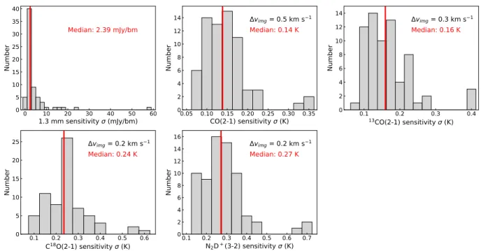
Figure 1. Subcompact configuration sensitivities for the imaged continuum and spectral line data. The median of each distribution is marked with a vertical red line. The imaged velocity resolution (∆vimg) for each spectral line is indicated in the
figure. Note that the 1.3 mm continuum sensitivity is often limited by dynamic range, such as Per-emb-12 (NGC 1333 IRAS4A), which is the histogram bar at 58 mJy bm−1.
per sideband chunk s13), 13CO(2–1), C18O(2–1), and
N2D+(3–2) were exported with their full resolution,
while the rest of the chunks were averaged together to generate the 1.3 mm continuum. For SWARM, which has uniform spectral resolution across the entire spec-trum, the data was exported in its entirety in MIRIAD. Lines were then split out of the bandwidth manually
us-ing MIRIAD, and the rest of the channels were averaged as continuum. In some cases, other high signal-to-noise spectral lines (besides the four mentioned above) were serendipitously detected with SWARM (Table 3), and thus were also removed from the continuum.
Table 5. Detection and Contour Information
1.3 mm Contoursb CO(2–1) Blue Contoursb CO(2–1) Red Contoursb
Contour Levels Contour Levels Velocity Range Contour Levels Velocity Range
Source Tracer Detected Toward Field?a [start, step] [start, step] [v
min,vmax] [start, step] [vmin,vmax]
Name 1.3 mm CO 13CO C18O N
2D+ (mJy bm−1) (Jy bm−1km s−1) (km s−1) (Jy bm−1km s−1) (km s−1)
Per-emb-1 Y Y Y Y Y [13, 20] [3, 5] [–13.5, 6.5] [6.6, 10] [10.5, 48.5]
Per-emb-2 Y Y Y Y Y [25, 50] [1.4, 1.4] [–1.6, 4.4] [2, 2] [8.9, 16.9]
Per-emb-3 Y Y Y Y Y [10, 10] [3, 1] [3.1, 3.6] [2.5, 2.5] [11.1, 19.1]
Per-emb-4 N Y Y Y N [5, 2] [0.4, 0.2] [2.5, 3.5] [1, 1] [11.5, 14.5]
Per-emb-5 Y Y Y Y Y [12, 24] [2.6, 2.6] [-11, 4] [3.7, 3.7] [10, 33]
Per-emb-6 Y Y Y Y Y [3.5, 2] [3.1, 1.5] [–3.35, 4.65] [2.8, 2.5] [9.65, 18.65]
Per-emb-7 Y Y Y Y Y [2.2, 1] [0.5, 0.25] [0, 2] [0.65, 0.3] [7, 9]
Per-emb-8 Y Y Y Y Y [6, 10] [1.4, 0.7] [4.65, 6.65] [1.8, 1.8] [12.65, 17.15]
Per-emb-9 Y Y Y Y Y [7.5, 5] [0.9, 0.9] [3.65, 6.15] [1.3, 1.3] [10.65, 14.65]
Per-emb-10 Y Y Y Y Y [4.5, 2] [1.5, 1.5] [–15.85, 5.65] [2.2, 2] [7.65, 37.15]
Per-emb-11 Y Y Y Y Y [18, 50] [1.5, 2.2] [–5.35, 5.65] [5, 5] [11.15, 25.15]
Per-emb-12 Y Y Y Y Y [200, 300] [9, 20] [–24.6, 3.9] [12, 20] [10.4, 46.4]
Per-emb-13 Y Y Y Y Y [80, 120] [16, 10] [–14.1, 4.9] [5, 5] [10.4, 25.4]
Per-emb-14 Y Y Y Y Y [25, 25] [0.6, 0.2] [1.5, 3] [6.2, 2] [13, 35.5]
Table 5(continued)
1.3 mm Contoursb CO(2–1) Blue Contoursb CO(2–1) Red Contoursb
Contour Levels Contour Levels Velocity Range Contour Levels Velocity Range
Source Tracer Detected Toward Field?a [start, step] [start, step] [vmin,vmax] [start, step] [vmin,vmax]
Name 1.3 mm CO 13CO C18O N2D+ (mJy bm−1) (Jy bm−1km s−1) (km s−1) (Jy bm−1km s−1) (km s−1)
Per-emb-15 Y Y Y Y Y [8, 4] [8, 4] [–18.35, 4.65] [1.4, 1] [11.15, 19.15]
Per-emb-16 Y Y Y Y Y [6, 4] [1.3, 3.7] [0.4, 6.4] [1, 1.5] [11.4, 14.9]
Per-emb-17 Y Y Y Y Y [7.5, 7.5] [1.7, 1.7] [–2.85, 0.65] [2.3, 2] [7.65, 9.15]
Per-emb-18 Y Y Y Y Y [15, 15] [7, 7] [–15.1, 1.4] [14, 6] [10.9, 24.4]
Per-emb-19 Y Y Y Y Y [5, 2] [1.2, 1.2] [3.65, 7.15] [0.37, 0.37] [10.15, 12.15]
Per-emb-20 Y Y Y Y Y [5, 2] [3.1, 3.1] [–5.35, 3.65] [2.7, 2.7] [7.65, 17.15]
Per-emb-21 Imaged in the same field as Per-emb-18
Per-emb-22 Y Y Y Y Y [16, 20] [8, 5] [–32.9, –0.9] [4.1, 5] [8.1, 23.6]
Per-emb-23 Y Y Y Y Y [5, 2.5] [2.1, 2.1] [3.65, 6.65] [0.6, 0.8] [10.15, 12.65]
Per-emb-24 M Y Y Y N [5.5, 2] [1.9, 1.9] [0.65, 5.65] [1.4, 1.4] [11.65, 15.65]
Per-emb-25 Y Y Y Y M [10, 10] [1.2, 1.2] [0.65, 3.65] [2, 1] [6.15, 9.15]
Per-emb-26 Y Y Y Y Y [13, 30] [13, 13] [–59.6, 2.4] [16, 16] [7.4, 44.9]
Per-emb-27 Y Y Y Y Y [30, 50] [5.4, 5.4] [–19.5, 1.5] [6, 6] [11.5, 22.5]
Per-emb-28 Imaged in the same field as Per-emb-16
Per-emb-29 Y Y Y Y Y [15, 20] [7, 7] [–12.2, 3.8] [5, 5] [10.3, 23.3]
Per-emb-30 Y Y Y Y Y [4, 6] [3, 2] [–2.5, 4] [1.2, 1] [11, 15.5]
Per-emb-31 N Y Y Y N [4, 2] [1.7, 1.7] [2.15, 6.15] [0.5, 0.5] [9.15, 17.15]
Per-emb-32 M Y Y Y N [6, 2] [0.5, 0.5] [3.65, 5.65] [2.5, 2.5] [10.15, 13.65]
Per-emb-33 Y Y Y Y Y [40, 100] [14, 14] [–45.1, 1.9] [6.5, 6.5] [7.4, 29.9]
Per-emb-34 Y Y Y Y N [2.2, 2] [7.6, 7.6] [–32.5, 5.5] [4.8, 4.8] [8, 38]
Per-emb-35 Y Y Y Y N [8, 8] [2.2, 2.2] [1.65, 6.15] [4, 2] [9.65, 15.65]
Per-emb-36 Y Y Y Y N [15, 15] [6, 4] [–10.35, 4.65] [14, 8] [10.65, 29.65]
Per-emb-37 Y Y Y Y N [4.6, 3] [1.1, 0.5] [2.65, 5.65] [0.7, 0.5] [11.15, 14.15]
Per-emb-38 Y Y Y Y N [3, 2] [0.3, 0.2] [1.5, 2.5] [0.52, 0.52] [8.5, 11.5]
Per-emb-39 Y Y Y M Y [3, 1] [0.3, 0.1] [2, 3] [0.3, 0.1] [12.5, 13.5]
Per-emb-40 Y Y Y Y N [6.5, 6.5] [10, 20] [–18.35, 4.65] [1.3, 1.3] [9.15, 14.15]
Per-emb-41 Y Y Y Y Y [20, 40] [1.1, 1.1] [–1.6, 4.4] [3.5, 3.5] [8.9, 12.9]
Per-emb-42 Imaged in the same field as Per-emb-26
Per-emb-43 N Y Y Y N [2, 0.8] [0.5, 0.3] [3.5, 4.5] [0.25, 0.1] [11, 12]
Per-emb-44 Y Y Y Y Y [50, 70] [30, 40] [–153, 5.5] [28, 28] [11.5, 164]
Per-emb-45 N Y Y Y N [5, 2] [0.3, 0.1] [1.15, 2.15] [0.67, 0.2] [10.15, 11.15]
Per-emb-46 Y Y Y Y N [5.1, 1.3] [1.2, 1.6] [–0.35, 4.15] [1, 0.5] [6.15, 7.15]
Per-emb-47 Y Y Y Y N [2, 2] [0.3, 0.08] [–0.5, 0.5] [1.3, 1.3] [14.5, 17.5]
Per-emb-48 M Y Y Y N [6, 3] [1, 0.5] [–0.85, 2.65] [0.4, 0.2] [13.65, 14.65]
Per-emb-49 Y Y Y Y Y [15, 15] [8, 8] [–13.85, 5.15] [5, 4] [11.15, 20.15]
Per-emb-50 Y Y Y Y N [8, 16] [5, 4] [–0.7, 4.8] [3, 2] [11.3, 19.3]
Per-emb-51 Y Y Y M Y [7.5, 7.5] [0.5, 0.1] [1.65, 2.65] [0.35, 0.1] [11.65, 12.65]
Per-emb-52 M Y Y Y Y [6, 2] [0.9, 0.9] [6.15, 7.15] [0.9, 0.9] [10.15, 12.65]
Per-emb-53 Y Y Y Y Y [7, 5] [4.5, 5] [–18.8, 8.2] [6, 8] [11.7, 34.7]
Per-emb-54 Y Y Y Y Y [15, 15] [5, 8] [–12.85, 2.65] [1.9, 1.9] [14.15, 20.65]
Per-emb-55 Imaged in the same field as Per-emb-8
Per-emb-56 Y Y Y Y N [7, 2] [0.8, 0.6] [2.65, 7.65] [0.7, 0.6] [13.15, 17.65]
Per-emb-57 Y Y Y Y N [4.5, 4.5] [1.1, 1.1] [2.65, 4.65] [0.34, 0.15] [13.15, 14.65]
Per-emb-58 Y Y Y Y Y [4.5, 2] [0.23, 0.1] [2.65, 3.65] [1.3, 0.5] [10.65, 11.15]
Per-emb-59 N Y Y M N [4, 1] [0.2, 0.1] [2.65, 3.65] [0.2, 0.1] [9.15, 10.15]
Per-emb-60 M Y Y Y N [3.3, 1.5] [1, 1] [2.15, 5.15] [0.25, 0.2] [12.15, 14.15]
Per-emb-61 Y Y Y Y N [6, 2] [0.75, 0.5] [5.65, 7.65] [1.5, 1.5] [11.15, 14.15]
Per-emb-62 Y Y Y Y N [5, 15] [0.32, 0.32] [5.15, 6.15] [2, 6] [10.65, 19.65]
Per-emb-63 Y Y Y Y N [7.5, 3] [0.7, 0.5] [0.65, 3.65] [1, 1] [11.15, 13.15]
Per-emb-64 Y Y Y Y N [5, 5] [0.5, 0.3] [3.65, 4.15] [1.3, 0.5] [11.15, 17.15]
Per-emb-65 Y Y Y Y N [3, 3] [0.12, 0.12] [3.15, 3.65] [0.17, 0.17] [11.65, 12.65]
Per-emb-66 N Y Y Y N [2, 1] [0.7, 0.5] [3, 5.5] [1, 1] [10, 12.5]
Stephens et al.
Table 5(continued)
1.3 mm Contoursb CO(2–1) Blue Contoursb CO(2–1) Red Contoursb
Contour Levels Contour Levels Velocity Range Contour Levels Velocity Range
Source Tracer Detected Toward Field?a [start, step] [start, step] [vmin,vmax] [start, step] [vmin,vmax]
Name 1.3 mm CO 13CO C18O N2D+ (mJy bm−1) (Jy bm−1km s−1) (km s−1) (Jy bm−1km s−1) (km s−1)
B1bN Y Y Y Y Y [17, 40] [1.7, 1.7] [–1.6, 4.4] [1.3, 0.5] [8.9, 13.4]
B1bS Imaged in the same field as Per-emb-41
L1448IRS2E N Y Y Y M [8, 4] [0.4, 0.1] [–3.9, –2.4] [9, 9] [6.6, 35.6]
L1451-MMS Y Y Y Y Y [8, 8] [0.39, 0.39] [3, 4] [0.6, 0.3] [5, 7]
Per-bolo-45 Y Y Y Y Y [5, 2] [0.7, 0.2] [2.65, 4.15] [4.5, 4.5] [11.15, 26.65]
Per-bolo-58 Y Y Y Y Y [4.5, 2] [0.9, 0.2] [3.8, 6.8] [0.3, 0.2] [10.8, 12.3]
SVS 13B Imaged in the same field as Per-emb-44
SVS 13C Y Y Y Y Y [35, 35] [7.5, 7.5] [108.5, 7] [8, 8] [11.5, 61]
aAnswers are: (Y)es, (N)o, or (M)arginal. Although CO(2–1),13CO(2–1), and C18O(2–1) are essentially detected toward every field, it does not
mean that the line is associated with the protostar. Large-scale emission from the Perseus molecular cloud is frequently detected with the SMA even when emission is not associated with the protostar.
bThese contours are those shown in Figure3.
3.2. Imaging
All targets of the MASSES survey were imaged with MIRIAD after exporting the calibrated data from MIR. For imaging of spectral lines, we first used the MIRIAD taskuvlinto subtract a 0th order polynomial from the continuum. The delivered spectral lineuvdata all have had their continuum subtracted.
Dirty maps were then created via an inverse Fourier transform using the MIRIAD taskinvert. If a particu-lar target was observed over multiple days (see Table1), the tracks were combined during this task. All targets were imaged using Briggs weighting with the robust pa-rameter equal to 1. We also specified the pixel size to be 000.8 with 100 pixels on each side of the map, resulting in 8000×8000 maps. These maps image outside the full width at half maximum (FWHM) of the primary beam, which has a size of 4800at 231 GHz. For each line, we also specified the imaged channel width, which was slightly wider than the channel spectral resolution. The imaged spectral resolutions are specified in Table 2 under the ∆vimgcolumn. The number of channels imaged are also listed in this table. For CO(2–1) data, which often have high velocity components, an additional ASIC chunk is available in the upper sideband (s13). This chunk pro-vides for red-shifted velocities of ∼26–160 km s−1, but
the user should note that for many targets, the noise in the chunk is extremely high at the edges. The s13 chunk has a slight overlap with the main CO(2–1) chunk, s14, which is imaged for velocities up to∼48.5 km s−1. In the
case that the CO(2–1) data was imaged with SWARM, we imaged channels for a larger velocity range (as indi-cated in Table2) than that which can done with a single ASIC chunk.
After creating dirty maps, we cleaned the maps using the MIRIAD taskclean. For CO(2–1) and 13CO(2–1),
which typically trace protostellar outflows, we used a three-step iterative cleaning algorithm. We first cleaned only the pixels and channels with emission to a level of 1.5 times the dirty map noise. This was completed by binning channels together with similar emission and making multiple regions with the task cgcurs. When selecting such pixels and channels, we typically excluded emission near the systemic velocity since the emission is often completely confused with the large scale emission of the Perseus molecular cloud. For the second step, we selected the area withcgcurswhere emission is present over the entire cube, and cleaned this entire region for all channels to 2 times the dirty map noise. For the third and final step, we cleaned over all pixels and channels to 2.5 times the dirty map noise. We find that this three-step cleaning process recovers the extended emission well while minimizing the creation of interferometric imaging artifacts.
For the continuum, C18O(2–1), and N
2D+(3–2), all of
which typically trace protostellar envelopes, we used a two-step iterative cleaning algorithm. This algorithm is identical to that described above, except we skip the second step since the step had a negligible effect for imaging the compact emission that is usually found by these three tracers. For both the three-step and two-step cleaning processes, if no emission was obviously as-sociated with a source, we only cleaned the channels to 3 times the dirty map noise. After deriving the clean components, we used the MIRIAD taskrestor to cre-ate clean maps.
the continuum was measured using the IDL task sky.4
This task measures the standard deviation over the en-tire map, clips all values deviating from 3 times this standard deviation, and iteratively repeats this for a to-tal of 5 iterations. Sensitivities for the continuum were often limited by dynamic range rather than integration time. For some sources, self-calibration may help the continuum sensitivity, but we choose to not self-calibrate because we want to deliver consistent data products to the user. We note that sensitivity improvements us-ing self-calibration with the SMA is typically minimal (i.e., less than∼10%), in part because the SMA is only an eight element array. Note that the uv data is pro-vided in case the user wants to apply the calibration. For the sensitivity of spectral line observations, we mea-sured the standard deviation of the pixels over many emission-free channels and converted the standard devi-ation to a brightness temperature. The distribution of sensitivities are shown in Figure1.
The sensitivity of the continuum observations are fre-quently limited by dynamic range. Figure 2 shows the peak 1.3 mm pixel flux normalized by the sensitivity (a proxy for dynamic range) versus the sensitivity of the image. Targets that have higher dynamic range have worse sensitivities, even for good observing conditions, indicating that continuum sensitivities are often limited by dynamic range.
10
010
0.510
110
1.510
2Sensitivity (mJy/bm)
10
20
30
40
50
60
Peak flux/Sensitivity
Figure 2. Peak pixel flux of a 1.3 mm continuum image divided by the sensitivity (σ1.3 mm) of the image, versus the
sensitivity of the image (σ1.3 mm). The continuum sensitivity
is frequently limited by dynamic range.
Table 4 also gives the FWHM of the synthesized beam’s major and minor axes,θmaj, and θmin, and the position angle of the beam’s major axis, PA, which is measured counterclockwise (east) from north.
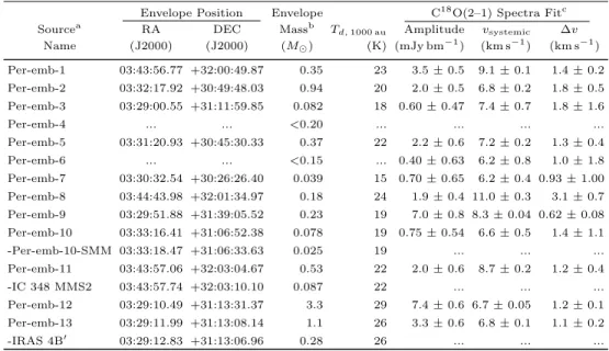
Table 6. Envelope masses, Dust Temperatures, and C18O(2–1) Fitting Information
Envelope Position Envelope C18O(2–1) Spectra Fitc
Sourcea RA DEC Massb Td,1000 au Amplitude vsystemic ∆v
Name (J2000) (J2000) (M) (K) (mJy bm−1) (km s−1) (km s−1)
Per-emb-1 03:43:56.77 +32:00:49.87 0.35 23 3.5±0.5 9.1±0.1 1.4±0.2
Per-emb-2 03:32:17.92 +30:49:48.03 0.94 20 2.0±0.5 6.8±0.2 1.8±0.5
Per-emb-3 03:29:00.55 +31:11:59.85 0.082 18 0.60±0.47 7.4±0.7 1.8±1.6
Per-emb-4 ... ... <0.20 ... ... ... ...
Per-emb-5 03:31:20.93 +30:45:30.33 0.37 22 2.2±0.6 7.2±0.2 1.3±0.4
Per-emb-6 ... ... <0.15 ... 0.40±0.63 6.2±0.8 1.0±1.8
Per-emb-7 03:30:32.54 +30:26:26.40 0.039 15 0.70±0.65 6.2±0.4 0.93±1.00
Per-emb-8 03:44:43.98 +32:01:34.97 0.18 24 1.9±0.4 11.0±0.3 3.1±0.7
Per-emb-9 03:29:51.88 +31:39:05.52 0.23 19 7.0±0.8 8.3±0.04 0.62±0.08
Per-emb-10 03:33:16.41 +31:06:52.38 0.078 19 0.75±0.54 6.6±0.5 1.4±1.1
-Per-emb-10-SMM 03:33:18.47 +31:06:33.63 0.025 19 ... ... ...
Per-emb-11 03:43:57.06 +32:03:04.67 0.53 22 2.0±0.6 8.7±0.2 1.2±0.4
-IC 348 MMS2 03:43:57.74 +32:03:10.10 0.087 22 ... ... ...
Per-emb-12 03:29:10.49 +31:13:31.37 3.3 29 7.4±0.6 6.7±0.05 1.2±0.1
Per-emb-13 03:29:11.99 +31:13:08.14 1.1 26 3.3±0.6 6.8±0.1 1.1±0.2
-IRAS 4B0 03:29:12.83 +31:13:06.96 0.28 26 ... ... ...
Table 6 continued
4 Available in the IDL Astronomy User’s Library, https://
Stephens et al.
Table 6(continued)
Envelope Position Envelope C18O(2–1) Spectra Fitc
Sourcea RA DEC Massb Td,1000 au Amplitude vsystemic ∆v
Name (J2000) (J2000) (M) (K) (mJy bm−1) (km s−1) (km s−1)
Per-emb-14 03:29:13.52 +31:13:57.75 0.16 19 1.4±0.5 7.7±0.3 1.8±0.7
Per-emb-15 03:29:04.19 +31:14:48.43 0.12 18 1.2±0.5 6.5±0.3 1.6±0.8
Per-emb-16 03:43:51.00 +32:03:23.86 0.14 18 1.7±0.6 8.5±0.2 1.1±0.5
Per-emb-17 03:27:39.12 +30:13:02.53 0.10 26 1.6±0.5 5.8±0.3 1.8±0.6
Per-emb-18 03:29:11.26 +31:18:31.33 0.21 25 3.7±0.5 8.1±0.1 1.6±0.2
Per-emb-19 03:29:23.48 +31:33:28.94 0.022 17 1.7±0.6 7.5±0.2 1.0±0.4
-Per-emb-19-SMM 03:29:24.33 +31:33:22.57 0.011 17 ... ... ...
Per-emb-20 03:27:43.20 +30:12:28.96 0.061 22 2.2±0.6 5.1±0.1 0.98±0.33
-Per-emb-20-SMM 03:27:42.78 +30:12:25.94 0.017 22 ... ... ...
Per-emb-21 03:29:10.69 +31:18:20.15 0.19 25 1.7±0.5 8.7±0.2 1.7±0.6
Per-emb-22 03:25:22.35 +30:45:13.21 0.37 26 3.6±0.6 3.9±0.1 1.3±0.2
Per-emb-23 03:29:17.25 +31:27:46.34 0.098 20 3.5±0.6 7.6±0.09 1.1±0.2
Per-emb-24 ... ... <0.25 ... 0.99±0.61 7.6±0.3 1.1±0.8
Per-emb-25 03:26:37.49 +30:15:27.90 0.10 21 1.5±0.7 5.5±0.2 0.75±0.43
Per-emb-26 03:25:38.87 +30:44:05.30 0.37 30 3.1±0.5 5.1±0.1 1.4±0.3
Per-emb-27 03:28:55.56 +31:14:37.17 0.47 34 3.1±0.5 7.8±0.1 1.9±0.3
Per-emb-28 03:43:50.99 +32:03:07.97 0.086 18 0.65±0.59 8.4±0.5 1.1±1.2
Per-emb-29 03:33:17.86 +31:09:32.31 0.43 26 3.5±0.6 6.1±0.09 1.1±0.2
Per-emb-30 03:33:27.33 +31:07:10.29 0.074 23 2.2±0.5 7.1±0.2 1.6±0.4
Per-emb-31 ... ... <0.18 ... 0.43±0.42 7.2±1.1 2.3±2.6
Per-emb-32 ... ... <0.22 ... 1.2±0.6 9.4±0.3 1.0±0.6
Per-emb-33 03:25:36.32 +30:45:14.77 0.82 29 2.0±0.4 4.9±0.2 2.1±0.5
-L1448IRS3 03:25:35.68 +30:45:35.16 0.26 29 ... ... ...
-L1448NW 03:25:36.46 +30:45:21.43 0.17 29 ... ... ...
Per-emb-34 03:30:15.19 +30:23:49.11 0.024 23 1.4±0.5 6.1±0.3 1.4±0.6
Per-emb-35 03:28:37.12 +31:13:31.24 0.097 30 3.4±0.6 7.2±0.1 1.3±0.2
Per-emb-36 03:28:57.36 +31:14:15.61 0.19 27 2.2±0.4 7.0±0.2 2.2±0.5
Per-emb-37 03:29:18.94 +31:23:13.11 0.082 18 ... ... ...
Per-emb-38 03:32:29.22 +31:02:42.73 0.044 19 0.92±0.56 7.0±0.4 1.3±0.9
Per-emb-39 ... ... ?d ... ... ... ...
Per-emb-40 03:33:16.65 +31:07:54.81 0.028 22 2.0±0.4 7.1±0.2 2.0±0.5
Per-emb-41 ... ... <0.54 ... ... ... ...
Per-emb-42 ... ... <0.45e ... 1.4±0.5 5.5±0.3 1.4±0.6
Per-emb-43 ... ... <0.075 ... ... ... ...
Per-emb-44 03:29:03.76 +31:16:03.43 0.38 38 4.4±0.4 8.4±0.1 2.0±0.2
Per-emb-45 ... ... <0.20 ... ... ... ...
Per-emb-46 ... ... <0.18 ... 0.38±0.58 5.1±0.9 1.2±2.1
Per-emb-47 03:28:33.87 +31:00:52.49 0.016 22 1.1±0.6 7.4±0.3 1.0±0.7
Per-emb-48 ... ... <0.28 ... ... ... ...
Per-emb-49 ... ... <0.44 ... ... ... ...
Per-emb-50 03:29:07.76 +31:21:57.16 0.062 35 1.4±0.6 7.4±0.3 1.3±0.6
Per-emb-51 03:28:34.52 +31:07:05.47 0.25 13 0.52±0.52 6.7±0.7 1.5±1.7
Per-emb-52 ... ... ?d ... 0.99±0.83 7.9±0.2 0.58±0.56
Per-emb-53 03:47:41.58 +32:51:43.75 0.065 27 2.9±0.5 10.0±0.1 1.5±0.3
Per-emb-54 03:29:02.83 +31:20:41.32 0.13 33 8.5±0.5 8.0±0.04 1.5±0.1
Per-emb-55 ... ... <0.23e ... ... ... ...
Per-emb-56 03:47:05.42 +32:43:08.33 0.019 19 0.76±0.72 11.0±0.4 0.76±0.84
Per-emb-57 03:29:03.32 +31:23:14.34 0.048 14 ... ... ...
Per-emb-58 03:28:58.36 +31:22:16.81 0.010 19 2.8±0.9 8.0±0.08 0.46±0.18
Per-emb-59 ... ... <0.18 ... ... ... ...
Per-emb-60 ... ... ?d ... ... ... ...
Per-emb-61 03:44:21.30 +31:59:32.53 0.019 16 1.0±0.5 9.5±0.3 1.3±0.8
Per-emb-62 03:44:12.97 +32:01:35.29 0.080 23 1.2±0.8 8.3±0.2 0.56±0.47
Table 6(continued)
Envelope Position Envelope C18O(2–1) Spectra Fitc
Sourcea RA DEC Massb Td,1000 au Amplitude vsystemic ∆v
Name (J2000) (J2000) (M) (K) (mJy bm−1) (km s−1) (km s−1)
Per-emb-63 03:28:43.28 +31:17:33.25 0.019 23 ... ... ...
Per-emb-64 03:33:12.85 +31:21:23.95 0.043 25 ... ... ...
Per-emb-65 03:28:56.30 +31:22:27.69 0.049 15 ... ... ...
Per-emb-66 ... ... <0.090 ... ... ... ...
B1bN 03:33:21.20 +31:07:43.93 0.38 17 ... ... ...
B1bS 03:33:21.34 +31:07:26.44 0.38 24 ... ... ...
L1448IRS2E ... ... <0.27 ... ... ... ...
L1451-MMS 03:25:10.24 +30:23:55.01 0.092 12 0.20±0.47 7.5±2.0 1.8±4.8
Per-bolo-45 03:29:06.77 +31:17:29.96 0.16 13 ... ... ...
Per-bolo-58 03:29:25.42 +31:28:14.21 0.22 12 0.48±0.61 8.1±0.7 1.1±1.6
SVS 13B 03:29:03.08 +31:15:50.98 0.86 21 3.3±0.6 8.3±0.09 0.95±0.22
SVS 13C 03:29:02.03 +31:15:37.75 0.20 23 3.4±0.5 8.7±0.1 1.9±0.3
aAnswers are: (Y)es, (N)o, or (M)arginal. Although CO(2–1),13CO(2–1), and C18O(2–1) are essentially detected toward every field, it does
not mean that the line is associated with the protostar. Large-scale emission from the Perseus molecular cloud is frequently detected with the SMA even when emission is not associated with the protostar.
bThese contours are those shown in Figure3.
Table5shows whether the line is detected toward each MASSES field, as judged by analyzing the continuum images and the spectral cubes by eye. With the excep-tion of some marginal C18O(2–1) detections, the three
spectral lines CO(2–1), 13CO(2–1), and C18O(2–1) are
detected toward every field. Nevertheless, these detec-tions do not imply that the emission is always associ-ated with the source since the large-scale emission of the Perseus molecular cloud is detected with these ob-servations. Indeed, spectral lines do not seem to be asso-ciated with many of the targets, which will be analyzed in more detail in Section5.5.
3.3. Continuum Mass Detection Limit
We estimate the minimum mass of a compact source that we expect to detect for a given continuum observa-tions based on the measured sensitivityσ1.3 mm.
Follow-ingHildebrand(1983), the mass of a source for optically thin dust continuum flux is
M =Rgd
Fνd2
κνBν(Tdust)
, (1)
where Rgd is the gas to dust mass ratio, Fν is the source’s flux, d is the distance to the source, κν is the dust opacity, and Bν(Tdust) is the Planck function
at dust temperature Tdust. We assume typical values
of Rgd = 100, d = 235 pc (Hirota et al. 2008), and κ1.3 mm= 0.899 cm2g−1(Ossenkopf & Henning 1994,
as-suming thin ice mantles and a gas density of 106cm−3).
To be conservative with our minimum detected compact mass estimates, we assume Tdust = 10 K and require a
three-sigma detection with all the flux in a single beam,
i.e., Fν = 3(σ1.3 mm×bm). Note that if the source is
larger than the beam, this assumption forFνis not valid, i.e., we are only concerned with the detection limit of a source smaller than the beam. Given these assumptions, the mass detection limit for each field is
Mlimit=
σ
1.3 mm
mJy bm−1
×0.010M, (2)
where σ1.3 mm is given in Table 4. The mass
sensitiv-ity for the continuum varies dramatically, often due to dynamic range, but also due to observing conditions and the correlator that is used (ASIC vs. SWARM). To demonstrate a pessimistic mass detection limit for the majority of the observations, we select the observa-tion for Per-emb-4 as an illustrative example. In this field, no continuum source was detected (i.e., we were not limited by dynamic range), and our estimated ther-mal noise is a bit worse than most MASSES observations due to unfavorable observing conditions. For this field,
σ1.3 mm = 2.0 mJy bm−1, soMlimit = 0.02M. There-fore, for most of our fields, we expect to detect a compact source greater than 0.020M with >3σ significance, if it exists.
Many sources in Table4 haveσ1.3 mm values that are
much higher than 2.0 mJy bm−1 because these observa-tions were limited by dynamic range. In other words, while our detection limit is generally∼0.02M, if there is a much brighter source in the field, we would not be able to detect a 0.02M source in the same field.
4. DELIVERABLES
Stephens et al.
directly fromhttps://dataverse.harvard.edu/dataverse/ MASSES. The MASSES Dataverse contains two sep-arate datasets for each observed source. One dataset contains uv data while the other dataset contains im-ages/cubes for the continuum and line observations. For each dataset, we include a README file that briefly summarizes the contents and explains how to use the dataset.
As mentioned in Section2.2and Table2, the CO(2–1) line uses two chunks in the upper sideband, with the majority of the spectral line in the s14 chunk. The de-liverables refer to the s14 chunk as the “12CO21” chunk and the s13 chunk as the “highvelCO” chunk.
4.1. uv data
We provide the delivered uv data for both the con-tinuum observations and spectral line observations. If tracks were taken on the same day (i.e., had the same YYMMDD prefix; see Section 2.2), they are combined into a single dataset during the MIR calibration. As ex-plained in Section3.2, lines were subtracted when gener-ating the continuum, and the continuum was subtracted for each spectral line observation. The line uv data is delivered per spectral line for each track, while the con-tinuumuvdata is delivered separately for the lower and upper sideband.
Finally, for the SWARM data, we also provide the full resolutionuv data, which is not continuum-subtracted. Many additional spectral lines (Table 3) may be found in these cubes, as discussed in Section 2.2. These lines were typically not detected in the ASIC cubes in part due to the smaller bandwidth coverage, although the coarse spectral resolution also makes such detections with ASIC less obvious. These SWARM uv data are delivered separately for each of its 8 (4 per sideband) spectral chunks.
We also note that toward the edge of both SWARM and ASIC chunks, the noise in the spectra is extremely high, so the user should use these channels with caution. These channels were not used for the delivered imaged cubes.
Theuvdata are delivered as uv-fits files. Examples of the delivered uv-fits filenames are given in Section4.3.
4.2. Imaged data
For the continuum and spectral line observations, we deliver both the images not corrected for the primary beam as well as the primary-beam corrected images. The images that are not corrected for the primary beam are typically used to better show structure throughout the entire map. The primary-beam corrected images al-low the user to make accurate flux measurements.
Multiple tracks were combined during the MIRIAD
invert task (Section 3.2), allowing for two delivered products per continuum/spectral line (primary beam uncorrected and corrected). These data are delivered as fits files.
The units for the continuum images are Jy bm−1, and
the units for the spectral line cubes are Jy bm−1channel−1.
4.3. Examples of Delivered Data
An example of the delivered fits files for the Per-emb-24 dataset is shown below.
The delivereduv data for Per-emb-24 are: • Per24.sub.cont1.3mm.lsb.151122.uvfits • Per24.sub.cont1.3mm.usb.151122.uvfits • Per24.sub.cont1.3mm.lsb.151127.uvfits • Per24.sub.cont1.3mm.usb.151127.uvfits • Per24.sub.12CO21.151122.uvfits • Per24.sub.12CO21.151127.uvfits • Per24.sub.highvelCO.151122.uvfits • Per24.sub.highvelCO.151127.uvfits • Per24.sub.13CO21.151122.uvfits • Per24.sub.13CO21.151127.uvfits • Per24.sub.C18O21.151122.uvfits • Per24.sub.C18O21.151127.uvfits • Per24.sub.N2DP.151122.uvfits • Per24.sub.N2DP.151127.uvfits
The delivered images/data cubes for Per-emb-24 are: • Per24.sub.cont1.3mm.fits
• Per24.sub.cont1.3mm.pbcor.fits • Per24.sub.12CO21.cube.fits • Per24.sub.12CO21.cube.pbcor.fits • Per24.sub.highvelCO.cube.fits • Per24.sub.highvelCO.cube.pbcor.fits • Per24.sub.13CO21.cube.fits
• Per24.sub.13CO21.cube.pbcor.fits • Per24.sub.C18O21.cube.fits • Per24.sub.C18O21.cube.pbcor.fits • Per24.sub.N2DP.cube.fits
• Per24.sub.N2DP.cube.pbcor.fits
Tracks with SWARM data will include include addi-tional full spectral resolutionuv data, separated into 8 chunks (4 for each sideband). An example of the addi-tional SWARMuvdata for Per-emb-7 is shown below.
-30 -15 0 15 30
Dec offset (arcsec) 4000 AU
-30 -15 0 15 30
Dec offset (arcsec)
Per8
Per55
Per6
Per13
Per12
-30 -15 0 15 30
Dec offset (arcsec)
Per16 Per28
Per18
Per21
-30 -15 0 15 30
Dec offset (arcsec)
Per26 Per42
Per36
-30 -15 0 15 30
Dec offset (arcsec)
Per27
-30 -15 0 15 30
Dec offset (arcsec)
B1bN
B1bS Per41
Per44
SVS 13B
-30 -15 0 15 30
Dec offset (arcsec)
Per18 Per21
-30 -15 0 15 30
Dec offset (arcsec)
-30 -15 0 15 30 RA offset (arcsec) -30
-15 0 15 30
Dec offset (arcsec)
-30 -15 0 15 30
RA offset (arcsec) -30 -15 0 15 30RA offset (arcsec) -30 -15 0 15 30RA offset (arcsec) -30 -15 0 15 30RA offset (arcsec) -30 -15 0 15 30RA offset (arcsec) -30 -15 0 15 30RA offset (arcsec)
-30 -15 0 15 30 RA offset (arcsec) -30
-15 0 15 30
Dec offset (arcsec) B1bS
-30 -15 0 15 30
RA offset (arcsec) -30 -15 0 15 30RA offset (arcsec) -30 -15 0 15 30RA offset (arcsec) -30 -15 0 15 30RA offset (arcsec)
Per44 SVS13B