PARAMETER ESTIMATION IN NON-HOMOGENEOUS BOOLEAN MODELS: AN APPLICATION TO PLANT DEFENSE RESPONSE

PARAMETER ESTIMATION IN NON-HOMOGENEOUS BOOLEAN

MODELS: AN APPLICATION TO PLANT DEFENSE RESPONSE

M

´

A

´

G

M

´

V

I

´

˜

A

S

´

B

1_{Departament de Matem`atiques, Universitat Jaume I, Spain;</sub>2<sub>Departament de Matem`atiques-IMAC, Universitat}

Jaume I, Spain.

e-mail: [email protected]; [email protected]; [email protected]

(Received October 28, 2013; revised May 23, 2014; accepted September 23, 2014)

ABSTRACT

Many medical and biological problems require to extract information from microscopical images. Boolean models have been extensively used to analyze binary images of random clumps in many scientific fields. In this paper, a particular type of Boolean model with an underlying non-stationary point process is considered. The intensity of the underlying point process is formulated as a fixed function of the distance to a region of interest. A method to estimate the parameters of this Boolean model is introduced, and its performance is checked in two different settings. Firstly, a comparative study with other existent methods is done using simulated data. Secondly, the method is applied to analyze thelongleaf data set, which is a very popular data set in the context of point processes included in the R packagespatstat. Obtained results show that the new method provides as accurate estimates as those obtained with more complex methods developed for the general case. Finally, to illustrate the application of this model and this method, a particular type of phytopathological images are analyzed. These images show callose depositions in leaves of Arabidopsis plants. The analysis of callose depositions, is very popular in the phytopathological literature to quantify activity of plant immunity. Keywords: binary images, callose deposition, mixed volumes, non-homogeneous Boolean model, parameter estimation.

INTRODUCTION

In a wide variety of technological and scientific fields there are many practical situations in which researchers need to manage image data in order to obtain conclusions about a phenomenon of interest. Very often, these images are binary images showing the area covered by a given phenomenon in a certain region. A very appropriate probabilistic model for studying this kind of images, where the area covered by different events usually overlaps (random clumps),

is the Boolean model (Molchanov, 1997; Chiu et

al., 2013). This model is formed by placing random

compact sets on the points of a Poisson point process and considering the union of these sets. Difficulties arise when certain grains overlap or remain completely covered by the others, thus making it impossible to perform direct measurements of the characteristics of the particles.

A formal definition of a Boolean model is as follows.

Definition 1 (Boolean model) Let Φ_λ ={x1,x2, . . .}

be a stationary Poisson point process in IRdof intensity

λ. Let Ξ1,Ξ2, . . . be a sequence of independent

identically distributed random compact sets in IRdthat are independent of the Poisson processΦλ and satisfy Eνd(Ξ0⊕Kˇ)<+∞for all compacts K⊂IRd, where

Ξ0is a random compact set of the same distribution as Ξn,Kˇ ={−x:x∈K} andνd is the d−dimensional

Lebesgue measure. The Boolean model Ξ is then

defined as:

Ξ=[ i

(xi+Ξi). (1)

The points xi are called germs, the sets Ξi are

known asgrains and the random set Ξ0 is said to be

the typical grainof the Boolean model. The value of

parameterλ is said to be theintensityof the Boolean

model.

If the grains have an isotropic distribution (distribution that is invariant under rotations about the origin), then the Boolean model is also isotropic in distribution.

A more in-depth study of this model can be found in Serra (1982), Ayala (1988), Cressie (1993),

Molchanov (1997) and Chiuet al.(2013). Applications

of Boolean models to real images have been worked by Lyman (1972), Margalef (1974), Serra (1982), Plaza

(1991) and Chiuet al.(2013), among others.

non-homogeneous Boolean models have been studied by Molchanov and Chiu (2000) and by Schmitt (1996). Non-homogeneous Boolean models have been used for the functional modeling of graded materials

(Quintanilla and Torquato, 1997; Hahn et al., 1999),

distributions of galaxies (Bond et al., 1995) and

complex fluids (Brodatzki and Mecke, 2001).

Our aim in this paper is to propose an alternative statistical method to estimate the parameters of interest of a particular type of non-homogeneous Boolean model. This particular model can be applied to a great variety of practical situations. As an example, we will show its application to a phytopathological problem. Our method is similar in some respects to that of Berman and Turner (1992) for inhomogeneous point processes.

In this application, we will work with microscopic images obtained in the study of callose deposition

in leaves of Arabidopsis plants (Luna et al., 2011).

The study of callose deposition is a very popular method in the phytopathological literature to quantify plant immune system activity. Callose deposition in a leaf form random clumps, which are more densely distributed near the nerves of the leaf. So in this case, we can consider this deposition as a realization of a non-homogeneous Boolean model where the intensity of the Poisson point process is modeled as a known function of the distance from each point to the closest leaf nerve. As a result, a particular non-homogeneous Boolean model can be assumed. As an alternative to the method proposed by Schmitt (1996) and Molchanov and Chiu (2000), we propose, for this model, a parameter estimation method based on a least squares fit procedure applied to the area fraction and to the density of the boundary length functions.

The rest of the paper is organized as follows: first the definition of non-homogeneous Boolean model will be introduced. A particular case of this model will be detailed in the following section. Then the parameter estimation procedures proposed by Molchanov and Schmitt will be explained, together with a new estimation procedure that will be proposed. Next a simulation study will be carried out to test the performance of the different parameter estimation procedures. In the subsequent section the proposed method is applied to a very popular data set. This data

set is included in the R packagespatstatand provides

the locations and diameters of adult longleaf pines in a region. In this data set the germ process is known, so we can compare our results with those obtained using point process methods. Then this method will be applied to analyze microscopic images obtained in the

study of callose deposition in plant leaves (Lunaet al.,

2011). Finally, conclusions will be stated.

NON-HOMOGENEOUS BOOLEAN

MODEL

The assumption of stationarity in the definition of the Boolean model (Def. 1), means that the phenomenon being studied spreads over the plane in a homogeneous way. As has been stated previously, in practice this hypothesis usually fails, but it is still assumed as it facilitates the parameter estimation process.

In many real situations, where this hypothesis is not acceptable at all, a suitable model is the non-homogeneous Boolean model. A non-non-homogeneous

Boolean model (Molchanov, 1997; Chiuet al., 2013)

is a Boolean model whose germ process is a non-homogeneous Poisson point process that is obtained substituting the constant intensity of the homogeneous

Poisson process by a general intensity measureΛ(B),

for B⊂IRd. Usually Λ(B) =R

Bλ(x)dx. The density

λ(x), that is, finite and non-negative, is called the

intensity function of the general Poisson point process. The formal definition of a non-homogeneous Boolean model is as follows.

Definition 2 (Non-homogeneous Boolean model)

LetΦ_λ ={x1,x2, . . .}be a non-homogeneous Poisson

process in _Rd with intensity function λ(x). Let Ξ1,Ξ2, . . . be a sequence of independent identically

distributed random compact sets in IRd that are independent of the Poisson process Φλ and satisfy Eνd(Ξ0⊕Kˇ) <+∞ for all compacts K, where Ξ0

is a random compact set of the same distribution as

Ξn, andνd is the d−dimensional Lebesgue measure.

The non-homogeneous Boolean model (NHBM) Ξ is

Ξ=Si(xi+Ξi).

The points xi are called germs, the sets Ξi are

known as grains and the random set Ξ0 is referred

to as the typical grain. A non-homogeneous Boolean

model is characterized by its intensity function and the probability distribution of its typical grain. From now

on, we will continue working onR2i.e., fixingd=2.

Given a NHBM (Def. 2), its probability

distribution is characterized by its capacity functional,

which, for each compact setK, is defined as:

T_Ξ(K) =P(Ξ\K6=/0)

=1−exp[−E{Λ(K⊕_Ξˇ_{0)}], (2)}

The capacity functional for K = {x}, p(x) =

TΞ({x}) is defined as the volume fraction function,

in general, or as the area fraction function in the

particular case ofd=2. Therefore, by Eq. 2,

p(x) =P(x∈Ξ) =1−exp[−E{Λ(x⊕Ξˇ0)}],

and by Fubini’s theorem:

p(x) =1−exp[−E{

Z

ˇ Ξ

λ(x−y)dy}]. (3)

The area fraction function is a particular case

of the extended intrinsic volume densities ¯Vj(Ξ;x)

j=0,1,2 of the Boolean modelΞ. p(x) =V¯2(Ξ;x).

Another interesting extended intrinsic volume density

is ¯V1(Ξ;x)the density function of the boundary length,

denoted byLA(x). The density of the boundary length

of a NHMB at pointxis (Weil, 2001):

LA(x) = (1−p(x))E{

Z

R2

λ(x−y)Φ1(Ξ,dy)}, (4)

where Φ1(Ξ,dy) denotes the generalized curvature

measure ofΞ(Schneider and Weil, 2008). 2Φ1(Ξ,B)

is defined as the length of∂ΞTB, where∂Ξdenotes

the boundary ofΞandB⊂IR2is a Borel set.

Non-homogeneous Boolean models with spherical

grains in R2 and R3 have interesting applications

in statistical physics, in particular for continuous percolation problems.

Estimators of the area fraction function and the density of the boundary length can be found in Molchanov (1997). We have to note that the measurement of the density of the boundary length is not very easy to implement on the digitized computer.

A PARTICULAR CASE OF

NON-HOMOGENEOUS BOOLEAN

MODEL

Departure from the homogeneity hypothesis can be due to a large number of different causes. In particular, in this paper we are going to focus our interest on one of the most common causes in practice: the case where the phenomenon of interest is spread over the plane non-homogeneously, depending on the distance

to a certain focus or region of interest,ROI. Examples

include proliferation of houses and/or industries close to main roads in a country; plants affected by a virus around the outbreak of the disease; radioactivity levels or cases of illness around a power plant, a nuclear plant or particular industries; destruction around the

epicenter of an earthquake, and so on. In particular, in the example that we will analyze later, we will work with microscopic images of leaves, where callose deposition is non-homogeneously distributed across their surface, showing an intensity of events that depends on the proximity to the nerves of the leaves.

In order to take advantage of prior knowledge on the characteristics of the non-homogeneity, we suggest considering a particular NHBM with:

– A parametric intensity function λ(x) =

f(DROI(x);a), where f is a known function

depending on a= (a1, . . . ,ap), the parameters to

estimate, DROI(x) is the distance from point x to

the region of interest,ROI, and f(DROI(x);a)≥0

∀x∈R2.

– A parametric grain distribution. We assume that

the typical grain is a ball with a random radius whose probability distribution is known except for

some parameters.i.e.,Ξ0 =B(0,r), whereB(0,r)

denotes the ball centered in the origin and radius

r and r has the probability density g(r;θ), with

θ= (θ1, . . . ,θk).

Under these conditions, the area fraction function (Eq. 3) and the density of the boundary length (Eq. 4) become (Weil, 2001):

p(x) =1−

exp

−

ZZ

B(x,r)

f(DROI(y);a)g(r;θ)dydr

,

(5)

LA(x) = (1−p(x))· _Z

R2

f(DROI(x−y);a)g(kyk;θ)dy

. (6)

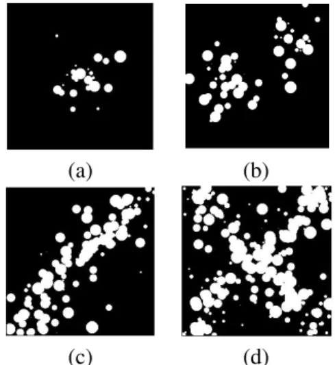
As an illustration, Fig. 1 shows realizations of a NHBM where it is assumed that the intensity of the underlying Poisson point process depends on the distance to a single point (Fig. 1a); two points (Fig. 1b); a line (Fig. 1c) a pair of lines (Fig. 1d). In all these realizations we assume a fixed value for the

radius,r=5, and an exponential decay for the intensity

function. In particular, it is assumed that λ(x) =

0.01 exp{−0.05DROI(x)}. Fig. 2 shows realizations of

a NHBM with the same intensity functions as those seen in Fig. 1, but assuming a uniform probability

(a) (b)

(c) (d)

Fig. 1. Realizations of an NHBM with a fixed radius

and intensity function depending on the distance to (a) a single point (marked in red), (b) a pair of points(in red), (c) a single line (in red), (d) a pair of lines (in red).

(a) (b)

(c) (d)

Fig. 2.Realizations of an NHBM with a uniform radius

distribution and intensity function depending on the distance to (a) a single point, (b) a couple of points, (c) a single line, (d) a pair of lines.

PARAMETER ESTIMATION IN

NON-HOMOGENEOUS BOOLEAN

MODELS

Molchanov and Chiu (2000) and Schmitt

(1996) developed different methods to estimate the parameters of both homogeneous and non-homogeneous Boolean models. In this section, we will review the methods proposed for NHBM, and we will also propose an alternative estimation method for the particular case of NHBM introduced in the previous.

MOLCHANOV METHOD

Let Ξ be a non-stationary Boolean model, with

germ processΦ_λ and intensity functionλ(x), and let

the typical grainΞ0, be a closed convex set.

Let us fix a directionuinR2and define the tangent

point of each grainΞias the lexicographical minimum

among all points at which a hyperplane orthogonal to

u and moving in the direction of u first touches Ξi

(Molchanov and Stoyan, 1994). Then, the observable

tangent points form a point process, Ψ, of intensity

function µ(x) (Molchanov and Chiu, 2000), and it is

proved that if the area fraction function of the original

Boolean model p(x) is known or can be estimated,

then:

λ(x) =µ(x)/{1−p(x)}. (7)

AsΨis non-stationary, the density of its intensity

measure, µ(x), can be estimated by kernel methods

(Bowman and Azzalini, 1997). If k is a kernel and h

is a bandwidth, thenµ is estimated by

ˆ

µ(x) =

_∑

k{(x−xi)/h}.

If necessary, the area fraction function can also be estimated by a nonparametric regression estimator as:

ˆ

p(x) =

R

ΞTWk1{(y−x)/h1}dy

R

Wk1{(y−x)/h1}dy

, (8)

whereW⊂R2is an observation window;k1is another

kernel and h1 is another bandwidth, which may be

the same as the kernelk and the bandwidthh used to

estimate ˆµ(x), or may differ.

Another version of this method (Molchanov and Chiu, 2000) also allows us to estimate the parameters of the probability distribution of the typical grain. We have not used it due to its excessive computational cost.

SCHMITT METHOD

This method, suggested by Schmitt (1996) for the non-stationary case, can be applied to Boolean models with primary grains almost surely bounded by a square

of edge lengthr.

It makes it possible to estimate the mean of the non-stationary intensity inside a square of arbitrary

sizeε, as:

Z

[0,ε]2

λ(x)dx=log(1−TΞ(G))(1−TΞ(G∪K∪L)) (1−T_Ξ(G∪L))(1−T_Ξ(G∪K)),

where setsG,LandKmust be chosen in a special way. In his paper, Schmitt proposed to definee the sets as shown in Fig. 3.

Fig. 3. The sets used in the definition of Schmitt’s

estimator.

LEAST SQUARES ON INTRINSIC

VOLUME DENSITIES (LSIVD) METHOD

Molchanov et al. and Schmitt, propose methods to estimate the parameters of the intensity function of a NHBM, in general, without assuming any knowledge about the causes of non-homogeneity. But if we could have any knowledge about theses

causes, i.e., if we could have additional information

about the characteristics of the intensity function, it would seem more appropriate to use such information in the estimation process in order to reduce the computational complexity and obtain estimates as accurate as those obtained by other more general methods. This is the main aim of the method proposed in this section, to use prior knowledge about

the functional form of λ(x) in order to estimate

its parameters using a conceptually less demanding algorithm.

The outline of the algorithm is as follows:

1. To estimate the area fraction function, pb(x), and

the density of the boundary lengthLcA(x), for a grid

ofx-values inW by using a kernel estimator, as in

Eq. 8.

2. Following Eqs. 5, 6, use numerical methods to approximate:

Q1(x,a,θ) =

ZZ

B(x,r)

f(DROI(y);a)g(r;θ)dydr,

Q₂(x,a,θ) =

Z

R2

f(DROI(x−y);a)g(kyk;θ)dy,

(10)

which will be possible if f(DROI(x);a) has a

simple functional form.

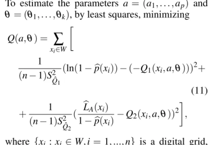
3. To estimate the parameters a= (a1, . . . ,ap) and

θ= (θ1, . . . ,θk), by least squares, minimizing

Q(a,θ) =

_∑

1

(n−1)S2_ˆ

Q₁

(ln(1−bp(xi))−(−Q1(xi,a,θ))) 2₊

(11)

+ 1

(n−1)S2_ˆ

Q₂

( bLA(xi)

1−_bp(xi)−Q2(xi,a,θ))

2

,

where {xi :xi ∈W,i=1, ...,n} is a digital grid,

b

Q1(x) =ln(1−pb(x)), Qb2(x) =bLA(x)/(1−bp(x))

andS2_ˆ

Q₁,S 2

ˆ

Q₂ are their respective sample variances.

In our applications, we have used well-known numerical methods to approximate the integrals (Eq. 10) and to minimize the function given in Eq. 11. In particular, the trapezoidal rule has been used to approximate the integrals (Eq. 10), and the fmincon function of the Matlab optimization toolbox has been used to solve the optimization

problem (Eq. 11). The purpose of fmincon is to

find a constrained minimum of a scalar function of several variables starting at an initial estimate. It uses a sequential quadratic programming method, solving a quadratic programming (QP) sub-problem at each iteration. At each iteration, an estimate of the Hessian of the Lagrangian is updated using the Broyden-Fletcher-Goldfarb-Shanno (BFGS) formula (Fletcher and Powell, 1963; Goldfarb, 1970); a line search is performed using a merit function similar to that proposed by Han (1977); Powell (1978a;b), and the QP subproblem is solved using an active

set strategy similar to that described in (Gill et al.,

1981). Researchers more expert than us in this field, will surely find numerical methods that provide better results, but our aim has simply been to show the method.

At this point we would like to point out that we are

just concerned with a particular type ofλ(x)functions,

whose functional form has been stated before. This type of intensity function is quite common in real

applications, although functions f and/or g could be

unknown. If f and/or g were unknown a reasonable

approximation could be considered; for example, f

could be modeled as a linear or exponential function

and g could be considered as a normal or uniform

density function.

In some cases, when the analytical expression

of functions Q1 and Q2 are known, the numerical

Example 1 Let us consider a particular case of NHBM (Def. 2) with λ(x) =a1+a2DROI(x), being

a= (a1,a2) constants to estimate. The radius of the

ball, r, is considered fixed but unknown, and the region of interest is a line. In this case:

Q1(x,a,r) =

Z

B(x,r)

a1+a2DROI(y)dy,

Q2(x,a,r) =

Z 2π

0

r(a1

+a2DROI(x−(rcos(θ),rsin(θ))))dθ,

and using the mean value theorem in both equations:

Q1(x,a,r) =πr2(a1+a2DROI(x)),

Q2(x,a,r) =2πr(a1+a2DROI(x)).

Thus it is not necessary to use any numerical

optimization algorithm to obtain ˆa₁,aˆ₂ and ˆr. Using

elemental calculus, similar to those used to obtain de minimum least squared line, the values of the parameters to minimize Eq. 11 will be:

ˆ

r=∆+ v u u t_∆2+4

S2_ˆ

Q₁

S2 ˆ Q₂

,

ˆ

a1=

ˆ

rS_DQˆ

1S

2 ˆ

Q₂+2SDQˆ2S

2 ˆ Q₁ π_br(rˆ2_S2

ˆ Q₂+4S

2 ˆ Q₁)S

2 D

,

ˆ

a₂=

S2_D(rˆQb₁S2_ˆ

Q₂+2Qb2)S 2

ˆ

Q₁−D(rSˆ DQˆ₁SQ2ˆ₂+2SDQˆ₂S2Qˆ₁) πrˆ(rˆ2S2_ˆ

Q₂+4S 2

ˆ Q₁)S

2 D

.

Being Qb₁ and Qb₂ the means of ln(1−pˆ(x)) and

ˆ

LA(x)/(1−pˆ(x)) respectively; D, and S2_D, the mean

and the variance of DROI(x); Sf g = (∑i(f(xi)−

¯

f)(g(xi)−g¯))/nand

∆=

S2

DQˆ₁S 2

ˆ Q₂−S

2 DQˆ₂S

2 ˆ Q₁+nS

2 D(Qb

2

1S2Qˆ₂−Qb 2

2S2Qˆ₁)

S2_ˆ

Q₂(SDQˆ₁SDQˆ₂+nS2DQb₁Qb₂)

.

SIMULATION STUDY

In this section, a simulation study is carried out to test the performance of the three estimation procedures explained previously.

Three different experiments are performed. For each one, 20 realizations of the particular non-homogeneous Boolean model introduced before are

simulated on a 512×512 window. Regarding the

model:

– The typical grain is assumed to be a ball, i.e.,

Ξ0=B(0,r).

– Two different intensity functions are considered:

λ(x) =a1+a2DROI(x)

and

λ(x) =a1exp{a2DROI(x)},

a1 and a2 being the parameters to estimate, and

DROI(x)the distance from pointxto the region of

interest.

– Two types of regions of interest, will also be

considered in each experiment: a line, and two different lines.

Fig. 1 shows realizations of some of

these particular NHBMs assuming that λ(x) =

0.01 exp{−0.05DROI(x)} and thatDROI(x) represents

the distance to a line (Fig. 1 (c)) and to two crossing lines (Fig. 1 (d)).

Results obtained using Molchanov’s, Schmitt’s and LSIVD methods will be compared.

Regarding our method:

– An Epanechnikov kernel with a bandwidth ofh=

70 has been used to estimate the area fraction function and the density of the boundary length (Eq. 8).

– As stated below, the trapezoidal rule has been used

to approximate Qi(x,a,θ),i=1,2 (Eq. 10), and

thefminconfunction of the Matlab optimization toolbox has been used to minimize the function stated in Eq. 11.

For smoothing purposes, in the method of Molchanov and Chiu (2000), the Epanechnikov kernel with a

bandwidthh of 70 has also been used to estimate the

area fraction function (Eq. 8).

To perform Schmitt’s method it is necessary to

choose a value for the tuning parameter ε, which

is related to the radius of the grain process. As the distribution of the radius is known in our simulations,

we will detail in each case, theε value used.

All the algorithms have been implemented in

Matlab1.

FIRST EXPERIMENT

In this first experiment we obtain 20 simulations

of a non-homogeneous Boolean model with

intensity function λ(x) = a+bD(x). Two different

combinations ofa,b and r values are considered for

image simulation: a = 1 e-5, b =2 e-5 (where e-5

denotes×10−5) and two differentr-values:r=5 and

r=10. To choose these values, it should be taken into

account that not every combination is valid. There will be combinations that could lead to images without any interest, for being either completely covered, or almost empty. For this reason they have been chosen ad hoc, after visualizing the simulated images. To perform

Schmitt’s method,ε =r+2 has been used.

Once obtained the images, parameters a, b and r

are estimated from them with the different methods exposed in the paper. Results of this first experiment can be found in Table 1.

SECOND EXPERIMENT

Let’s consider an exponential expression for the

intensity function,i.e.,λ(x) =aexp{−bDROI(x)}with

aandbbeing the constants to estimate. The radius of

the ball,r, is considered fixed but unknown.

Once again, parameters are chosen following the criteria explained in the first experiment. To perform

Schmitt’s method,ε =r+2 has been used.

The results are shown in Table 2.

THIRD EXPERIMENT

Let’s consider an exponential expression for the

intensity function, i.e., λ(x) = aexp{−bDROI(x)},

with a andb being the constants to estimate, and let

rfollow a uniform distribution on[0,R].

Once again, parameters are chosen in the same way as in the previous cases. To perform Schmitt’s method,

ε=R+2 has been used.

The results are shown in Table 3.

COMMENTS ON THE RESULTS

The main advantage of LSIVD method is its ability

to estimate r (or R), in addition to the parameters of

the intensity function, a and b, with a very simple

algorithm. As can be seen in Tables 1, 2 and 3, the three methods provide quite similar estimations, although subtle differences can be found between them. Molchanov’s method is the one that usually provides less accurate estimations, while LSIVD method is the one that usually presents the lowest variability in the estimations obtained. It is Schmitt’s

method that achieves the most accurate estimations in the highest number of cases.

It must also be noted that parameterr(respectively

R), is the parameter most efficiently estimated,

although it tends to be slightly overestimated.

Note that the performance of LSIVD method is usually somewhat worse than Schmitt’s, but Schmitt’s

method cannot estimate the value of r. Additionally,

in real applications the value of the tuning parameter

ε is unknown and its estimation could affect the

performance of the method. There is a modified version of Molchanov’s algorithm that makes it

possible to estimate rtogether with the parameters of

the intensity function, however, Molchanov provides a bit worse estimations than LSIVD method.

When analyzing the results, the difficulty of working with digital images should be kept in mind. For example, our circles are circles in a digital grid and it is therefore difficult to obtain a precise measure of their boundary length or their area. In our opinion, this may be causing the bias in the observed estimates. Our method could be improved with better digital measurements for the length of the curves and the area and with more accurate numerical methods for approaching the integrals and the optimization. In the

present study, the Matlab functionedgehas been used

to get the boundaries, and the number of pixels of these boundaries has been used to measure the lengths. The area has been also measured counting the number of pixels.

ANALYZING LONGLEAF PINES

DATA SET

spatstat(Baddeley and Turner, 2005) is a popular R-package for analyzing bidimensional point patterns, which includes some standard point pattern data sets. Among these standard data sets we can find the

Longleaf Pines data set (Platt et al., 1988; Rathbun

and Cressie, 1994), which is available as longleaf. The longleaf data set provides the location and diameters at breast height (dbh, a convenient measure of their size) of 584 Longleaf Pine (Pinus palustris) trees in

a 200 m×200 m region in southern Georgia (USA).

This data set represents a marked point pattern and it has been largely analyzed as an example of spatially

inhomogeneous point pattern (Baddeley et al., 2000;

Perry and Enright, 2006). Like Baddeleyet al.(2000)

and Perry and Enright (2006), we have considered only ‘adult’ trees, which are conventionally defined as those

with a dbh greater than or equal to 30 cm (Plattet al.,

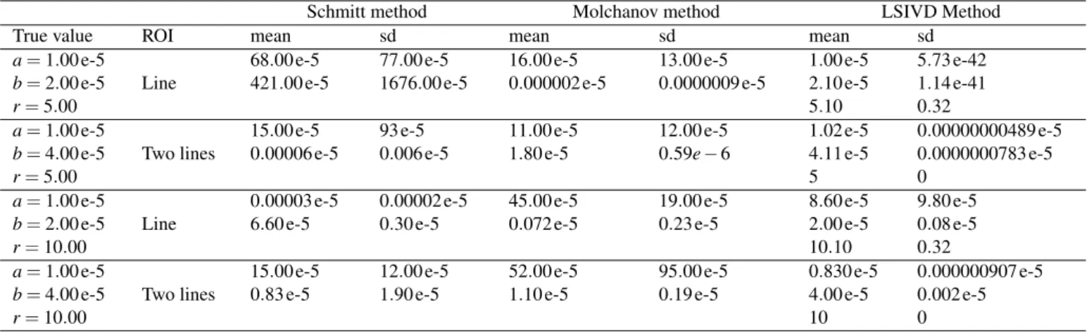
Table 1. Mean and standard deviation of the estimates of the parameters a, b, and r of the non-homogeneous Boolean model set in the first experiment.

Schmitt method Molchanov method LSIVD Method

True value ROI mean sd mean sd mean sd

a=1.00 e-5 68.00 e-5 77.00 e-5 16.00 e-5 13.00 e-5 1.00 e-5 5.73 e-42

b=2.00 e-5 Line 421.00 e-5 1676.00 e-5 0.000002 e-5 0.0000009 e-5 2.10 e-5 1.14 e-41

r=5.00 5.10 0.32

a=1.00 e-5 15.00 e-5 93 e-5 11.00 e-5 12.00 e-5 1.02 e-5 0.00000000489 e-5

b=4.00 e-5 Two lines 0.00006 e-5 0.006 e-5 1.80 e-5 0.59e−6 4.11 e-5 0.0000000783 e-5

r=5.00 5 0

a=1.00 e-5 0.00003 e-5 0.00002 e-5 45.00 e-5 19.00 e-5 8.60 e-5 9.80 e-5

b=2.00 e-5 Line 6.60 e-5 0.30 e-5 0.072 e-5 0.23 e-5 2.00 e-5 0.08 e-5

r=10.00 10.10 0.32

a=1.00 e-5 15.00 e-5 12.00 e-5 52.00 e-5 95.00 e-5 0.830 e-5 0.000000907 e-5

b=4.00 e-5 Two lines 0.83 e-5 1.90 e-5 1.10 e-5 0.19 e-5 4.00 e-5 0.002 e-5

r=10.00 10 0

Table 2. Mean and standard deviation of the estimates of the parameters a, b, and r of the non-homogeneous

Boolean model set in the second experiment.

Schmitt method Molchanov method LSIVD Method

True value ROI mean sd mean sd mean sd

a=1.00 e-2 1.02 e-2 1.55 e-2 0.40 e-2 0.05 e-2 0.53 e-2 0.04 e-2

b=5.00 e-2 Line 7.13 e-2 15.21 e-2 2.61 e-2 0.22 e-2 2.35 e-2 0.14 e-2

r=5.00 5.80 0.63

a=1.00 e-2 1.72 e-2 2.07 e-2 0.36 e-2 0.03 e-2 0.54 e-2 0.02 e-2

b=5.00 e-2 Two lines 8.69 e-2 18.41 e-2 1.98 e-2 0.21 e-2 2.18 e-2 0.05 e-2

r=5.00 5.80 0.63

a=1.00 e-2 1.05 e-2 1.10 e-2 0.25 e-2 0.07 e-2 0.48 e-2 0.53 e-2

b=5.00 e-2 Line 6.43 e-2 13.59 e-2 2.41 e-2 0.41 e-2 4.23 e-2 1.24 e-2

r=10.00 10.30 0.48

a=1.00 e-2 8.28 e-2 2.21 e-2 0.21 e-2 0.05 e-2 0.50 e-2 0.04 e-2

b=5.00 e-2 Two lines 5.85 e-2 1.69 e-2 1.60 e-2 0.47 e-2 4.74 e-2 0.83 e-2

r=10.00 10.10 0.31

From this data set we are going to use our method to estimate the parameters of the NHBM formed by the germ process of the locations of the trees and grain process of balls with a radius proportional to their respective diameters. It should be noted that it is not frequent to know the locations of trees in a forest because this is an expensive and hard task. Let us imagine that just an aerial photograph of this area was available for the study, then our sample information would be just a digital image showing the area covered by the trees. Assuming that the diameter of the crown of the tree is proportional to its diameter at breast height, the information available usually in this kind of problem is a binary image like the one shown in Fig. 4b.

Looking at Fig. 4b we can see that the area covered by trees is clearly growing from right to left in the region, so we can try to adjust the data to a non-homogeneous Boolean model assuming that the

intensity at a point x= (x1,x2), is a function of the

distance fromxto thex2-axis. An exponential function

is assumed,i.e.,λ(x) =aexp{−bD(x)}. With respect

to the radius distribution we are going to assume

the most simple one, a uniform distribution in[30,r].

Therefore, we have three parameters to estimate:a, b

andr.

Applying the method explained in section 4.3, the

estimates obtained are: ˆa=0.003, ˆb=−0.0062 and

ˆ

r=65.

longadult ● ● ● ● ● ● ● ● ● ● ● ● ●● ● ● ● ● ● ● ●●● ●● ● ● ● ● ● ●● ●●● ● ● ● ● ●● ●● ● ● ● ● ● ● ● ● ● ● ● ● ● ● ● ● ● ● ● ●● ● ● ● ● ● ● ● ● ●● ● ● ● ●● ● ● ● ● ● ● ● ● ● ● ● ●● ● ● ● ● ● ● ●● ● ● ● ●● ● ● ●● ● ● ● ● ● ● ● ● ● ● ● ● ●● ● ● ● ●● ● ● ● ● ● ● ● ● ● ● ● ● ● ● ● ● ● ● ● ● ● ● ● ● ● ● ● ● ● ●●●● ●● ● ● ● ● ● ● ● ● ● ● ● ● ● ● ● ● ● ● ●● ● ● ● ● ● ● ●●● ● ● ● ● ● ● ● ● ● ● ● ● ● ●● ● ● ● ● ● ● ● ● ● ● ● ● ● ●●● ● ● ● ● ●● ●●● ● ● ● ●●● ● ●● ● ●●● ● ● ● ● ●●●●● ● ● ● ● ● ● ● ● ● ● ● ● ● ● ● ● ● (a) (b)

Fig. 4. (a) Position of 271 adult pine trees in a

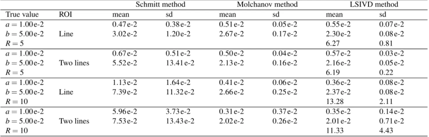
Table 3.Mean and standard deviation of the estimates of parameters a, b, and R of the non-homogeneous Boolean model set in the third experiment.

Schmitt method Molchanov method LSIVD method

True value ROI mean sd mean sd mean sd

a=1.00 e-2 0.47 e-2 0.38 e-2 0.51 e-2 0.05 e-2 0.55 e-2 0.07 e-2

b=5.00 e-2 Line 3.02 e-2 1.20 e-2 2.67 e-2 0.17 e-2 2.30 e-2 0.08 e-2

R=5 6.27 0.81

a=1.00 e-2 0.67 e-2 0.51 e-2 0.50 e-2 0.04 e-2 0.57 e-2 0.03 e-2

b=5.00 e-2 Two lines 5.52 e-2 13.41 e-2 2.13 e-2 0.16 e-2 2.16 e-2 0.05 e-2

R=5 6.19 0.22

a=1.00 e-2 1.13 e-2 1.64 e-2 0.41 e-2 0.06 e-2 0.36 e-2 0.08 e-2

b=5.00 e-2 Line 7.39 e-2 11.32 e-2 2.66 e-2 0.25 e-2 2.37 e-2 0.08 e-2

R=10 13.28 2.11

a=1.00 e-2 5.96 e-2 3.73 e-2 0.31 e-2 0.37 e-2 0.35 e-2 0.14 e-2

b=5.00 e-2 Two lines 7.53 e-2 13.43 e-2 2.02 e-2 0.26 e-2 2.01 e-2 0.71 e-2

R=10 11.33 4.43

We are going to use this “artificial” example to illustrate the performance of our proposed method. In this case, the germ point process locations are known (see Fig. 4a) and this allows us to estimate their intensity function using the point processes methods

implemented in the spatstat package. Therefore, we

can compare it with the one obtained using our method applied to Fig. 4b. This comparison can be seen in Fig. 5. The results are quite promising taking into account the difference in the information available in each case. Fig. 6 shows a couple of simulations of the fitted model for the image in Fig. 4b.

density.ppp(longadult, eps = 1)

0.002

0.004

0.006

0.008

0.01

0.012

(a) (b)

Fig. 5.(a) Estimated density function obtained using

point processes methods applied to Fig. 4a,b estimated density function obtained using our method applied to Fig. 4b.

Fig. 6.Simulations of the non-homogeneous Boolean

model fitted to the image of Fig. 4b.

GOODNESS OF FIT TEST

Once the parameters of the model have been estimated, it is necessary to check the adequacy of the model proposed, for modeling our data set. To this end, a Monte Carlo test of goodness of fit (Besag and Diggle, 1977; Diggle, 1983) is carried out.

We simulate 99 realizations of the model with the parameters estimated. In order to describe the

realizations, Kinhom, a generalization of the Ripley’s

K-function for second-order intensity-reweighted

stationary germ-grain models has been chosen

(Gallegoet al., 2014):

Kinhom(t) =

1

|W|E

Z

Ξ∩W

Z

Ξ∩B(y,t)

1

p(x)p(y)dydx

.

(12)

Let ˆKinhom0 and ˆKinhomi (i= 1,· · ·,99) be the

estimates of the K_inhom-function from the real image

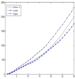
and the simulations. Fig. 7 shows the function

estimated from the real data, ˆKinhom0, and the lower

and upper envelopes of ˆKinhomi estimated from the

simulations. This indicates a satisfactory fit because ˆ

Kinhom0lies between the two envelopes except for a few

values.

Following Diggle (1983), we consider:

Di= Z t0

0

ˆ

Kinhomi(t)−K¯inhomi(t)

2

dt

1/2

,

i=0, ...,99,

where ¯Kinhomi=∑j6=iKˆinhomj/99.

Letr0 be the rank of D0. For r0>50 the Monte

Carlop-value is 2(100−r₀)/100. Meanwhile forr₀≤

50 it is 2(r0/100). The p-value obtained was 0.383,

Fig. 7.Lower and upper envelopes ofKˆinhomestimates

from the simulations and the estimated from the real data.

APPLICATION

In this section, we show how the NHBMs and our parameter estimation method can be applied to a phytopathological problem. As an illustration, we are going to analyze just one of the images obtained in an experimental study conducted by a group of researches from the Plant Physiology Section of Universitat Jaume I. The goal of their experimental study was to examine the robustness of callose deposition in response to different

pathogen-associated molecular patterns (Lunaet al., 2011). As a

result of the experiment, they obtained epifluorescence

microscopic images with a UV filter, of size 1536×

1920 pixels. As a preprocessing step, one of these colored images is selected and segmented into two binary images, one showing the nerves of the leaf and the other showing the callose deposition (Fig. 8). This second image shows small overlapping circular white spots. Mathematical morphological tools have been used to segment and convert the original image into binary images.

As can be seen in Fig. 8, callose deposition is mainly located close to the leaf nerves, presents a roughly circular shape and overlaps. That is why we propose to model their distribution with a non-homogeneous Boolean model, assuming that the

intensity at a pointx, is a negative exponential function

of the distance from x to the closest nerve or to the

edge of the leaf, i.e., λ(x) = aexp{−bD(x)}, with

D(X)defined as the minimum between the Euclidean

distance from a location x to its nearest nerve and to

the edge of the leaf. With this intensity function, there

will only be two parameters to estimate: a and b. If

we additionally assume that the grains are balls of a

fixed unknown radiusr, a third parameter must also be

estimated.

In the parameter estimation step, the algorithm previously detailed is followed. In order to estimate the area fraction (step 1) the Epanechnikov kernel is

used with band bandwidth h =80. In step 3, as in

our simulation study, the trapezoidal rule is used to

approximate the integral and the fmincon function

of the Matlab optimization toolbox has been used to solve the optimization problem.

The results obtained were ˆa=0.005, ˆb=1.5 and

ˆ

r=2 pixels.

(a) (b)

(c) (d)

Fig. 8.(a) Original image. (b) Binary image showing

the nerves of (a). (c) Callose deposition image of (a). (d) A simulation of the estimated model for the callose deposition image (c).

GOODNESS OF FIT TEST

Once we have estimated the parameters of the model, we need to check, once more, that this model that we assumed is appropriate for our data. For this purpose, we carry out again a Monte Carlo test of goodness of fit (Besag and Diggle, 1977; Diggle, 1983).

We simulate 99 realizations of the model with the parameters estimated. One of these simulations can be seen in Fig. 8d. In order to describe the realizations we have chosen a generalization of

the Ripley’s K-function for second-order

al., 2014).

Kinhom(t) =

1

|W|E

Z

Ξ∩W

Z

Ξ∩B(y,t)

1

p(x)p(y)dydx

.

(13)

Let ˆK_inhom0 and ˆK_inhomi (i =1,· · ·,99) be the

estimates of the Kinhom-function from the real image

and the simulations. Fig. 9 shows the function

estimated from the real data, ˆKinhom0, and the lower

and upper envelopes of ˆKinhomi estimated from the

simulations. This indicates a satisfactory fit because ˆ

K_inhom0lies between the two envelopes except for a few values.

Monte Carlo method is applied, getting a p-value

of 0.68, which leads us to accept the null hypothesis

formulated about the random distribution of callose deposition on leaves.

Fig. 9.Lower and upper envelopes ofKˆinhom estimates

from the simulations and the estimated from the real data.

CONCLUSIONS

In this paper we have proposed a simple statistical method that can be used to estimate the parameters of a particular kind of non-homogeneous Boolean model. In this model a particular functional form for the intensity function of the underlying process can be assumed. The method is based on applying least squared fitting to the area fraction function and the density of the boundary length. We have shown that it provides estimators as accurate as those obtained with other more complex methods for the general case. As an illustration, this model and the method have been used to analyze microscopical images from a phytopathological application. They can be used to

analyze images with similar characteristics in other scientific fields.

ACKNOWLEDGMENTS

We would like to thank Victor Flors from CAMN Department of the UJI for introducing us in this interesting problem and providing us the images. This work was supported by the Spanish Ministry of Economy and Competitiveness, project DPI2013-47279-C2-1-R and the Fundaci´o Caixa Castell´o

BANCAIXA, project P1.1A2011.11.

REFERENCES

Ayala G (1988). Inferencia en modelos Booleanos. Ph.D. thesis, Department of Statistics. University of Valencia. Baddeley A, Turner R (2005). Spatstat: an R package for analyzing spatial point patterns. J Stat Softw 12:1–42. Baddeley AJ, Møller J, Waagepetersen R (2000).

Non-and semi-parametric estimation of interaction in inhomogeneous point patterns. Stat Neerl 54:329–50. Berman M, Turner T (1992). Approximating point process

likelihoods with GLIM. J Roy Stat Soc C App 41:31–8. Besag J, Diggle P (1977). Simple Monte Carlo tests for

spatial pattern. J Roy Stat Soc C App 26:327–33. Bond J, Kofman L, Pogosyan D (1995). How filaments

of galaxies are woven into the cosmic web. Nature 380:603–6.

Bowman A, Azzalini A (1997). Applied smoothing techniques for data analysis: the kernel approach with S-Plus illustrations. Oxford University Press.

Brodatzki U, Mecke K (2001). Morphological model for colloidal suspensions. arXiv:cond.mat/0112009. Chiu S, Stoyan D, Kendall W, Mecke J (2013). Stochastic

Geometry and its applications. 3rd Ed. John Wiley & Sons.

Cressie N (1993). Statistics for spatial data. Wiley Series in Probability and mathematical statistics. New York: Wiley-Interscience.

Diggle P (1983). Statistical analysis of spatial point patterns. London: Academic Press.

Fletcher R, Powell M (1963). A rapidly convergent descent method for minimization. Comput J 6:163–8.

Gallego M, Ib´anez M, Sim´o A (2014). Inhomogeneous k-function for germ-grain models. arXiv:1401.8115 . Gill P, Murray W, Wright M (1981). Practical Optimization.

Academic Press.

Goldfarb D (1970). A family of variable metric updates derived by variational means. Math Comp 24:23–6. Han SP (1977). A globally convergent method for nonlinear

Hahn U, Micheletti A, Pohlink R, Stoyan D, Wendrock H (1999). Stereological analysis and modelling of gradient structures. J Microsc 195:113–24.

Luna E, Pastor V, Robert J, Flors V, Mauch-Mani B, Ton J (2011). Callose deposition: A multifaceted plant defense response. Mol Plant Microbe In 24:183–93. Lyman T (1972). Metals Handbook. American Society for

Metals.

Margalef R (1974). Ecolog´ıa. Barcelona: Omega.

Molchanov I (1997). Statistics of the Boolean model for practitioners and mathematicians. New York: J Wiley & Sons.

Molchanov I, Chiu S (2000). Smoothing techniques and estimation methods for nonstationary Boolean models with applications to coverage processes. Biometrika 87:265–83.

Molchanov I, Stoyan D (1994). Asymptotic properties of estimators for parameters of the Boolean model. Adv Appl Probab 26:301–23.

Perry G, Enright BMN (2006). A comparison of methods for the statistical analysis of spatial point patterns in plant ecology. Plant Ecol 187:59–82.

Platt W, Evans G, Rathbun S (1988). The population dynamics of a long-lived conifer (Pinus palustris). Am Nat 131:491–525.

Plaza M (1991). Contrastes en modelos germen y grano. Ph.D. thesis, University of Valencia.

Powell MJD (1978a). The convergence of variable metric methods for nonlinearly constrained optimization calculations. In: Mangasarian OL, Meyer RR, Robinson SM, eds., Nonlinear Programming 3. Academic Press. Powell MJD (1978b). A fast algorithm for nonlinearly

constrained optimization calculations. In: Watson GA, ed. Numerical Analysis. Lect Not Math 630:144–57. Quintanilla J, Torquato S (1997). Microstructure functions

for a model of statistically inhomogeneous random media. Phys Rev E 55:1558–65.

Rathbun S, Cressie N (1994). A space-time survival point process for a longleaf pine forest in southern Georgia. J Am Stat Assoc 89:1164–74.

Schmitt M (1996). Estimation of intensity and shape in a non-stationary Boolean model. In: Jeulin D, ed. Advances in theory and applications of random sets. Proc Int Symp.

Schneider R, Weil W (2008). Stochastic and integral geometry. Probability and its applications. Heidelberg: Springer-Verlag.

Serra J (1982). Image analysis and mathematical morphology. London: Academic Press. pp. 481–502. Weil W (2001). Densities of mixed volumes for Boolean