Design Optimization Average-Based Algorithm

(1)

Design Optimization Average-Based Algorithm

João Barradas Cardoso and Artur Barreiros

Department of Mechanical Engineering, Instituto Superior Técnico, University of Lisbon Av Rovisco Pais 1, 1049-001 Lisbon, Portugal

E-mail: [email protected], https://tecnico.ulisboa.pt/en/

Keywords: heuristic, randomness, population-based, optimization

Received: October 6, 2017

This article introduces a metaheuristic algorithm to solve engineering design optimization problems. The algorithm is based on the concept of diversity and independence that is aggregated in the average design of a population of designs containing information dispersed through a variety of points, and on the concept of intensification represented by the best design. The algorithm is population-based, where the population individual designs are randomly generated. The population can be normally or uniformly generated. The algorithm may start either with points randomly generated or with a designer preferred trial guess. The algorithm is validated using standard classical unconstrained and constrained engineering optimum design test problems reported in the literature. The results presented indicate that the proposed algorithm is a very simple alternative to solve this kind of problems. They compare well with the analytical solutions and/or the best results achieved so far. Two constrained problem analytical solutions not found in the literature are presented in annex.

Povzetek: Članek uvaja metahevristični algoritem za reševanje problemov optimizacije. Algoritem temelji na populaciji, kjer se naključno generirajo posamezni modeli posameznika in končno agregirajo v primerne rešitve.

1 Introduction

With the advent of fast, cheap and reliable computing power over the last decades, in addition to the application of classic optimization to larger and larger size problems, new alternative algorithms operating in a different fashion have been developed. The classical optimization algorithms have shortcomings and are not suitable for all optimization problems. The new alternative algorithms allow attacking optimization problems either too costly or not applicable to classical algorithms.

The purpose of heuristic algorithms applied to optimization problems is to search a solution to them by trial-and-error in a satisfying amount of computing time. The optimum solution is not guaranteed but a near optimum solution is accepted as a good solution. Metaheuristics refers to higher-level algorithms combining lower-level techniques and tactics for exploration and exploitation of the design space. That is, these algorithms, on one hand, must be able to generate a range of points in the whole design space including potentially optimum ones; on the other hand, they intensify the search around the neighborhood of an optimum or near optimum points (Yang, 2008).

Exploration and exploitation are the two important components of the metaheuristic algorithms. They are also called diversification and intensification (Glover, Laguna, 1997). A good balance of these components is required. Too much weight in diversification risks slow convergence with the solutions jumping around the potentially optimum ones; too much weight in intensification restricts the design space to a local region and risks the convergence to a local optimum (Blum,

Roli, 2003). The heuristic algorithms start typically either with guess solutions randomly generated or with a designer preferred trial solution. The diversification is gradually reduced as the algorithm proceeds; simultaneously, the intensification is increased.

One of the roles of injected randomness in stochastic search is to allow for movements to unexplored areas of the search space that may contain an unexpectedly good design. This is especially relevant when the search is stalled near a local solution. Injected randomness may also be used for the creation of simple random quantities that act like their deterministic counterparts, but which are much easier to obtain and more efficient to compute.

Metaheuristics algorithms are either population-based or trajectory-population-based. Examples of the former ones are the genetic algorithms (Holland, 1975) or the particle swarm optimization (Cagnina, Esquivel, Coello, 2008; Kayham, Ceylan, Ayvaz, Gurarslan, 2010) the last ones include the simulated annealing optimization (Kirkpatrick, Gelatt, Vecchi, 1983) or the harmonic search (Geem, Kim, Loganathan, 2001).

(2)

solvers, forecasters, and decision makers than any one individual. A classic example of group intelligence is the jelly-beans-in-the-jar experiment, in which invariably the group’s average estimate for the number of the jelly beans in the jar is superior to the vast majority of the individual guesses.

The theory that groups are remarkably intelligent and often smarter than the smartest people in them, demonstrates the significant impact on how businesses operate, how knowledge is increased, how economies are structured, and how people live their daily lives (Williams, 2006). The necessary conditions for a crowd to be wise include diversity, independence, and a specific type of decentralization. These conditions are essential to making good decisions which are the result of disagreement and contest rather than consensus or compromise.

Diversity means individuals have some private information or their own interpretation of known facts. Diversity helps because it actually adds perspectives that would otherwise be absent and because it takes away, or at least weakens, some of the destructive characteristics of group decision-making. Homogeneous groups are great at doing what they do well, but they become progressively less able to investigate alternatives. Independence means freedom from the influence of others. It keeps the individual mistakes from becoming correlated. Diversity is essential to preserving this independence. In the jelly-beans-in-the-jar experiment, most group members are not talking to each other or solving problems together.

Decentralization means people draw on local knowledge. It encourages individuals to make important decisions, not just in one location based only on one specific type of information, but dispersed through a variety of locations from where local knowledge is drawn and shared. The information coming out of a decentralized group must be aggregated throughout the system, to maintain a balance between local and global counterparts. Aggregation needs a mechanism that turns individual judgments into a collective decision. For instance, in a free market, the aggregating mechanism is price; in the jelly-beans-in-the-jar experiment, individual guesses were aggregated and then averaged, i.e., the aggregating mechanism is the average guess.

The aim of the present article is the proposal of an algorithm based on the concept just described. The algorithm considered is stochastic in the sense that it relies on random numbers and that different results may be obtained upon running the algorithm repeatedly. The algorithm is population-based, where the population individual designs are randomly generated. These individuals are diversified and independent since their design variables values are chosen stochastically without any correlation.

The individual designs are also decentralized since the design variables are chosen all over the entire design space. Finally, the different values of the design variables are aggregated as the plain or weighted average of those values. However, generating a diverse set of possible solutions isn’t enough. The designer, as the body of

people, also has to be able to distinguish the good solutions for the bad. So, at each of the iterations, the present algorithm selects two designs: the best design, the one with the best objective so far; and the averaged design, the one which design variable values are the mean of those variable values for the iteration.

The best design represents the intensification component of the algorithm; the averaged design represents the diversity part. In the current article, the optimization problem is understood as a minimization problem, where the function of merit to be assessed is an extended cost function that takes in account penalization due to violated constraints. A reference design is considered as a linear combination of both the best and the averaged design variables. A simple recurrence formula, centered on the reference design, is used to actualize the design for the next randomly generated population. The population can be normally or uniformly generated.

In optimization, there is traditionally a concern with developing a good stopping criterion. Unfortunately, the quest for an automatic means of stopping an algorithm with a guaranteed level of accuracy seems doomed to failure in general stochastic search problems. The fundamental reason is that in nontrivial problems, there will always be a significant region within the design space that will remain unexplored in any finite number of iterations, and there is always the possibility the optimum could lie in this unexplored region.

A danger arises in making broad claims about the performance of an algorithm based on the results of numerical studies. Performance can vary tremendously under even small changes in the form of the functions involved or the coefficient settings within the algorithms themselves. Outstanding performance on some types of functions is consistent with poor performance on other types of functions. This is a manifestation of no free lunch theorems (Spall, 2003; Wolpert, Macready, 1997).

The present algorithm is applied to several constrained and unconstrained test functions as well as to typical engineering design problems.

2 The optimal design problem

The optimal design problem may be formulated in a generalized fashion as

( )

0

min

. .

0; 1, 2,...,

; 1, 2,...,

j

il i iu

s t

j m

b b b i n



  =

  =

b b

b

(1)

where ₀is the cost or objective function, j are the constraints in a dimensionless form, b

(

b b₁, ₂,...,b_n

)

is the design vector, b_il and b_iu are respectively the lower and upper bounds of the design variable b_i.

(3)

0 0 0 b

min . .

; 1, 2,..., il i iu

P s t

b b b i n

   + 

  =

(2)

In Eq. (2), P stands for the penalty factor which value depends on the violation of the constraints as

1

0, for satisfied constraints

, for violated constraints m

P

m

 





=  

=  _ _





(3)

where





0

and m is the number of violated constraints. In practical terms, the constraint _j can be considered violated if  _j



, with  a very small number. Note that the absolute value of the objective is considered in the Eq. (2) in order to accommodate problems with negative objective functions.

3 The average concept algorithm

The present algorithm may be described by the flowchart of Fig. 1 as well as in the following manner:

1. Start with a preference design guess b and an imposed standard deviation, estimated as s_i=b_iu−b_il

(

i=1, 2,...,n

)

. Compute the starting values of ₀, j



(

j=1, 2,...,m

)

and 0, and establish the starting reference design bR as the preference guess, i.e. bR b.

Start iterates as

2. Launch a normally or uniformly random population of N designs as

k R k

i i i i

b =b +s r (4)

where i=1, 2,...,n, k=1, 2,...,N and r_ik is the k-th random number (with mean value 0 and standard deviation 1) related to the design variable b_i.

Do b_i=b_il if b_ib_il and b_i=b_iu if b_ib_iu.

3. Evaluate ₀, _j

(

j=1, 2,...,m

)

and ₀ for the entire population of N designs.

4. Evaluate the best design bB corresponding to the minimum value min0 of the extended function. Evaluate the averaged design bA for the distribution of designs as

1 1

N N

A k

k k

p p

= =

=



b b (5)

where bk is an arbitrary design vector in the population and p_k is the weight accounted for design

k

b on the average. The weights are selected by the designer. If a plain average is chosen, then pk =1 for

every design.

Another choice used in this work is to compare the

Evaluate the Best design and the Averaged design Compute starting objective,

Constraints and Extended objective

END Optimum design Optimum objective Constraint violation? Objective improvement?

it = it + 1 Starting design Starting standard deviation

Iteration (it) = 0

Launch a random population of designs

Compute current objectives, Constraints and Extended

objectives Evaluate the Reference design

by linear combination best and averaged design

N Y

Figure 1: Flowchart of the algorithm.

θ Starting Point

(-2.5, -2.5) (-2.5, 2.5) (2.5, -2.5) (2.5, 2.5) 1.00

(0.08986,-0.71283) -1.0316283 at iteration 38

(0.09140,-0.71266) -1.0316191 at iteration 39

(-0.09162,0.71276) -1.0316163 at iteration 36

(0.08887,-0.71247) -1.0316248 at iteration 31 0.85

(0.08979,-0.71267) -1.0316285 at iteration 15

(0.08997,-0.71265) -1.0316285 at iteration 21

(-0.08991,0.71265) -1.0316285 at iteration 21

(-0.08976,0.71272) -1.0316285 at iteration 15 0.25

(0.08973,-0.71262) -1.0316285 at iteration 36

(-0.08992,-0.71259) -1.0316285 at iteration 29

(0.08974,-0.71262) -1.0316285 at iteration 26

(-0.08973,0.71262) -1.0316285 at iteration 37 0.00

(0.09002,-0.71401) -1.0316136 at iteration 989

(-0.09020,0.71196) -1.0316237 at iteration 617

(0.09020,-0.71196) -1.0316237 at iteration 617

(4)

values of the extended function 0 and of the best extended function min0 in the previous iteration; and

then assign a weight p_k =2 if the first value is smaller than the second one, and a weight pk =1 if it

is equal or larger.

5. If there are no constraint violations and there are no improvements of the objective function within a prescribed number of iterations, go to 7.

6. Evaluate a reference design as the linear combination

(

1

)

R = B+ − A

b b b (6)

with

0  



1

and assume the distribution of designs k

b centered at bR with a standard deviation vector evaluated as _s=2_bA−_bB _.

Go to 2. End the iterates. 7. Stop.

In order of handling tabular discrete value design variables, the Eq. (4) is rewritten in these cases as

int

R k

k i i i

i

b s r

b = _ + _



  (7)

where  is the difference value between two consecutive design variables.

4 Numerical applications

In this Section one is going to solve unconstrained as well as constrained optimization problems by applying the formulation and the algorithm presented on the previous sections. With respect to the unconstrained problems, the applications are the minimizations of the benchmark following test functions: Six-Hump Camelback function, Rosenbrock and Michalewicz’s functions.

Concerning to the constrained problems, one solves three well-known engineering design optimization test problems: the welded beam design, the pressure vessel design and the tension-compression spring design. For all the applications normally distributed populations were used. A total of 30 independent runs were performed per problem. In the Sections 4.1 to 4.6 the runs of the algorithm were performed with a particular initial seed for different population sizes and different weights on the calculation of the average and reference designs.

The results are compared with analytical solutions and/or heuristic and nonlinear programming algorithms.

4.1 Six-Hump Camelback function

This function is one of the typical test functions in unconstrained global optimization (Dixon, Szego, 1975; Lee, Geem, 2005). It is mathematically expressed as

2 4 6 2 4

0 1 1 1 1 2 2 2

1

4 2.1 4 4

3

x x x x x x x

 = − + + − + (8)

Within the bounded region, this function has six local minima. Two of them are global minima located at either

(

−0.08984, 0.71266

)

or

(

0.08984, 0.71266−

)

, each with the corresponding function value equal to

0 1.0316285 

 = − .

For the algorithm presented here, a population of size

N

=

20

and a plain average in the step 4 were used within the design space −2.5x x₁, ₂2.5. For different values of the θ-factor and two starting points, the Table 1 gives the corresponding achieved solutions and the number of iterations needed for convergence.

We should note that the best and fastest solutions are obtained with



=

0.85

, i.e., giving respectively at each iteration, the weights 0.85 and 0.15 to the best and average points of the prior iteration in the formation of the current reference design.

With the starting point

(

2.5, 2.5

)

, corresponding to the cost value  =₀ 161.8489685, and with



=

0.85

, the present algorithm achieves the minimum cost value

0 1.0316285 

 = − at the point

(

−0.08976, 0.71272

)

after 15 iterations. However, after 9 iterations, the algorithm gets the cost value  = −₀ 1.0316285 at the point

(

−0.08799, 0.71382

)

, not far off the analytical solution. We should also note that the worst results exist for

0 

=

, i.e., only considering the average design as the design of reference. For



(

2.5, 2.5

)

and the weighted average (second) option on step 4 described in Chapter 3 instead of the plain average, the global optimum 0 1.0316285



 = − is obtained at the point

(

−0.08988, 0.71266

)

after 19 iterations.

Better results can be expectedly obtained by increasing the population size. For

N

=

(

2.5, 2.5−

)

, corresponding both to the minimum function value  = −₀ 1.0316285. For

N IP Iterate x1 x2 0

1000 0 4 -0.0897507 0.7126449 -1.0316285 1 5 -0.0898749 0.7127146 -1.0316285 100 0 13 -0.0897433 0.7126887 -1.0316285 1 11 -0.0898545 0.7126102 -1.0316285 20 0 15 -0.0897623 0.7127175 -1.0316285 1 19 -0.0898786 0.7126648 -1.0316285 Table 2: Camelback’s optimal solutions for



=

0.85

(5)

1000

N

=

and



=

0.85

, and starting from the point

(

−2.5,−2.5

)

, the optimum solution x =

(

0.08975, 0.71264−

)

,  = −₀ 1.0316285 has been achieved after 4 iterations.

Table 2 shows the optimal solutions achieved for different N population sizes and different average choices on Eq. (5),

IP

=

0

standing for plain average and

1

IP= _{meaning weighted average as written on step 4 of} the algorithm described on Chapter 3, using



=

0.85

and with the starting point located at

(

2.5, 2.5

)

.

We may note that is the population size

N

=

20

numerical solution, however, poses a particular challenge. The solution lies inside a very deep, narrow, banana shaped valley. The valley causes a lot of troubling for nonlinear programming search algorithms.

Using a population of 1000 samples within the design space −10.0x x₁, ₂10.0, a plain average, the factor



=

)

2 ₂₀

2 0

1

sin i sin i i

x i x 

=

 

 = −



_ _ (10)

with 0x x₁, ₂



.

The function is tricky; it has several local minimum values and several flat areas which make the one global minimum value hard to find numerically. Its global minimum is 0 1.8012980



 = − at the point

₌

x

(

2.20319, 1.57049

)

.

Using a population with size

N

=

20

samples within the design space 0.0x x₁, ₂4.0, a plain average, the factor



=

0.85

, and a starting point x=

(

2.0, 2.0

)

corresponding to  = −₀ 0.3701513, the present algorithm achieves the optimum point

(

2.20281, 1.57079

)

₌

x and the corresponding cost value  = −₀ 1.8013037 after 24 iterations. However, after 13 iterations the algorithm achieves the point

(

2.20258, 1.56925

)

=

x corresponding to the objective value  = −₀ 1.8012055. Changing the population size to

100 N

=

, the global minimum  = −₀ 1.8013039 is achieved after 10 iterations at the point

(

2.20289, 1.57091

)

₌

x . Changing now the population size to

N

=

1000

, the global minimum

0 1.8013039



 = − is achieved after 8 iterations at the point x=

(

2.20292, 1.57076

)

. The smallest number of function evaluations

(

20 24

)

is obtained for

N

=

20

.

4.4 Welded beam design

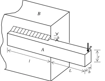
The welded beam design problem is well studied in the context of single-objective optimization. A beam A needs to be welded on another beam B and must carry a certain load P as shown in Fig. 2. The welded beam is designed for minimum fabrication cost subject to constraints on

t h

P

b l

L

A B

(6)

shear stress τ, bending stress in the beam σ, buckling load on the bar P_c, end deflection of the beam δ, cost of the weld and beam A materials, and side constraints (Ragsdell, Phillips, 1975; Rao, 1996). One wants to find four design parameters: thickness of the beam b, width of the beam t, length of the weld l, and thickness of the weld h.

)

(

)

2

0 1 2 1 2 3 3 4 2

1 max

2 max

3 1 4

2

4 1 1 3 3 4 2

5 max

6

1

4

1 2

min

. .

1 0 1 0 1 0

5 1 0

1 0

0.125 2

0.1 2

0.1 , 10

c

C C x x C x x L x

s t

x x

C x C x x L x

P P x x x x

   

 

  + + +

  − 

 

 _ + + _ − 

  − 

 

(11)

where 3

1 0.10471 $ / in

C = is the cost per unit volume of

the weld material, C₂=1 $ / in3 is the labor cost per unit weld volume, C₃ =0.04811 $ / in3 is the cost per unit volume of the beam B,



)

,

2 M R J



= , M =P L

(

+x₂ 2

)

,

(

)

2 2

2 1 3

0.5

R= x + x +x ,

(

3

)

3 4

6P L x x

 = ,

(

)

3 3

3 4

4P L E x x

 = ,

(

)

2

(

)

2

1 2 2 1 3

2 6 3

J= x x _x + x +x _,

(

2

)(

3

)

(

)

3 4 3

4.013 6 1 0.5 0.25

c

P = E L x x _ − x L E G_,

6

30 10 psi

E=  , G=12 10 psi 6 , P=6, 000 lb,

14 in L=

By using mathematical programming, (Rao, 1996) presents the optimum cost function  =₀ 2.3810

corresponding to the design point x =

(

0.2444, 6.2177, 8.2915, 0.2444

)

. A better nonlinear programming solution has been achieved in (Andrei, 2013) by adding GAMS created nonlinear model:

0 1.72485 

 = , x =

(

0.206, 3.470, 9.037, 0.206

)

. The lowest optimal solution known so far by the

N IP Iterate x1 x2 x3 x4 0

5000 0

16645 0.205729 3.470519 9.036630 0.205730 1.724858 268 0.205468 3.476687 9.038588 0.205723 1.725573 32 0.205436 3.477702 9.034963 0.205964 1.726863 16 0.204191 3.530001 9.042473 0.205769 1.731815 1

11144 0.205726 3.470586 9.036639 0.205730 1.724864 303 0.204957 3.488440 9.035478 0.205797 1.726386 57 0.205409 3.475931 9.042488 0.205808 1.726697 19 0.204431 3.523721 9.041501 0.205707 1.730704

1000 0

9434 0.205727 3.470567 9.036656 0.205730 1.724866 27 0.204332 3.495317 9.051999 0.205779 1.729056 19 0.204359 3.503654 9.084193 0.205596 1.734414

1

10419 0.205730 3.470530 9.036634 0.205730 1.724866 1335 0.205707 3.470647 9.038382 0.205760 1.725373 522 0.205451 3.477778 9.038218 0.205742 1.725777 37 0.205635 3.479632 9.039730 0.205804 1.727052 21 0.206227 3.492924 9.013144 0.206816 1.732874

100 0

15080 0.205727 3.470617 9.036695 0.205729 1.724877 1596 0.205693 3.470650 9.039433 0.205731 1.725315 205 0.205585 3.477111 9.031481 0.206261 1.728674 177 0.206150 3.503281 9.041299 0.206170 1.734152 1

27689 0.205724 3.470646 9.036589 0.205731 1.724869 672 0.204555 3.495600 9.037673 0.205735 1.726630 300 0.205584 3.488843 9.039643 0.205969 1.729467 141 0.202780 3.547630 9.027128 0.206246 1.732925

20 0

11462 0.205731 3.470480 9.036694 0.205735 1.724909 2265 0.205546 3.475157 9.036914 0.205765 1.725515 714 0.207129 3.459350 8.988936 0.208278 1.736547 1

22011 0.205726 3.470606 9.036623 0.205730 1.724868 2788 0.205607 3.474374 9.036784 0.205731 1.725223 115 0.202686 3.587231 9.037897 0.205726 1.736020

(7)

authors is given in (Kayham, Ceylan, Ayvaz, Gurarslan, 2010): x =

(

0.205830, 3.468338, 9.036624, 0.205730

)

and  =₀ 1.724717.

The optimization results achieved with the present algorithm are shown in Table 3 for different population sizes N and different average choices on Eq. (5). The first row for each choice combination of N and IP represents the optimum at the convergence of the algorithm. The following rows are the results at intermediary iterations. For all these design points all the constraints are satisfied.

The best minimum cost value obtained in the present article is  =₀ 1.724858, corresponding to the point

(

0.205729, 3.470519, 9.036630, 0.205730

)

 ₌

x .

One may observe that the algorithm solutions compare very well with the best solution presented above, even for earlier iterates of the algorithm. We may also observe that convergence is faster when the plain average is used in Eq. (5).

4.5 Pressure vessel design

The pressure vessel design problem has been proposed in (Kannan, Kramer, 1994). It is one of the most used test problems for validating optimization algorithms. The problem is to find the optimal design of a compressed air storage tank (Fig. 3) with a working pressure of 1000 psi and a minimum capacity volume of V_min =1, 296, 000in3.

The pressure vessel is composed of a cylindrical shell capped at both ends by hemispherical heads.

Let the design variables be x₁T_s the thickness of the shell, x₂T_h the thickness of the heads, x₃R the inner radius and x₄L the length of the cylindrical shell. The variables x₁ and x₂ should be integer multiples of 0.0625 in. The objective is to minimize the manufacturing cost (material, welding and forming costs) of the pressure vessel (Sandgren, 1990), subjected to constraints on volume capacity and in accordance with

respective ASME codes. The mathematical model of the problem is:

(

)

2

0 1 3 4 2 3

2 2

1 4 1 3

1 3 1

2 3 2

3 min

2 3

3 4 3

1 2

3 4

min 0.6224 1.7781

3.1661 19.84 . .

0.0193 1 0

0.00954 1 0

1 0

4 3

0.0625 , 99 0.0625

10 , 200

x x x x x

x x x x

s t

x x x x V V

V x x x

x x x x



  + +

+

  − 

= +

  

 

(12)

The analytical optimum for this problem is calculated in the Annex A as  =₀ 6059.714335 at

(

)

*

0.8125, 0.4375, 42.0984456, 176.6365958 =

x with

the first and third constraints being active.

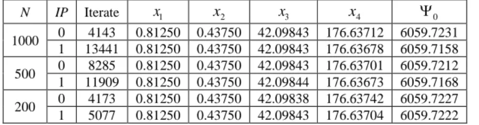
The optimal results achieved with the present algorithm are shown in Table 4 for different population sizes N and different average choices on Eq. (5). For all these solutions there is no violation of the constraints. The first constraint is nearly active at the optimal point for all the different population sizes; it takes values in the interval −0.3666 10 −7    −₁ 0.1215 10 −5.

The results for the present algorithm compare well with the analytical solution. Again, the plain average of the Eq. (5) gives origin to faster convergence.

4.6 Tension/Compression spring design

The tension/compression spring design optimization problem is described in (Arora, 1989). The goal is to minimize the weight of a tension/compression spring (Fig. 4) subject to constraints on minimum deflection, shear stress, surge frequency, limits on outside diameter and side constraints. The design variables to be considered are the wire diameter d, the mean coil diameter D and the number n of active coils.

Let us set up the vector of design variables as

(

x x x1, 2, 3

)



x 

(

d D n, ,

)

.

L

R R

Th Ts

Figure 3: Pressure vessel.

N IP Iterate x₁ x₂ x₃ x₄ ₀

1000 0 4143 0.81250 0.43750 42.09843 176.63712 6059.7231 1 13441 0.81250 0.43750 42.09843 176.63678 6059.7158 500 0 8285 0.81250 0.43750 42.09843 176.63701 6059.7212 1 11909 0.81250 0.43750 42.09844 176.63673 6059.7168 200 0 4173 0.81250 0.43750 42.09838 176.63742 6059.7227 1 5077 0.81250 0.43750 42.09843 176.63704 6059.7222

Table 4: Pressure vessel optimal solutions.

d

D

P P

(8)

The problem may be formulated as

(

)

(

)

(

)

(

)

(

)

(

)

(

)

2

0 3 1 2

3 4

1 2 3 1

2 3 4

2 2 1 2 2 1 1

2 1

2

3 1 2 3

4 1 2

1

2

3

min 2

. .

1 71785 0

4 12566

1 5108 1 0

1 140.45 0

1.5 1 0

0.05 2 0.25 1.3

2 15

x x x

s t

x x x

x x x x x x

x

x x x

x x

x x x

  +

  − 

 

  − _ − _+

− 

  − 

  + − 

 

(13)

The analytical solution for this problem is presented in the Annex B. The minimum weight of the spring is achieved as  =₀ 0.012665232 at the point

(

)

*

0.051690, 0.356740, 11.287642 =

x . At the optimum,

the constraints ₁ and ₂ are active, and

3 4.054 

 = − ,  = −₄ 0.7277.

The minimum objective function value obtained in (Arora, 1989) by nonlinear programming is

0 0.012679 

 = corresponding to the optimum point

(

0.051699, 0.35695, 11.289

)

x = . The best result known

so far by the authors is given in (Cagnina, Esquivel, Coello, 2008) as  =₀ 0.012665, with

(

)

*= _{0.051583, 0.354190, 11.438675}

x .

The optimum results achieved with the present algorithm are shown in Table 5, for

IP

=

0

, different sizes N of the population and plain average selection on Eq. (5). For all these solutions there is no violation of the constraints, being practically active the first two constraints ₁ and ₂. The last two constraints have values within the intervals −4.08   −₃ 4.04 and

4

0.734  0.720

−    − .

Again, the present algorithm results compare well with the analytical solution.

5 Concluding remarks

This article presents an average concept algorithm to solve various optimization problems which include typical benchmark functions unconstrained problems and structural engineering test design constrained problems.

To evaluate the performance of the present algorithm, numerical applications are conducted and the results are compared to the results obtained analytically and/or to the best ones achieved by other optimization methods. The analytical solutions for two of the constrained problems, namely the pressure vessel design and the tension-compression spring design problems, are determined in the present article. The solutions found by the proposed algorithm compare well with those results.

We may conclude that the algorithm finds the global solution or a near-global solution in each problem tested. The Six-Hump Camelback function, for example, has 6 local minimal points; however, the algorithm converges to the global minima.

Characterizing the principal advantage of the algorithm one should emphasize the good balance between the accuracy of the solutions it achieves and its rare simplicity.

References

[1] Andrei, N. (2013) Nonlinear Optimization Applications Using the GAMS Technology. Springer Science & Business Media.

https://doi.org/10.1007/978-1-4614-6797-7

[2] Arora, J. S. (1989) Introduction to Optimum Design. McGraw-Hill, New York.

https://doi.org/10.1016/C2013-0-15344-5

[3] Blum, C., Roli, A. (2003) Metaheuristics in Combinatorial Optimization: overview and conceptual comparison. ACM Computing Surveys. 35, 268-308.

https://dl.acm.org/doi/pdf/10.1145/937503.937505 [4] Cagnina, L.C., Esquivel, S.C., Coello, C.A.C.

(2008) Solving Engineering Optimization Problems with the Simple Constrained Particle Swarm Optimizer, Informatica. 32, 319-326.

[5] Dixon, L.C.W., Szego, G.P. (1975) Towards Global Optimization. North Holland.

[6] Geem, Z.W., Kim, G.H., Loganathan, G.V. (2001) A New Heuristic Optimization Algorithm: Harmonic Search. Simulation. 76, 60-68.

https://doi.org/10.1177/003754970107600201 [7] Glover, F., Laguna, M. (1997) Tabu Search. Kluwer

Academic Publishers.

https://doi.org/10.1007/978-1-4613-0303-9_33 [8] Holland, J.H. (1975) Adaptation in Natural and

Artificial Systems. The University of Michigan Press: Ann Arbor.

[9] Kannan, B.K., Kramer, S.N. (1994) An Augmented Lagrange Multiplier Based Method for Mixed Integer Discrete Continuous Optimization and its Applications to Mechanical Design. Journal of Mechanical Design. 116, 318-320.

https://doi.org/10.1115/1.2919393

[10] Kayham, A.H., Ceylan, H., Ayvaz, M.T., Gurarslan, G. (2010) PSOLVER: A New Hybrid Particle Swarm Optimization Algorithm for Solving Continuous Optimization Problems. Expert Systems with Applications. 37, 6798-6808.

https://doi.org/10.1016/j.eswa.2010.03.046

N 1000 500 200 100

0

 0.012665 0.012666 0.012668 0.012671

1

x 0.051718 0.051775 0.051308 0.052127 2

x 0.357409 0.358778 0.347629 0.367321

3

x 11.248693 11.169669 11.842695 10.694988

Iterate 10063 11690 24818 13899

(9)

[11] Kirkpatrick, S., Gelatt, C.D., Vecchi, M.P. (1983) Optimization by Simulated Annealing. Science. 220, 671-680.

https://doi.org/10.1126/science.220.4598.671 [12] Lee, K.S., Geem, Z.W. (2005) A New

Meta-Heuristic Algorithm for Continuous Engineering Optimization: Harmony Search Theory and Practice. Computer Methods in Applied Mechanical Engineering. 194, 3902–3933.

https://doi.org/10.1016/j.cma.2004.09.007

[13] Luenberger, D.G. (1984) Introduction to Linear and Nonlinear Programming. Addison-Wesley, Massachusetts.

https://doi.org/10.1007/978-0-387-74503-9

[14] Moré, J.J., Garbow, B.S., Hillstrom, K.E. (1981) Testing Unconstrained Optimization Software. ACM Transactions on Mathematical Software. 7, (1), 17- 41.

https://doi.org/10.1145/355934.355936

[15] Papalambros, P.Y., Wilde, D.J. (1988) Principles of Optimal Design: modeling and computation. Cambridge University Press, New York.

https://doi.org/10.1017/9781316451038

[16] Ragsdell, K. M., Phillips, D.T. (1975) Optimal Design of a Class of Welded Structures Using Geometric Programming. ASME J. Eng. Ind. Ser. B. 98 (3), 1021–1025.

https://doi.org/10.1115/1.3438995

[17] Rao, S.S. (1996) Engineering Optimization Theory: and Practice. John Wiley & Sons.

https://doi.org/10.1002/9780470549124

[18] Rosenbrock, H.H. (1960) An Automatic Method for Finding the Greatest or Least Value of a Function. Computer Journal. 3, 175-184.

https://doi.org/10.1093/comjnl/3.3.175

[19] Sandgren, E. (1990) Nonlinear Integer and Discrete Programming in Mechanical Design Optimization. Journal of Mechanical Design. 112 (2), 223–229. https://doi.org/10.1115/1.2912596

[20] Spall, J.C. (2003) Introduction to Stochastic Search and Optimization: estimation, simulation and control. John Wiley&Sons.

https://doi.org/10.1002/0471722138

[21] Surowiecki, J. (2005) The Wisdom of Crowds: Why the Many Are Smarter Than the Few and How Collective Wisdom Shapes Business, Economies, Societies and Nations. Anchor Books.

[22] Williams, S. (2006) The Wisdom of Crowds: why the many are smarter than the few and how collective wisdom shapes business, economies, societies, and nations. Business Book Review™. 21 (43).

[23] Wolpert, D.H., Macready, W.G. (1997) No Free Lunch Theorems for Optimization. IEEE Transactions on Evolutionary Computation. 1, 67-82.

https://doi.org/10.1109/4235.585893

[24] Yang, X.S. (2008) Nature-inspired Metaheuristic Algorithms. Luniver Press.

Annex A: Pressure Vessel Classical

Design Optimization

Let us assume initially the variables x1_and x2_are

continuous and later on make the convenient correction to table (multiple of 0.0675) values.

The cost function 0_{decreases monotonically with} 1

x _or x₂_{decrease. The constraint} ₁_{is the only}

constraint that increases as x1_{decreases, and the}

constraint 2_{is the only constraint that increases as}x2

decreases. Then, 1_and2_{provide respectively lower}

bounds for x1_and x2_{, and these variables may be}

minimized out as

1 3

2 3

0.0193 0.00954

x x

=   =

 (A1)

Substituting these relationships into the original problem, we have

( )

2 3

0 3 4 3

2 3

3 3 4 3

3 4

min 0.01319166 0.024353275 . .

1296000 4 3 0

10 , 200

x x x

s t

x x x

x x

 

  +

  − − 

 

(A2)

where the upper bars on the cost and constraint symbols mean we are determining by now the solution for all variables continuous. The Lagrangian function for this problem is

(

)

(

)

(

)

(

)

0 3 3 3 3 3 3

4 4 4 4

10 200

L x x

x x

  

 

− +

=  +  − − + − −

− + − (A3)

where



₃, ₃−, ₃+, ₄−, ₄+ are the Lagrange multipliers for the constraint ₃ and side constraints. The necessary Karush-Kuhn-Tucker conditions (Arora, 1989) for the problem (A.2) may now be set as

(

)

( )

(

)

(

)

2

3 3 4 3

2

3 3 4 3 3 3

2 2

4 3 3 3 4 4

2 3

3 3 3 3 4 3

3 3 3 4 4

2

3 3 4

2 0.01319166 3 0.024353275

2 2 0

0.01319166 0

1296000 4 3 0

10 0, 200 0, 3, 4

, , , , 0

1296000 4

k k k k

L x x x x

x x x

L x x x

x x x

x x k

x x

   

   

 

     

− +

− + − +

    + 

− + − + =

   − − + =

 

  _ − − _=

− = − = =



  − −

( )

3

3 4

3 0

10 , 200

x x x

 

 

(10)

Let us now search the different combinations of Lagrange multipliers:

1. ₃−0, ₄−0 

3 4 10, 3 1288669.6

x =x =  = (violated)

3 0, 4 0

−_ + _ _

3 10, 4 200, 3 1228979.4

x = x =  = (violated)

Then, whatever the value of



₃, must have ₃− =0

2.



₃=0

2.1 ₃− =0  3 0

+ _ _{(from the 1}st_{condition, then} violating the 5th_one)

2.2 ₄−=0  ₄+ 0 (from the 2nd_{condition, then} violating the 5th_one)

3. ₃0  =₃ 0 

( )

2

( )

4 1296000 3 4 3 3

x = x − x

3.1 ₃+ =₄− =₄+=0 



₃=0.01319166



(from the 2nd_{condition) and}

3 0

x = (after substituting x₄ and



₄ into the 1st_one) 3.2 ₃+ =₄−=0, ₄+0  x4=200 (from the 4

th

condition),

( )

2 3

3 4 3

1296000−x x − 4 3 x =0 

3 40.3196187244

x =

(

)

2

3 4 3

3 2

3 4 3

2 0.01319166 + 3 0.024353275

2 2

0 004663057579 0

x x x

.     = + =  2 2

4 3 3 0 01319166 3

2 369851195 0

x . x

.

+₌  ₋

= 

All the optimality necessary conditions are satisfied, then 1 3 2 3 3 4 0.0193 0.778168646 0.00954 0.384649165 40.3196187244 200 x x x x x x = =   = =   =   = 

is candidate local optimum point for the assumed continuous variables.

3.3 ₃+=₄+ =0, ₄−0  x₄=10 (from the 4th condition),

( )

2 3

3 4 3

1296000−x x − 4 3 x =0 

3 65.2252326139

x =

(

)

2

3 4 3

3 2

3 4 3

2 0.01319166 + 3 0.024353275

2 2

x x x





 

=

+

0 005698937505. 0

= 

2 2

4 0 01319166 3 3 3

20 04674872 0

. x x

.

−₌ ₋ 

= − 

(violates 5th_condition)

3.4 ₄− =₄+ =0, ₃+0 x3=200  4 256.3534264 0

x = − 

3.5 ₄−=0, ₃+ 0, ₄+ 0  x₃=x₄=200

3 57347062.87 0

 = − 

(contradicts point 3:  =₃ 0)

3.6 ₄+=0, ₃+ 0, ₄− 0 x3=200, x4=10   = −₃ 33470958.70

(contradicts point 3:  =₃ 0)

Testing now the second-order sufficient conditions for the only point x( ,x x x x₁ ₂, , )₃ ₄ , determined in 3.3, satisfying the necessary conditions, one may use the so-called bordered Hessian (Luenberger, 1984) calculated at that point:

(

)

2 3 23 2 3 4

3 3 3 3 3 3 4

2 2 2

3 4 3 4 4

0 ,

0 71095.91969 5107.198124 71095.91969 232.2341915 0.117553254 5107.198124 0.117553254 0

x x

x x x L x L x x

x L x x L x

          _      _           − −     = −_ − _ − −    B

As n m− for the problem (A.2) is 2 1− =1 one has to calculate the last principal minor det

( )

B . Since its value is negative, its sign is coincident with

( )

1m

( )

1

sign − =sign − . Hence, the Hessian of L is positive-definite and the point

x

is a minimum point.

Now, rounding up the values of x₁ and x₂ to the table values, we have

1 2 0.8125 0.4375 x x    =   = 

then determine the other two variables as





3 min 0.8125 0.0193, 0.4375 0.00954

42.0984456 x =

=

From the two first constraints x₃0.8125 0.0193,

3 0.4375 0.00954

x  , i.e., the constraint ₁ is active at the optimum, and

4 176.6365958

x=

from the condition of  =₃ 0 

( )

2

( )

4 1296000 3 4 3 3

x = x − x

Therefore, the analytical optimum point for the pressure vessel design problem is

(

0.8125, 0.4375, 42.0984456, 176.6365958

)

(11)

giving the minimum optimum cost  =₀ 6059.714335. At the optimum, the constraints have  =  =₁ ₃ 0 and

2 0.082013323 

 = − .

Annex B: Tension-Compression

Spring Classical Design Optimization

Again, let us firstly to analyze the monotonicity of the problem (Papalambros, Wilde, 1988). One should observe the constraint ₁ is critical with respect to the design variable x₃. The cost function ₀ increases monotonically in the variable x₃, and there is exactly one constraint, the constraint ₁, whose monotonicity with respect to x₃ is opposite from that of the objective. Then,

1

 is active and bounds x₃ from below:

4 3 3 71785 1 2

x = x x (B1)

Substituting the relationship (B.1) into the objective function and into the constraint ₃ we get

2 6 2

0 1 2 1 2

3

3 2 1

2 71785

1 0.001956536881 0

x x x x

x x

 = +

 

  − 

 (B2)

Substituting the lower and upper bounds of x₂ into the constraint ₃ we have that 0.25x₁0.078790891,

1

1.3x 0.136503503; then the range of the design variable x₁ can be set up as

1

0.05x 0.136503503

If one uses now the upper bounds of x₁ and x₂ in the constraint ₄,

0.136503503 1.3 1.5

+



, it is obvious that this constraint is always inactive, not playing any role into the optimization problem.

Studying now the monotonicity of the objective expressed in (B.2) with respect to the design variable x₂, the minimum of ₀ is given as

2 6 5

0 x2 2x1 2 71785x1 x2 0

   −  = 

4 3

2 71785 1

x = x

since   2 ₀ x₂2  6 71785x₁6 x₂4 0. Thus, ₀ decreases monotonically in x₂ increase for

4 3

2 1

0.25x  71785x and increases monotonically in

2

x increase for 3 4

1 2

71785x x 1.3. For example,

within the range 3 4

2 1

0.25x  71785x , the function

0

 decreases in the variable x₂ increase, achieving the minimum at x₂=0.765545910 for a prescribed

1 0.05

x = , and increases the value of the minimum point at x₂ as x₁ increases. For x₁0.074378786 the function

0

 is a decreasing function all along the feasible domain of x₂, 0.25x₂1.3.

The constraint ₂ may be expressed as

(

)

2

2 1 2 1

4x + C−1 x x −C x 0,

2 1

2.460062647 12566

C= − x

This constraint increases monotonically in x₂

increase; then its monotonicity with respect to x₂ is opposite from that of ₀ for 3 4

2 1

0.25x  71785x and the constraint ₂ is critical providing an upper bound for x₂:

(

)

(

2

)

2 1 8 1 14 1

x = x − +C C + C+

The reduced problem may now be expressed as

(

)

(

)

2 6 2

0 1 2 1 2

2

2 1

1 2

min 2 71785

. .

8 1 14 1

0.05 0.136503503, 0.25 1.3

x x x x

s t

x x C C C

x x

  +

= − + + +

   

(B3)

The optimum point can be determined easily by using a unidimensional search in x1_{, with the active}

constraint 2_determining x2_{. The variable} x3_is

calculated by using the relationship (B.1) after solving the problem (B.3).

The optimum value of the objective function is obtained as 0 0.012665232



 =

at the point

(

0.051690, 0.356740328,11.28764160

)

 * x

. At the optimum, the constraints have the values 1 0



 =

,

2 0



 =

, 3 4.05383024 

 = −

, 4 0.727713114 

 = −

(12)