Orgel Dynamics EUR 4254

fri

fei

4

Î

Si

"ϋί

fea«

pp

This document wee prepared under the sponsorship of trie Commission of the European Communities.

Neither the Commission of the European Communities, its contractors nor any person acting on their behalf :

Make any warranty or representation, express or implied, with respect to the accuracy, completeness, or usefulness of the information contained in this document, or that the use of any information, apparatus, method, or process disclosed in this document may not infringe privately owned rights: or

Mil Assume any liability with respect to the use of, or for damages resulting from the use of any information, apparatus, method or process disclosed in this document. . yiuhn

at the price of FF 35.— FB 350.- DM 28.- Lit. 4 370 FI. 25.25

When ordering, please quoto the EUR number and the title, which are indicated on the cover of each report.

; « « _{Ä :} ν ί κ η n j» ;

•Mr

1

ka-mm

'.»It'»*..

i ■ili·;««» 'ί !·:*.#·».: tf k

Printed by SMEETS

Brussels, April 1969 íz*' «ni»'/

This document wae reproduced on the basil of the best available copy.

EUROPEAN ATOMIC ENERGY COMMUNITY - EURATOM

ORGEL DYNAMICS

by

W. BALZ, C. BONA, A. DECRESSIN, H. D'HOOF, F. LAFONTAINE

and J. NOAILLY

i

1 9 6 9

ORGEL Program Joint Nuclear Research Center

Ispra Establishment - Italy ORGEL Project

and

During the years 1966, 1967 and 1968 different studies were undertaken, in the frame of tbe ORGEL project, in order to investigate and to analyse tbe stability and the dynamic bebaviour of an ORGEL type reactor coupled to a 250 MWeg power plant.

In tbe first part of tbe studies tbe heat exchanger attacbed to tbe reactor is a drum boiler. Tbe model of simulating tbe power plant is explained.

The studies have been taken up again at the request of the industrial group participating in tbe "ORGEL Prototype Con-test". Ac-cording to their cboice the heat exchanger investigated is of tbe Benson type.

KEYWORDS

ORGEL REACTOR HEAT EXCHANGERS

POWER PLANTS BOILERS

1. First part of the studies

2. Second part of the studies

II. FIRST PART

1. The mathematical model

1.1. Introduction

1.2. The reactor simulation

1.2.1. Symbols for the reactor equations

1.2.2. The reactor neutron kinetics

1.2.3. The heat transmission in the reactor

1.3. The drum boiler simulation

1.3*1. Organic side

I.3.2. Vail equations

1·3·3· Secondary side

1.4. The control and regulating system

1.4.1. Requirements

1.4.2. Regulator equations and block diagram

1.4.3. The steady-state program

2. The analogue computation results

2.1. The instable core

2.1.1. Main characteristics of the channel

2.1.2. The reactor stability

2.1.3· Optimization of the regulator parameters

2.1.4. Ability of the regulator to control the reactor

2.1.5. Heat exchanger: steady-state checks

2.1.6. Running at 100% of the power, handling of fuel

2.1.7. Changes in power

2.1.8. Control loss and recovery

2.1.9. Scram

2.2.1. Main characteristics of the channel

2.2.2. Temperature coefficient of the positive coolant 2.2.3· Temperature coefficient of the negative coolant

2.3« General remarks on the regulator designs

III. SECOND PART

1. The mathematic model 1.1. Introduction

1.2. Hydraulics of the loops 1.2.1. Primary loop 1.2.2. Secondary loop

1.3* Heat transfer equations in the Benson 1.3*1* Location of phase-change zones

1.3.2. Calculation of the temperature distributions 1.3.3. Set of the equations

1.4. The control and regulating system 2. Analogue computation results

2.1. Transient responses of the primary loop 2.2. Stability of the secondary loop

2.3· Heat exchangerbehavior

2.3.I. Accuracy of the mathematic model 2.3*2. Steady-state performances

2·3·3· Transient responses

2.3.4. Internal dynamic variations

IV. APPENDIX

Section A: Servo-mechanism analysis of the ORGEL reactor control system

I. INTRODUCTION

During the years 1966. 1967 and 1968, different studies were undertaken, in the frame of the ORGEL project, in order to investigate and to analyze the stability and the

dynamic behavior of an ORGEL-250 MVe power plant. This report presents the sum of the effected work.

1. First part of the studies

The different prototypes ORGEL studied till now were characterized by a weak intrinsic stability; either they were slightly instable, or little stable· The following

situations might occur:

- The stable reactor with its initial core becomes instable when its core is reaching the equili -brium, the fuel temperature coefficient being always negative and the coolant temperature coefficient always positivée

The reactor is stable even at the equilibrium, but the coolant temperature coefficient is always positive·

The reactor is still more stable, the two temperature coefficients being negative.

This situation led to search what might be the influence of the stability of the control-system design, and whether there was a clear advantage to choose a stable

prototype, this by reducing the moderation ratio, which involves a loss of fuel burn-up and some technological difficulties in order to reduce the lattice pitch.

system for the instable core, it has been searched which

simplifications might be brought to this system when this core becomes stable. An analytic study has enlarged some results obtained during the analogue computation; it is reported in the Appendix of this report.

The power plant attached to the reactor has been defined from hypothesis chosen for the sake of simplicity but assuring a satisfactory run of the power plant from

technological and economical points of view:

The complex and expensive solutions (by-pass on exchangers and pumps, variable speed pumps, control valves) have been rejected; the loop is a constant primary flow loop, without by­ pass and pump speed control.

The heat exchanger is a natural circulation drum boiler·

- The control program must ensure the most stable variations:

. in the primary, the smallest possible temperature variations in the channel to limit stresses in the cladding and in the channel; these problems have formed the subject of distinct studies because they concern local variables;

. in the secondary, the smallest variations of steam conditions: the steam temperature variations limit the change of speed of the turbine charge, the maximum admissible temperature variation at the turbine is in the range of 3°C/min., pressure variations may not be superior to maximum pressure

regulating system will be justified when the analogue computation results will be reported. This model has completely been

retaken in a digital code described in the Appendix, where all the numerical valves used can be found*

2. Second part of the studies

The studies have been taken up again at the request of the industrial group participating to the "ORGEL prototype contest"; they enter in the frame of a preliminary design.

The power plant hypothesis have been deeply modified by the choice done by the industrial group of

Benson-type heat exchangers equipped with primary by-passes; this has justified new studies and another design of the

control system. Indeed, the transient behavior of the Benson heat exchangers is very different from the drum boiler and does not allow to extend the conclusions from one case to another. Its fast responses, because of weaker fluid quantities, and its variable behavior according to the power level (in

contrast with the drum boiler, which presents a true internal stabilization because of its recirculation), are so that its dynamical behavior involves that of the whole plant.

The aspect of the plant seen from the reactor is rejected to the background; this is also due to the fact that the studies of the first part showed that the ORGEL reactor stability had not a determinant influence on the

As in the first part, the power plant is fore­ seen for running as basic plant, and contains four identical loops. The group has decided on the following operating conditions:

Reactor side

The coolant flow is constant; the output temperature is held to its set value.

Heat exchanger side

The steam temperature and the steam pressure are held to their set value.

1.1. Introduct i on

This paragraph resumes the mathematic model for the simulation of the dynamic behaviour of the power plant. This model was originally derived to simulate the system on an

Analogue Computer, but, as presented here, is quite general and has been utilized for numerical computation as well (see

Appendix).

The validity is limited to the study of

power excursions ranging from 25% to 100)6 of full nominal power,

and of disturbances which do not change the neutron flux shape or the temperature distribution shape in the reactor, since a point-model is used for all equations related to the reactor. In the heat exchanger, a finite-difference approximation of the original equations is necessary, due to the important masses and transit time involved.

The validity of these assumptions have been verified by computation.

Section 1.2. will discuss briefly the formulation of the reactor kinetics and the thermal equation in a reactor channel.

Section 1.3* gives the derivation of the equation related to the heat exchanger, which is of the natural circulation type·

Section 1.4. gives the equations and a discussion on the regulator mechanism.

1.2. The reactor simulation

1.2.1» Symbols for the reactor equations

C. = delayed neutron precursor concentration (of species i)

2H = reactor length

h = reactor power density

K = effective reproduction constant eii

1 - neutron lifetime n = neutron thermal flux

ρ = effective periphery for heat transfer R = reactor radius

r = radial distance of a channel from core center

S = effective cross­sectional area Τ = mean temperature

Τ = coolant temperature outlet o

Τ = coolant temperature inlet t = local temperature of coolant

c

t = local temperature of fuel u

t = time

U = coolant velocity V = core Volume V = channel power

ζ = distance along channel measured from center

°( = h e a t t r a n s f e r c o e f f i c i e n t c a n t o c o o l a n t 0¿ = t e m p e r a t u r e c o e f f i c i e n t o f c o o l a n t

<*u = temperature coefficient of fuel

A. = delayed neutron fraction of species i X. = decay constant for latent nuclei of

species i

/* = heat capacity of unit reactor volume

Subscripts

c indicates quantities applying to coolant g indicates quantities applying to can o indicates initial conditions

s indicates value at the surface

Δ is used for the difference between the actual value of a variable and its steady­state value (denoted by the subscript o) or between two steady­state values of the variable.

The reactor simulation involves two parts:

­ the reactor neutron kinetics;

­ the heat transmission in the reactor.

1.2.2. The reactor neutron kinetics

The kinetics equations are given for a one­point model and thus are spatially independent.

In this study, the effects of moderator temperature and Xenon poisonirg are neglected because of their long time constants (about ter minutes for the moderator

temperature, some hours for the Xenon poisoning) in comparison with the other effects to occur. A constant coolant flow is considered.

The neutron flux and the power distribution in the reactor satisfy the diffusion equation for one diffusion group and six groups of delayed neutrons.

<»·*> ^

­ — —

τ

—

­<*> ­ i h W * >

6

where

fi

=

¿

fi

dC (t)

K

(t) A

(1.2.) — 4 r - -

J

n(t) - V C,(t)

C ^ t ) are:

The steady­state values of K ..(t) and

eff

K°

« 1 by definition

Λ·

o

' i™

C°

=

from Eq. (2.2.)

Assuming that the temperature coefficients

are independent of the temperatures and of position in the

(1)

reactor

(1.3.) V f

eff

< — f ­ ^

* c

Γ (t ­t°)n

dv

[

(t ­t°)n

dv

J

u u

J

c c

Γ

a

„

c

Γ *

J

n dv

J

n

2

dv

dv element of volume varying in fuel and

/

o \

coolant temperature by amounts út =(t ­t ;

*

u

u u

and

At » (t ­t°).

c

c c

n being the thermal neutron flux at the point

dv and we assume that the temperature

deviations do not modify the nuclear

characteristics·

If, in a certain range, we assume that the

relative distribution of temperature in the reactor remains

approximately constant, the temperature at a given point

maintains a fixed ratio to the value at any other point} Eq.

(1.3·) may be written:

(1.4.) K (t) = E»

O C

AT*(t) [f

^

\J

Γ

„2

j

u

'

+

*c

c

V

ΪΤΤ

/ / "

c /

(l)

oC

_{u c}

and oc can be interpreted as averaged over the reactor

so that a light modification of nuclear characteristics by

where ΔΤ*(t)

and

AT*(t)

are the temperature changes at any

chosen

point

or the mean values of given temperatures which

will be defined later, evaluating for the reactor the bracketed

expressions which are constants independent of

the

temperature

changes

.

1.2.3« The heat transmission in the reactor

Since a one-point model is used for the

kinetic equations, it is unnecessary to establish a spatio

-temporal thermodynamic model dividing the reactor into axial

and radial zones and that is furthermore supported by the

fact that the transit time delay of the coolant through the

core is very short, about half a second.

Considering the heat balance for each of

the elements of the cell shown in Fig. 1.1*, the equations

determining the fuel cladding and coolant temperatures may be

written as:

*T

(1.5·)

A

— Γ Γ - W - A(T -T )

u

it

u g

*T

(1.6.)

L·

— r ? = A (T -T ) - B(T -T )

'

g

at

u g

g c

3T

ÍT

/>

-f-

= Β (Τ Τ ) /· U — °

-■'c

dt

g c

'c

dz

with /*- , M- ,

U.

heat capacities per unit volume of fuel,

cladding and coolant in the channel, and where A and Β are

heat transfer coefficients and the coolant flows with the

velocity U in the positive ζ direction.

A and Β are obtained from the steady

-state.

Eqs. (1.3·) and (1.6.) give:

0 = V° - A(T°-T°.

ν g)

t h e n :

o

o

V

_

v i

■ , Β = — — — —

„o _o

_o _o

Τ ­Τ

Τ ­Τ

u g

g e

The term >T / *z c r e a t e s some d i f f i c u l t y ,

c

but, assuming t h a t t h e time constant of t h e coolant perturbation

i s much longer than t h e t r a n s i t time

of the c o o l a n t , we may

w r i t e i t a s :

T ­ T .

o

i

or

2H

Τ - Τ . Τ . + Τ

„

where Τ =

­

, t o o b t a i n :

Η

c

2

3Τ

( 1 . 7 . )

Α

—Tr

·

= Β(Τ ­Τ ) ­ C(T ­ Τ . )

' c

dt

g e

c i

V

v°

where C =

T ­ T.

_c

_i

Ve must then rewrite the previous system of

equations i n terms of d i f f e r e n c e s between the actual and steady­

s t a t e v a l u e s :

d ÛT

( 1 . 8 . )

Λ

—

- τ —

­ AV ­ A( ΔΤ ­ ΔΤ )

u

dt

u

g

d AT

( 1 . 9 · )

L

TT­

= A( ÒT ­ ΔΤ ) ­ B( ΔΤ ­ ΔΤ )

~ g

dt

u

g

g

e

d ΔΤ

( 1 . 1 0 . )

A

­—­£· = Β( ΔΤ

­ ΔΤ ) ­ C( AT ­ ΔΤ., )

' c

dt

g

c

c

i

In order t o obtai.i the r e a l r e a c t i v i t y in

s t e a d y ­ s t a t e c o n d i t i o n s , we must evaluate the two following

q u a n t i t i e s of Eq. ( 1 . 4 . ) :

(1.11.)

(1.12.)

First, we must establish the equations

giving the steady-state local temperatures of coolant and fuel.

To investigate the process of heat exchange

between the fuel rods and the coolant, a dz length of one

channel is considered. Vriting the heat balance for each of

the elements of the cell shown in Fig. 1.1. gives:

a) h(r,z)S dz » A U(r)dt (r,z)

_{u c c}

h(r,z) is proportional to n(r) n(z)

U(r) is proportional to n(r)

then dt = a n(z) dz (1.13·)

c

where a is a constant for a specified power level. Integrat­

ing the two parts of Eq. (1.13·) gives:

t (ζ) - T.

m

a N(z)

c ι

where N(z) = ƒ n(z)dz

J-H

and writing in differences between two steady-state values, we

get:

(1.14.) At (z) - ΔΤ. « Aa N(z)

c i

b)

A

U(r)dt (ζ) - o<(r)p dz t (r,z) - t (ζ)

c c g L β

that c<(r) is proportional to the velocity and write with (1.13·):

t (ζ) ­ t (ζ) = bn(z)

(1.15.)

g

c

where b i s a constant for a specified power l e v e l

h(r,z)S

c)

t

( r , z ) ­ t (z) = ¿

­

( I . I 6 . )

u

»

g

r

p

h ( r , z ) S

d)

V « " , * ) ­ t ^ ( r . z ) = ¿ ^

( 1 . 1 7 . )

Combining Eq. (I.I6.) and (1.17·) gives:

t

(ν,ζ)

­ t (ζ) » cn(r) n(z)

(I.I8.)

u

g

where c is a constant for a specified power level·

Combining Eqs. (1.15·) and (I.I8.) gives:

(1.19·)

At

(r

z)

­ At (z) = Ab n(z) ♦ Ac n(r) n(z)

u

c

Let us also calculate the averaged temperatures

of coolant and fuel over the channel. By definition, the averag­

ed temperature of coolant in any channel is:

A T

c « 2ÏÏ

J

*

Substituting Eq. (l.l4.), we get:

ΛΗ

(1.20.)

AT = AT. + 4n /

N(z)dz

f

i * &

ƒ_"

Hi

By definition, the averaged temperature of

fuel in the channel of radius r is:

o

1 /""

ÄT (r ) » -ri / At (r ,z)

_{u o 2H / „ u o' dz}

Substituting Eq. (1.19) gives:

•H rH

(1.21)

ΔΤ (r ) ­ ΔΤ + I S /

n(z)dz ♦ £ § n(r )

f

n(z)dz

AT* = J

At

n

dv /

J

n

dv

ΔΤ

« * /

ò t

u

B

*

dT

/ J

"

2dv

Eqs. ( 1 . 1 1 . ) and 1 . 1 4 . ) g i v e :

AT* =

ƒ

J

n

( r ) n

( z ) [ATjHfeN(z)J . rdrdz

If f

n

(r)n

(z)rdrdz

Separating the two space variables and

s u b s t i t u t i n g Eq. ( l . l 8 . ) using the notation:

( 1 . 2 2 . ) γ = 2H / n

(z)N(z)dz / / n

(z)dz ƒ N(z)dz

, c J

-H

-H

gives:

( I . 2 3 . ) AT* =aT. + V (AT - AT.)

c i ec e i

Eqs. ( 1 . 1 2 . ) and 11.19.) give:

/ / n

( r ) n

( z ) I At (z) + Abn(z) + Ac(n)(r)n(z) rdrdz

AT* =

JQ

J-H L ? J

u „

(r)n (z)rdrdz

/ ƒ »'

./O

J-H

ƒ n

(z)dz ƒ n

( r ) r d r rH / H

ΔΤ*

At

Ab - ^ S

♦ Ac . ^

J

/ /

/

η ( z ) d z

/

η ( r ) r d r

J-Η

JO

From Eqs. ( 1 . 2 1 . and I . 2 3 . ) and using t h e

notation

J

n

( r ) r d r

/

ί η

( 1 . 2 4 . )

n í

) ­

/

n

í r ) r d r /

/

n

( r ) r d r

Í

1

/ / H

( I . 2 5 . )

ν

­ 2H

J

n

( z ) d z '

we o b t a i n :

( 1 . 2 6 . ) ΔΤ* » AT, + γ ( A T ­ AT J + γ f AT ( r ) ­ ΔΤ 1

u i l e c i Ju ι u o cJ

ΔΤ* and ΔΤ* are two temperatures l i n k e d

c u

l i n e a r l y t o t h e averaged temperatures of c o o l a n t and f u e l of

t h e channel of radius r d e f i n e d by Eq. ( 1 . 2 4 . ) and c a l l e d th<

r e p r e s e n t a t i v e c h a n n e l .

Taking back Eq. ( 1 . 4 . ) , we must w r i t e in

dynamic c o n d i t i o n s :

ι* *n \ ν i+\ v°** *-< A T * ( t ) * * AT*(t) ( 1 . 2 7 * ) Κ „ ( t ) = Keff u u Äc c

e n

where ΔΤ* and AT* are expressed by Eqs. (1.26.) and (1.23*) and

u c

the variations in the time of AT and AT given by the system

u c

(1.8., 1.9«, 1.10.), the steady­state values corresponding to the so­called representative channel.

The complete set of thermal equations is thus constituted by Eqs. (1.27., 1.26., 1.23., 1.8., 1.9·, 1.10.).

For a cosine axial neutron flux, we have n(z) = cos — ζ and from Eqs. (1.25*) and (1.22.), we must

•an

calculate:

4/3

The representative channel is obtained from the radial neutron flux distribution calculating the ratio of Eq. (1.24.). It is included between the central channel and the channel of medium power. Ve must then write Eq. (1.27), assuming the coolant temperature inlet to be constant:

(1.28.) K. f f( t ) * Keff * < * ' νΔ Τν+<Δ Το

1.3» The drum boiler simulation

The heat exchanger is a drum boiler with natural circulation. The main circuit of the power station consists of two loops.

1.3.1. Organic aide

As well known, the equations describing the thermal behavior of two fluids which exchange heat through a wall constitute a partial derivative system which states that, for every elementary volume of both fluids, the mass, momentum, energy are conserved, i.e., for the mass: the net difference between the masses which go in and out from the elementary volume equates the variation in time of the mass being in the volume (fixed walls are assumed); the energy and momentum conservation laws can be expressed in an analogue way.

As a partial derivative system cannot be handled by a traditional analogue computer, such a system has been reduced to the "finite differences" in space, that is, the heat exchanger has been divided in a number or zones or "cells" of finite volume for each of which the conservation equations has been written in global form; the equations obtained are thus in terms of "mean variables".

Fig. 12 gives a scheme of the cells in which the heat exchanger has been divided, the number of cells being limited by the amount of analogue elements required.

It must be remembered that a lumped

parameter model of this kind described very well the behavior of the physical system at low frequency but finds its limit at high frequency where it behaves as a low band filter, that is, the high frequency transients of the physical system will appear smoothed when studied with a finite difference model as this·

The heat transfer coefficient different

values have been assumed from zone to zone (superheater, boiler,

economizer), but the same value, constant in time, has been

taken for the cells in the same zone as there the velocities

and the heat exchanging surfaces are the same.

The behavior of the primary is described by

the energy balance equations:

d TOL

(1.29.) VO. C ρ - ~ · = VOL C(T0L -TOL ) - HLOS S^TOL^TPAj

where:

i is the index related to the zone, (increasing in the

direction of the organic flow)

VO. is the zone volume

1

ρ is the density

TOL. is the average organic temperature in cell i

VOL is the organic mass flow

C is the organic specific heat

HLOS is the heat transfer coefficient

S. is the wetted surface in the cell i

For the first zone, the variable TOL.

has

to be replaced by the delayed outlet temperature of the reactor

1.3.2. Vall equations

The wall is considered only as a thermal capacity in which a certain amount of heat can be stored and represents a time constant between the primary and the

secondary side.

For each cell, the mean temperature of the mass of steel which is interested in the heat transfer is computed by writing energy conservation balance between the stored heat and the difference between the heat transferred from the primary and the heat transferred to the secondary.

No heat transmission between adjacent cells along the wall has been considered. This can be justified considering the big difference between the heat fluxes along and across the pipe walls.

The heat balance equations for the wall is:

d ΤΡΑ.

(I.30.) AP *ROP *CP TT—1· = HLOS*S. (TOL.TPA.)

-1 i at 1 1 1

- HLV.*SV_, (TPA. - TSEC.) _{1 i 1 i}

AP is the wall cross-section ROP is the density of the wall

CP is the specific heat of the wall in cell i

HLV is the heat transmission coefficient between wall and secondary

SV is the wetted perimeter at the secondary

TSEC. is the average temperature at the secondary in cell i

All other symbols are as defined for Eq. (I.29.).

giving to the indices values related to the physical dimensions

of the heat exchanger· How this can be done is illustrated in

figures 1.3*· 1*4. and 1.5*

1.3*3» Secondary side

a) Economizer

Vhat has been said for the primary side

still holds true for the secondary side in the economizer, where

we have one liquid phase; the only difference is that the

secondary fluid mass flow rate is no more constant but varies

following the power delivered to the turbine*

Note that, if the boiler free level is to be

kept constant, as we assume, during transients the mass flow in

the economizer will differ from the steam flow to the turbine.

In our model, while the boiler free level is supposed to be

constant, the difference between the mass flow in the economizer

and in the superheater has been assumed to be negligible.

The mass flow rate, which is supposed to

be the same in the economizer's cells, is computed as follows:

POVER

= ¿2f£ ,

where POVER is the power delivered to the turbine in Kcal/sec

and AH the difference between the feedvater and steam enthalpy

in Kcal/kg.

The cell's temperature is deduced from the

energy conservation law. These are written for each cell in

Fig. 1.8., where the usual schematic drawings, the list of

To simulate the effect on the primary side of an eventual boiling in the economizer, a circuit has been added to prevent that the temperature of the last cell in the

economizer become greater than TSAT(p), the saturation temperature at the secondary pressure.

b) Natural circulation boiler

Fig. 1.9* gives a schematic drawing of the paths of the primary and secondary fluid in the boiler·

To have a detailed description of the behavior of the boiler, this should be divided into cells, and

for each the conservation laws should be written (for mass, energy and momentum).

Even if the slip ratio in the riser is dis -regarded, and the water-steam mixture is considered as homogenous, the equations will be highly non linear and present many

computational difficulties, in particular for the analogue computer·

But, for the simulation of a power station, the local behaviour of the variables in the riser is not

essential, since the interest lies in a realistic estimation of the recirculation ratio VR (i.e. the ratio between the mass flow rate in the boiler and in the economizer) during the overall transients.

This ratio, which is of no importance for steady-state calculations (as the heat-transfer coefficients in the boiling region do not vary significantly with the speed of fluids), becomes significant for transients as the amount of steam generated can be different from the feedwater mass flow.

Rigorously, the recirculation ratio can be defined only for steady states, as during transients the mass

2JÍS

. AR l£

ax *" at

where AR is the riser cross-section. Nevertheless, provided there are no local instability phenomena, as the hydraulic time constants are much shorter than the thermal ones, it is reasonable to disregard the local variations of VR along the riser and to consider the recirculation flow as being in every moment at the steady-state value corresponding to the driving force in that moment.

As, at steady-state, the sum of the friction head losses along all the boiler must equate the difference of weight of the liquids in the downcomer and in the riser, we can write:

VR 2> KARO^, - RO . )~: (1.31·)

downcomer riser

where K is an unknown coefficient depending on the geometry of the system (dimensions and head losses), and o( , which has been taken equal to 0.5, is an exponent which takes account of the dependence of the head losses on the flow rate.

After a few manipulations from (1.31·), we get:

•i

VR - L. T * V S 1 P T

[VL + X.VS(P)] VL

where X i s the mean q u a l i t y i n the boiler (

° f

)

V. total mass / VL the liquid specific volume and VS the steam specific volume which depends on the secondary pressure P.

The steam water mixture which fills the riser has been considered a homogeneous fluid whose temperature is always equal to the saturation temperature corresponding to the system pressure P; the riser itself has been considered as a whole (one cell) and an average quality over it has been

In fig. 1.10., the energy conservation laws have been written in terms of mean enthalpy and mean density; we rewrite them here to show how they can be manipulated to get a form suitable to the analogue machine:

MASS) AR.LR 4f = VR+VREQ­VOUT

at (1.32.)

ENERGY) AR.LR . d ( P'I M )= VR.ILIQ+VREQ.CLVE.TLVEC(OT)­VOUT IM + Q dt

(1.33*)

where :

AR = riser cross­section (m2)

LR = riser length (m)

Ρ = riser mean density (kg/m3) IM = riser mean enthalpy (Kcal/kg) ILIQ = saturated water enthalpy (Kcal/kg) CLVE ■ water specific heat (Kcal/kg°C)

TLVEC(OT) = water temperature at the outlet of the economizer (°C) Q =¡ heat transferred from the wall (Kcal/sec)

VR s downcomer mass flow rate (kg/sec) VREQ = economizer mass flow rate (kg/sec) VR­t­VREQ = mass flow rate into the riser (kg/sec) WOUT = mass flow rate from the riser (kg/sec)

Multiplying Eq. (1.32.) by IM and substituting it from Eq. (1.33.), we get:

AR.LR.Ρ . d4r = VR.ILIQ+VREQ.CLVE.TLVEC(OT)­(VR+VREQ).IM+Q

αχ

and introducing the following relations:

Ρ = 1/VSPEC(P,X) = 1/ [(1­X)VL+X.VS(P)] where X « 1

where :

VSPEC(P,X) is the specific volume of the mixture (m3/kg)

VL is the specific volume of the saturated water (m3/kg) VS(P) is the specific volume of the saturated steam at

pressure Ρ

Ρ is the pressure of the system (kg/cm2)

ILIQ(P) is the enthalpy of the saturated liquid at pressure Ρ (Kcal/kg)

CLAT(P) is the latent heat at pressure Ρ (Kcal/kg)

we have:

AR.LR d ILIQ AR . LR d(CLAT.X)

VL+X.VS * dt + VL+X.VS * dt

Q + VR.ILIQ + VREQ.CLVE.TLVEC(OT) - (VR+VREQ).(ILIQ + CLAT.X) (1.34.)

The quantities VS, CLAT and ILIQ which appear in Eq. (I.34.) are functions of Ρ only and can be approximated with the following expressions :

VS = AVS + BVS.P CLAT = ALAT + BLAT.Ρ

ILIQ = AIL + BIL.Ρ

where AVS, BVS, ALAT, BLAT, AIL, BIL are constant coefficients which have been computed imponing that Eq. (ΐ·35·) fit at the best the values of VS, CLAT and ILIQ obtained from the steam tables, for Ρ varying from 50 to 100 kg/cm2 (which is the pressure range of interest).

Figs. 1.11., 1.12., I.13., the real values of these functions, are compared with the values given by Eq.

(2)

(ΐ·35·) * As can be seen by the maximum value of the errors

(1 ) For numerical computation, these could be obtained by tabulation of the steam tables or by higher order polynomials·

this fitting is quite satisfactory*

By substituting the

expressions (1.35·) into Eq. (1.34.), we finally have the wanted

equation:

**'**

. (BIL+BLAT.X) 4? ♦ T ¿ ¥ ^ ­ CLAT . #

VL+X.VS

*

dt

VL+X.VS

dt

« Q+VR (AIL+BIL.P) + VREQ.CLVE.TLVEC(OT) ­

(VR+VREQ).(AIL+BIL.P+X.(ALAT+BLAT.P))

(I.36.)

Note that, with respect to Eq. (I.36.), the

awn q

where (see c)).

dP

term ­—· is a known quantity, its value being determined else ­

dt

The term „f^HL· · (BIL+BLAT.X) . ~ in

VL+X.VS dt

Eq. (1.36.), which is null in steady state, is very important

during transients, as it represents the heat which must be given

to (or taken off from) the mixture in the boiler to maintain it

at the saturation condition when the pressure changes (this

because the amount of water involved, in this type of boilers,

Aí)

is very large)

.

c) Upper Dome

Since we assume to have a perfect regulation

of the free level in the boiler upper dome, the volume of the

upper dome is to be considered constant in time. How large this

volume is does not seem to have great influence on the transient

behavior of the system, at least until it is not very large or

very little, and the transients are not too rapid (the steady­

state configuration does not depend on this parameter).

(l) The effect of this term is to prevent any quick variation in

the system pressure.

Suppose in fact that Ρ has a tendency

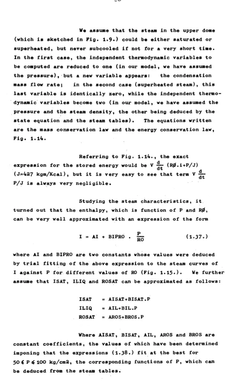
Ve assume that the steam in the upper dome (which is sketched in Fig. 1.9«) could be either saturated or superheated, but never subcooled if not for a very short time. In the first case, the independent thermodynamic variables to be computed are reduced to one (in our model, we have assumed the pressure), but a new variable appears: the condensation mass flow rate; in the second case (superheated steam), this last variable is identically zero, while the independent thermo­ dynamic variables become two (in our model, we have assumed the pressure and the steam density, the other being deduced by the state equation and the steam tables). The equations written are the mass conservation law and the energy conservation law, Fig. 1.14.

Referring to Fig. 1.14·, the exact expression for the stored energy would be V ­—■ (RØ.i+P/J)

dt

(«1=427 kgm/Kcal), but it is very easy to see that term V ­—■ P/J is always very negligible.

Studying the steam characteristics, it turned out that the enthalpy, which is function of Ρ and R0, can be very well approximated with an expression of the form

I = AI + BIPRO . ^ Q (I.37.)

where Al and BIPRO are two constants whose values were deduced by trial fitting of the above expression to the steam curves of I against Ρ for different values of RO (Fig. 1.13·)· We further assume that ISAT, ILIQ and ROSAT can be approximated as follows:

ISAT = AISAT+BISAT.P ILIQ = AIL+BIL.P ROSAT = AROS+BROS.P

Vhere AISAT, BISAT, AIL, AROS and BROS are constant coefficients, the values of which have been determined imponing that the expressions (I.38.) fit at the best for

In Figs. I.l4., I.l6., 1.17«, the real values of these functions are compared with the value computed with expressions (I.38.); as can be seen, this fitting is quite satisfactory.

By introducing the Eqs.(I.38.)and(l.37·)into the energy equation and combining it with the mass conservation

(Fig. 1.10.), the energy equation can be reduced to the following form which is more suitable to the computer:

V BIPRO 4? = - AI.(X.(VR+VREQ)-VREQ-VC)) _at + (AISAT+BISAT.P).(VR+VREQ)) - VREQ (AI+BIPR0.(P/R0)) - (AIL+BIL.P).VC

(I.39.)

eq·

dRO dt

Eq. (I.39.) together with the mass conservation

= X (VR+VREQ)-VREQ-VC (1.40.)

constitutes the set of equations which is to be integrated to compute RO and Ρ in the upper dome. The only unknown left is VC which is computed as follows:

Κ . (RO-ROSAT) RO > ROSAT

WC = \ (1.41.)

RO ^ ROSAT

l

The value of K must be chosen high enough to prevent RO to become greater than ROSAT for a long time, (how it happens can be understood replacing Eq. (l.4l.) into (l.40.)); this is equivalent to assume that, as soon as the steam in the upper dome reaches the saturation conditions, the condensation prevents it from going deeply into the subcooled region, which seems reasonable as one regards a practical system.

dome i· at the saturation condition; in fact, in this case, for what has been said, RO at ROSAT ad Eq. (1.37) still gives an acceptable approximation of the steam enthalpy, as it can be seen in Fig. I.l8., where:

AI + BIPRO ' ROSAT(P)

is compared with ISAT(P) .

In practice, it seems that, at the frequencies of the transients which have practical interest, the steam in the UDper dome is very near to the saturation condition being always a little superheated, and this is the reason why the system is not affected by the value of K.

d) Superheater

It has been supposed to make a negligible error assuming to have the same mass flow rate of steam along the whole superheater; this is true in steady state, while in transient, according to the mass conservation law, there are local variations due to the steam density variations in time:

— " - A ff · ax dt

It was nevertheless verified that, for cases of practical interest, the maximum flow variation in the cell

due to density variation remains below i% of the total flow·

The mass conservation law is thus reduced

to the trivial form V(i) - VREQ, where V(i) is the mass flow rate

th

in the i cell and VREQ the mass flow rate into the turbine.

1 Fig. 1.19«, the values of the steam density in the different cells and at different powers have been plotted; from this figure, one cou'd have the impression that the error committed in neglecting the density variations due to pressure and temperature variations is not too small.

In reality, looking at the equations, it is clear that the only effect of an error over RO is to modify the time constant between the temperature of the wall and the

temperature of the steam,and the effect on the primary side is still attenuated by the time constant between the organic temperature and the wall temperature.

Two transients done, assuming for RO values ten times greater and ten times smaller than the real ones, have shown no appreciable variations in the system behavior. This is due to the fact that, being always very near to the steady conditions, the error over RO is highly attenuated by the very little value of d "f1* (see Fig. 1.18.).

at

The energy conservation law has been written assuming, as thermodynamic independent variables, the pressure Ρ and the steam enthalpy H(i). For the pressure, we assume that it is the same as in the upper dome (we neglect the pressure losses due to friction and acceleration). The error we do in this way effects the calculation of the temperature of the steam in the cell and can be estimated at approximately 0.5°C, as can be deduced from Fig. 1.20., assuming that the pressure losses over each cell can be evaluated to 0.5 kg/cm2.

The steam temperature which appears on the right hand side of the energy conservation law (Fig. 1.18.) has been considered a dependent variable whose value is deduced from the steam enthalpy I and pressure Ρ with the following approximate formula:

T(°C) = i,3333 I + 1.0337 Ρ - 686.64 (1.42.)

In Fig. 1.20., the values of the steam

temperature against the steam enthalpy for different pressures

have been plotted together with the values corresponding to

Eq. ( 1 . 4 2 . ) .

As it can be seen, the approximation is

good, or at least comparable with the precision one can reach

in computing the heat transfer coefficients, provided one

remains in the region from 50 to 100 kg/cm 2 for the pressure,

and between 2 5 % and 110% of nominal power.

1.4. The control and regulation system

1.4.1. Requirements

The automatic control and regulation system

must stabilize the reactor which is instable with respect to

temperature coefficients, and adjust its power level to the

power demand according to a certain steady­state program.

1.4.2. Regulator equations and block diagram

Experiments on the analogue computer have

shown that the regulation mechanism must be driven by an error

term which should be a combination of two variables: the

neutron power and the average temperature of the organic coolant:

n­η PV ­ PV τ Τ ­Τ

av avo

r n­n FW ­ PW η

--■»[τ* - -ur-*]

-*.

·» ο ο J

Τ (1.43.)

ο Ί avo

where:

£, is the actuating error n is the neutronic power

PV is the power demand at the turbine

Τ » (temperature primary at the inlet of the heat a v exchanger + temperature primary at the outlet

of the heat exchanger)/2

Note that Τ represents the average temperature only under steady­state conditions

R and R are arbitrary gains to be optimized

1 2

η , PV , Τ are the values of N, PV, Τ at the nominal

o o' avo av

power of the reactor; they can be functions of the power

n­η PV­PV

The terms ° and ■_, ­ allow to compare

n FW

o o

the extracted power of the reactor to the power supplied to the turbine and to adjust one to the other. The power demand PV is the product (VREQ.AH) where VREQ is the steam flow and AH the enthalpy span from the superheating steam temperature to the

economizer water input temperature (which is assumed to be œnstant according to the reactor power)· The power demand PV is changed by acting the steam throttle at the turbine input, which is

identical to modifying the steam flow, but in a manner to verify the previous equality.

The term in n compensates the fast variations of the power, which are impossible to correct with temperature

signals due to the important time delays (time delay in transferring the heat from fuel to coobit: about 3 sec. and transport delay

time to the mixing main collector: about 10 sec·)·

The term in T corrects any variation of av

the average temperature; by definition, this is a low­frequency action and has little effect on the stability of the system, but influences greatly the variation of the thermodynamical quantities of the heat exchanger.

To the error term must be added a pressure p"Po

term defined as ­ R — — an<i intended to improve the pressure

J Po

regulation program). Τ and ρ are two thermodynamical avo o

parameters connected so that the pressure term acts in the opposite direction of the term in T ; therefore, its weight

av

must be limited· This situation derives from the fact that a regulation program for a multiple-loop system is necessarily a compromise between contradictory requirements.

The control-rod mechanism is represented by the following transfer function:

where:

Ρ is the reactivity introduced by the control mechanism

S is the differential operator -rr (Laplace operator)

at

* is the time constant due to the intertia of the

mechanism

R, and R are arbitrary gains to be optimized

Thus, the position of the control rod is changed in proportion to any error created by a power demand change or by an internal system transient. An on-off type

control rod is inadequate, the reactor by itself being inherently instable; the presence of a dead zone in that discontinuous type system causes the control system to be in continuous oscillation.

The regulation is linear only within limits imposed by technology, which must be taken into account:

- the speed of the control rod has a sharp maximum limitation:

d * •

-~ -^ max. speed of rods _at

- the end-of-run limitations of the control rods must be considered as well:

Ρ ^. max. available reactivity

The law of variation of reactivity versus rod displacement is assumed to be linear for the computation, as it was verified on the computer that (within the limits sentioned

above) any alternative (section of a sine function) does not change significantly the behavior of the control loop.

A separate mean to set the equilibrium point at any desired value between these limits must be avail -able·

It must be remembered that, if a reactivity disturbance greater than the above value occurs for any

significant length of time, the regulator looses its ability to control the reactor·

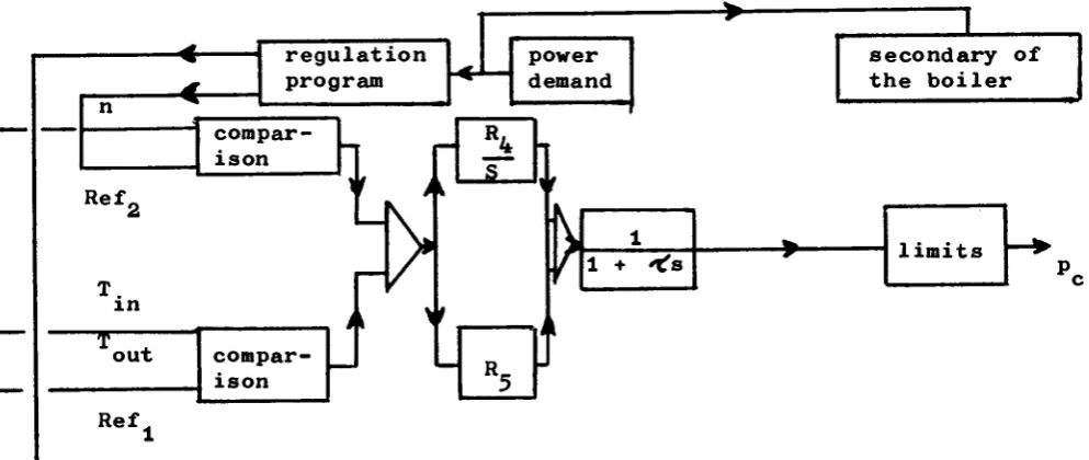
The block diagram for the whole power plant control is reported on Fig. 1.21. The detail of the regulator is given in Fig· b. and Fig. c , which represent two possible servo mechanisms being mathematically equivalent. In Fig. b., the actuating error is integrated through an electronic

integrator; its output and the error signal itself drive the control mechanism which acts here as a position servo. In Fig. c , the error signal and its derivative (damping term) drive a bar mechanism which is a rate servo.

Eliminating 6. between the relatione (1.43·) and (1.44.), it appears that the proportional and integral terms are affected to the variables η, Τ and, eventually, p.

av * '

Generally, the proportional terms are the stabilizing terms (the terms which improve the transients); the integral terms are the reset terms (refer to analogue and analytic results).

a) Minimum overshoot of all variables in transient response, in particular with respect to reactivity disturbances«

b) Minimum time for passing from one steady state to another when the power demand is varied·

c) Minimum time to return to steady state after any disturbance«

I.4.3. The steady-state program

In Fig. 1.21., a regulation program sets the sum of the reference terms of the Eq. (1.43* ): n and PV

^ 0 0

are constants, while Τ and ρ may vary according to a certain avo o

predetermined law (steady-state program) as a function of PV; it will be recalled that Τ and ρ naturally will always remain

avo o

thermodynamically connected. One of the possible steady-state programs of the power plant is reported in Fig. 1.22. (program l); - From 100% to 75% of the power, the average temperature of the

coolant remains constant; the steam pressure rises from 5315 kg/cm2 to 67 kg/cm2. This range of power is considered to be the normal working zone of the plant.

- From 75% to 25% of the power, the steam pressure is maintained constant; the average organic temperature decreases from 308°C to 289°C.

The inlet and outlet temperatures of the coolant are represented on Fig. 1.22. in the same way as the steam inlet temperature at the turbine. Let us remember that the assumed steam cycle taken into account for the dynamics calculations is without reheating.

Experimentation made on computer has shown that many alternatives, all stables, are possible; in each case, the regulation can be driven by Τ (R„ = 0 ) , assuming a

av 3

variable reference Τ which depends on the power demand as in avo

Fig. 1.22.; an additional term in ρ - ρ (R =0) where ρ depends on the power demand as in Fig. 1.22. always improves the

The regulator reference is setting to the predetermined law (as a function of the power demand signal) by a program (see Fig. 1.21a) which could be a set of relays, comparators and constant gain amplifiers wired in a permanent arrangement or, for more flexibility, a small on-line computer

(digital or analogue).

Other static programs studied are reported in Fig. I.23. The numerical differences between the two

programs 1 are explained by the fact that the dynamical studies have been executed on two prototype variants where the coolant organic span is, either 124°C (Fig. 1.22.), or 104°C (Fig. 1.23.); in this last case, the steam pressure rises from 60 to 74 kg/cm2 when the power decreases from 100% to 75%· The results of the

study are modified in no way.

2. The analogue computation results

2.1. The instable core

2.1.1. Main characteristics of the channel

Bundle 19 rods Fuel cross-section 31 cm2 Coolant cross-section 22 cm2

Moderator area/coolant area ratio 1516 Length channel 400 cm

Fuel rod radius 1*45 cm Cladding wall thickness 0,88 mm

Finning ratio 1,9 Thermal resistance between fuel & cladding l,5°C/w/cm2

Maximum integral of conductibility 100 w/cm Average velocity in the central channel 10 m/sec

Characteristics of the "representative" channel (the power

of which being 0,89 the power of the central channel) at

nominal power

Removed power 4,65 MW

Input temperature 266°C

Output temperature 370°C

Average cladding temperature T_ 376°C

G

Average fuel temperature Τ 672,5°C

Temperature coefficients of the initial core:

- Fuel temperature coefficient: °t = - 1,5 pcm/°C

- Coolant temperature coefficient: oi. = - 0,25 pcm/°C c

Temperature coefficients of the equilibrium core:

- Fuel temperature coefficient: o< = - 0,45 pcm/°C

- Coolant temperature coefficient: c< = + 5,6 pcm/°C c

Transport delays of coolant from

reactor to heat exchanger: 12 and 13 sec.

2.1.2. The reactor stability

The prototype stability situations have been

studied in the parametric plane ( + <?¿ , - o¿ ) , examining

coolant fuel

the open loop transient response of the reactor to an initial

positive step disturbance of 50 pern. If the second derivative

of neutron power versus time is negative, after a time of 100 sec.

longer than the longest time constant, the reactor is considered

to be stable.

The results are reported in Fig. 1.24. for

the two cases of a thermal resistance of 1.5°C/w/cm2 and

0.5°C/w/cm2 (the two curves are identical).

One can see that the irradiated reactor is

unstable. Thus the prototype requires an automatic external

2.1.3» Optimization of the regulator parameters

After experimentation, the following numerical values have been retained (if no speed limitation on control rod):

R, = 10 m 10 pcm/% variation

R » 5*10~ ■ 50 pcm/% variation

5

ν , . ι ^ 2 sec *v inertia

The regulator inertia K. .. = 2 sec. was inertia

used for computation as a worst case value.

Fig. 1.25« gives the stability domain of the control mechanism versus the gains R, and R , in the linear region of its transfer function (i.e. for disturbances which do not reach the reactivity speed and amplitude limitation). In the region to the left, the mechanism is stable and gives a damped response to a step input. In the central region, the mechanism is stable but gives a periodical response (overshot) to a step disturbance. In the right region, the loop is unstable·

The working point of the controller should be selected in the first region (damped). In fact, in order to avoid overshots in the non­linear region, systematic experimental investigation has shown that the working point of the mechanism should be about a decade to the left of the critical damping line as, for example, point l6 if the insertion speed of reactivity is limited to 10 pcm/sec.

Fig. I.26. and 1.27* give the response of the system in case of a step disturbance of 50 pern considered as a worst case for a small accident (like the drop of a cluster in the channel during the fuel handling), not requiring a scram.

Fig. 1.26. for a speed limitation of the control rods of 10 pcm/sec (equivalent to 10 cm/sec) and a rod inertia time constant of 2 sec.

Fig. 1.27* for an unlimited speed of the control rods·

During these transients, the temperatures do not change significantly.

2.1.4. Ability of the regulator to control the reactor

The regulator optimized for values of

temperature coefficients corresponding to the irradiated reactor, it is interesting to investigate up to which extreme limits the regulator is capable to keep the reactor under control. The quantities which affect significantly these limits are:

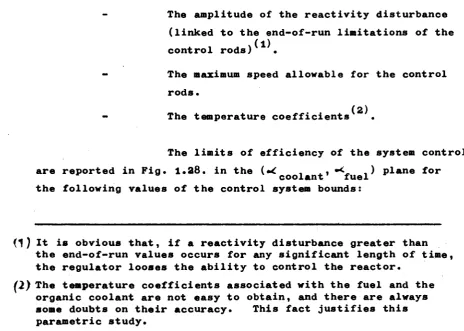
The amplitude of the reactivity disturbance (linked to the end-of-run limitations of the control rods) .

- The maximum speed allowable for the control rods.

(2) The temperature coefficients

The limits of efficiency of the system control are reported in Fig. 1.28. in the (*¿ , . , ·<_ .) plane for

w coolant' fuel

the following values of the control system bounds:

(1) It is obvious that, if a reactivity disturbance greater than the end-of-run values occurs for any significant length of time, the regulator looses the ability to control the reactor.

(2) The temperature coefficients associated with the fuel and the

Maximum rods speed: 15 cm/sec (e.g. 15 pcm/sec) Rod reactivity span from + 200 pern to - 300 pem with two sets of four rods: the negative reactivity end-of-run of the normal first set

(-50 pem) commands the release of the second group of rods (-250 pem) (see Fig. 1.29·). The time constant of rods was taken = 1 sec.

for this investigation.

Curves 1 and 2 give the limit above which a reactivity step disturbance of 100 and 50 pem cannot be compensated by the regulator; curves 3 and 4 give the same limit for a step disturbance in the reactor inlet temperature of 10°C and 5°C respectively.

It turned out that the speed would be

sufficient to control the system up to very high values of°* ,

c

if the amount of reactivity supplied by the regulator is adequate· Beyond the limits of curves 1 to 4, the regulator looses its

ability to control the reactor for the described disturbance·

2.1.5. Heat exchangers: accuracy of the dynamic computations - Steady-state checks

The steady-state results have been obtained for 100% and 75% of full power, as the equilibrium values of the dynamic equations. The steady-state temperature distribution for the heat exchanger is reported in Fig. I.30. for 100% power, and Fig. I.31. for 75% power. These results have been compared with those of a purely static digital computation (using thus a different mathematical representation. The agreement (within some degrees centigrades) between the results of the two