CAS: Embedded Predictive Analysis of Misrepresentation Risk in GLM Ratemaking Models

of Misrepresentation Risk

in GLM Ratemaking Models

by Michelle Xia, Lei Hua, and Gary Vadnais

ABSTRACT

Misrepresentation is a type of insurance fraud that happens frequently

in policy applications. Due to the unavailability of data, such frauds

are usually expensive or difficult to detect. Based on the distributional

structure of regular ratemaking data, we propose a generalized linear

model (GLM) framework that allows for an embedded predictive

analysis on the mis representation risk. In particular, we treat binary

misrepresentation indicators as latent variables under GLM ratemaking

models for rating factors that are subject to misrepresentation. Based on

a latent logistic regression model on the prevalence of misrepresentation,

the model identifies characteristics of policies that are subject to a high

risk of misrepresentation. The method allows for multiple factors that

are subject to misrepresentation, while accounting for other correctly

measured risk factors. Based on the observed variables on the claim

outcome and rating factors, we derive a mixture regression model

structure that possesses identifiability. The identifiability ensures valid

inference on the parameters of interest, including the rating relativities

and the prevalence of misrepresentation. The usefulness of the method

is demonstrated by simulation studies, as well as a case study using the

Medical Expenditure Panel Survey data.

KEYWORDS

the partially identified parameters, even with an infinite amount of data.

Proposed by Brockman and Wright (1992), GLM ratemaking models are now very popular in prop­ erty and casualty insurance areas (see Haberman and Renshaw 1996). In GLM ratemaking models, possi­ ble misrepresentation in a rating factor is expected to cause an attenuation bias in the estimated risk effect (e.g., the relativity), resulting in an underestimation of the difference between the true positive and true negative groups. Despite discussions on operational changes in order to discourage such fraudulent behaviors, there seems to be little work concerning statistical models for predicting or evaluating the risks or expenses associated with such fraud. In Xia and Gustafson (2016), the authors studied the structure of GLM ratemaking models with a binary covariate (e.g., risk factor) that is subject to mis­ representation. The study revealed that all parameters are theoretically identifiable for GLM ratemaking models with common distributions assumed for claim severity and frequency. This suggests that we can esti­ mate the rating relativities consistently, using regular ratemaking data. However, the study was based on a simplified situation where there is a single risk factor subject to misrepresentation, without including other risk factors.

In the current paper, we use regular ratemaking data to develop GLM ratemaking models that embed predictive analyses of the misrepresentation risk. The particular extensions include: (1) the adjust­ ment for other correctly measured risk factors in the ratemaking model; (2) the incorporation of multiple rating factors that are subject to misrepresentation; (3) the embedding of a latent logistic model for how risk factors affect the prevalence of misrepresentation, which enables us to perform a predictive analysis (see Frees et al. 2014 and Shi and Valdez 2011) on the misrepresentation risk. We derive mixture regression structures for the conditional distribution of the observed variables, confirming the identifi­ ability of the models. We perform simulation studies based on finite samples, show that we can consistently

1. Introduction

For property and casualty insurance, ratemaking models are often determined using historical claim data based on rating factors that are predictive for loss severity and frequency. We refer to Klein et al. (2014), Bermúdez and Karlis (2015), David (2015), Hua (2015), Shi (2016) for illustrations in this regard. For example, auto insurance rates are usually calculated using risk factors such as use of vehicle, annual mile­ age, claim and conviction history, age, gender and credit history of the insured or the applicant (Lemaire et al. 2016). Due to the financial incentives, policy applicants may have a motivation to provide false statements on the risk factors. This type of fraud occurring on the policy application is referred to as insurance misrepresentation (Winsor 1995). In auto insurance, information regarding risk factors such as use of vehicle and annual mileage is generally hard to obtain. Even for insurers that offer a voluntary discount on mileage tracking, the existence of anti­ selection limits the capability of such programs in obtaining accurate information on the whole book of policies.

Denote q = P(V = 1), the true probability of a positive risk status. We can derive the observed prob­ ability of a positive risk status as q* = P(V * = 1) = P(V* = 1_V= 0)P(V = 0) + P(V* = 1_V= 1) P(V = 1) = q(1 − p). In insurance applications, a quantity of inter­ est is q = P(V = 1_V*= 0), the percentage of reported negatives that corresponds to a misrepresented true positive risk status. We define q as the prevalence of misrepresentation. Using the Bayes’s theorem, the prevalence of misrepresentation can be obtained as

1 * 0 * 0 1 1

* 0

1 1 .

P V V P V V P V

P V

p

p q

(

)

(

)

(

)

(

)

( )

= = = = = =

=

= θ

− θ − =

Similarly, we can obtain p = (1 − q)q/[q(1 − q)]. Note, we can derive one conditional probability from the other, along with an estimate of the observed probability q* using samples of V*. Note that the prevalence of misrepresentation q represents the per­ centage of misrepresented cases among applicants who reported a negative risk status. It quantifies the misrepresentation risk of a particular application and thus determines the total number of misrepresented cases in the book of business.

In a GLM ratemaking model, the model considers the mean of a response variable Y from a loss or count distribution, conditioning on the true risk status V. In Xia and Gustafson (2016), the authors showed that the conditional distribution of the observed vari­ ables (Y_V*= 0) is a mixture of the two distributions of (Y_V= 0) and (Y_V = 1), and (Y_V*= 1) has the same distribution as (Y_V = 1). Since one of the two mixture components can be informed from data with V* = 1, the mixture model possesses the model identifiability in a general case when the response variable is non­binary. Furthermore, the authors showed the moment identifiability of the model by deriving the observable moments corresponding to Y and V*. In an identified model, the likelihood func­ tion possesses one unique global maximum, allowing estimate the model parameters including the rating

relativities, and interpret how risk factors affect the prevalence of misrepresentation. The case study using the 2013 Medical Expenditure Panel Survey (MEPS) data illustrates the use of the proposed method in an insurance application.

The proposed model is expected to have an imme­ diate impact on the actuarial practices of the insurance industry. Based on the theoretical identification of the model, traditional GLM ratemaking models can be extended to embed a predictive analysis of mis­ representation risk without requiring extra data on the misrepresentation itself. The analysis will pro­ vide information on the characteristics of the insured individuals or applicants who are more likely to mis­ represent on self­reported rating factors. With pre­ dictive models that automatically update with new underwriting data, the prevalence of misrepresenta­ tion can be predicted at the policy level, during policy underwriting based on various risk characteristics. Therefore, underwriting interventions can be under­ taken in order to minimize the occurrence of mis­ representation. In addition, the claims department may use the risk profiles to help identify fraudulent claims.

2. A GLM ratemaking model

with misrepresentation

In Xia and Gustafson (2016), the authors studied the identification of a GLM when a covariate (e.g., a rating factor) is subject to misrepresentation. For misrepresentation in a binary rating factor (e.g., smoking status), we can formulate the model as follows. Denote by V and V * the true and observed binary risk status, respectively. There is a chance for misrepresentation to occur if the individual has a positive risk status. In particular, we can write the conditional probabilities as

* 0 0 1

P V

(

= V=

)

=

* 0 1 , (1)

P V

(

= V= =

)

p

Given fixed values of x, the conditional distribution of (Y_V *, x) is a mixture of two distributions when V *= 0, and it is a single distribution when V * = 1. The mixture model in (2) with additional covariates x is called a mixture regression model. Such mixture models have been shown to possess identifiability, given that a mixture distribution is identifiable for the specific component distribution (see Hennig 2000, and Grün and Leisch 2008b). Owing to the identifi­ ability for mixtures of distributions from the expo­ nential family (Atienza et al. 2006, 2007), the model in Equation (2) will be fully identifiable for common loss severity and frequency distributions such as the gamma, Poisson and negative binomial distribu­ tions considered under the GLM ratemaking context. Hence, using regular ratemaking data containing (Y, V *, x), we can consistently estimate the mixture weight q (i.e., the prevalence of misrepresentation), and the regression coefficients in ` (and the cor­ responding relativities).

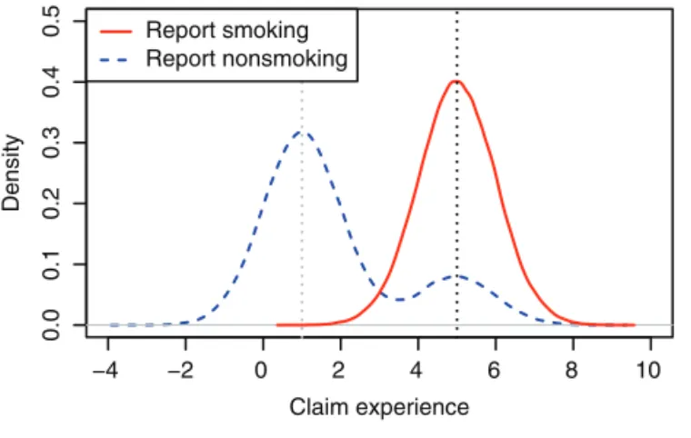
In order to understand the model identification, we use a hypothetical example to visualize the con­ ditional distribution of (Y_V *, x) under the mixture regression context. For better visualization of the mixture structure, we assume that the medical loss amount Y follows a lognormal distribution, with V * being the smoking status. Given x=x0 (i.e., assum­

ing that the comparison is among individuals with the same other risk factors), (log(Y )x=x₀) will have a mixture of two normal distributions for individuals who reported non­smoking, while it will have a normal distribution for those who reported smoking. Figure 1 gives an example on how the conditional distributions look like, with x = x₀ being fixed for both groups. For the dashed density, the two mixture components are the conditional distributions for the true nonsmokers and smokers, and the preva­ lence of misrepresentation is the mixture weight for the true smokers that has a higher mean. Note that in the mixture regression model, the two components are regression models that cannot be visually presented, although the model possesses the identifiability for estimating all parameters. This mixture regression consistent estimation of all parameters including p

and q. This means we can consistently estimate the true relativity and the probability p with regular rate­ making data. Here, we will extend the work under the GLM ratemaking framework in three directions: (a) to include additional rating factors that are correctly measured, a situation we commonly face in insurance ratemaking; (b) to simultaneously include multiple rating factors that are subject to misrepresentation; and (c) to relax the assumption that the prevalence of misrepresentation does not change with values of rating factors.

2.1. Model with correctly

measured risk factors

In the GLM ratemaking model, we first assume that the loss outcome Y depends on the true status V. In order to formulate the problem for the first exten­ sion, we use x= (X₁, X₂, . . . , X_K) to denote K correctly measured rating factors that are predictive of the loss outcome Y. The GLM ratemaking model can be written as

. . . _,

0 1 1 1

g

( )

µ = α + αX + + αKXK+ αK+V

where µ= E(Y) and Var(Y ) =jV(µ), with j being the dispersion parameter and V(•) being the variance

function. Denote ` = (α0, α1, . . . , αK+1), and let i

denote all other parameters including the dispersion parameter. We may use f_Y(y_`, i, V, x) to denote the conditional distribution function of (YV, x) from the exponential family.

Assume that the misrepresentation is non­differential on Y (i.e., Y ⊥ V *_V, x). That is, the outcome Y does not depend on whether the applicant misrepresents on the risk factor, given the true status V and other risk factors x. We can obtain the conditional distribution of the observed variables, (Y_V *, x), as

* 1, , , 1,

* 0, , , 1,

1 , , 0, . (2)

x x

x x

x

f y V f y V

f y V q f y V

q f y V

Y Y

Y Y

Y

(

)

(

)

(

)

(

)

(

) (

)

= = =

= = =

i=j. Note that p and q are parameters of the model, for which we can perform inference using either frequentist or Bayesian approaches. For Bayesian methods, the posterior distributions of ( p_V *,x) and (qV *,x) do not have closed forms. Hence, we will need to use Markov chain Monte Carlo (MCMC) tech­ niques in order to make inference on the parameters.

2.2. Multiple risk factors

with misrepresentation

For the second extension, we denote v = (V₁,

V₂, . . . , V_J) as the true status of J rating factors

that are subject to misrepresentation, and v* = (V₁*,

V₂*, . . . , V*) as the corresponding observed values _J

for these rating factors. We may assume that the response variable Y depends on the rating factors v

through a parameter vector ` (e.g., one intercept and J regression coefficients). We further assume that (Y<sub></sub>v) has the probability function f<sub>Y</sub>( y<sub></sub>`, i, v). Under the assumption of non­differential misclassi­ fication, the conditional distribution of (Y_v*) will either be a single distribution when v* = (1, 1, . . . , 1), or a mixture distribution with the number of com­ ponents and the mean of components determined by the values of the observed v*. For example, when there are two rating factors with misrepresentation (i.e., v= (V₁, V₂)), we can write the conditional dis­ tribution of observed variables, (Y_v*), as

* 1, * 1 , , 1, 1

* 0, * 1 , , 1, 1

1 , , 0, 1

* 1, * 0 , , 1, 1

1 , , 1, 0

* 0, * 0 , , 1, 1

, , 0, 1

, , 1, 0

1 , , 0, 0 (4)

1 2 1 2

1 2 1 1 2

1 1 2

1 2 2 1 2

2 1 2

1 2 3 1 2

4 1 2

5 1 2

3 4 5 1 2

f y V V f y V V

f y V V q f y V V

q f y V V

f y V V q f y V V

q f y V V

f y V V q f y V V

q f y V V

q f y V V

q q q f y V V

Y Y Y Y Y Y Y Y Y Y Y Y Y

(

)

(

)

(

)

(

)

(

) (

)

(

)

(

)

(

) (

)

(

)

(

)

(

)

(

)

(

) (

)

= = = = = = = = = = + − = = = = = = = + − = = = = = = = + = = + = = + − − − = =

structure allows us to estimate the mixture weight (the prevalence of misrepresentation), the true risk effect of smoking (i.e., the difference in the mean of the two components), and the regression coefficients associated with each of the risk factors in x, without observing V.

Example 2.1. (Gamma model) First, we give a simplified example of a gamma loss severity model commonly used for auto insurance. Denote by Y the amount of a liability loss for a given claim, by X the annual mileage traveled by the vehicle, and by V* the observed risk status on vehicle use status (e.g., business or not) that is subject to misrepresentation. We can use a gamma GLM severity model given by

, gamma ,

log

* , Bernoulli 1 , (3)

,

, 0 1 2

∼

∼

Y V X

V X

V V X p V

V X V X

(

)

(

)

(

)

(

)

(

)

(

)

ϕ µ

µ = α + α + α

−

where j is the shape parameter, and µ_V,X is the conditional mean of the gamma distribution given V and X. Note that the conditional distribution of the observed variables (YV*, x) have the same form as that in Equation (2). For this example, the conditional distribution f_Y(y`, i, V, x) takes the form of the above gamma distribution, with `= (α0,α1,α2) and

−4 −2 0 2 4 6 8 10

0.0 0.1 0.2 0.3 0.4 0.5 Claim experience Density Report smoking Report nonsmoking

identifiability of mixture regression models (Hennig 2000, and Grün and Leisch 2008b), the model in (4) is identifiable for the common loss severity and fre­ quency distributions assumed in a GLM ratemaking model. This means all the regression coefficients in ` (and the corresponding relativities), and the mixture weights (i.e., prevalence of misrepresentation q_j, j= 1, 2, . . . , 5) can be consistently estimated from regular ratemaking data containing (Y, v*). The results can be extended straightforwardly to the case with more than two rating factors subject to misrepresen­ tation. Note that the distributional assumptions we adopted in the two previous paragraphs are for the purpose of obtaining analytical forms of the preva­ lence of misrepresentation q_j’s. The identifiability of the model is obtained from the mixture structure we have in (4) and does not depend on the specific forms of q_j’s.

Example 2.2 (Negative binomial model) We give an example of a negative binomial loss frequency model commonly used for auto insurance. Denote by Y the number of liability losses for a given policy year, and by (V₁*, V₂*) the observed risk status on the binary vehicle use and binary annual mileage (e.g., on whether it is over a certain threshold) that are subject to misrepresentation. In particular, we can write the negative binomial GLM model as

1, 2 negbin ,

log , (5)

,

, 0 1 1 2 2 1 2 1 2

∼

Y V V

V V

V V

V V

(

)

(

)

(

)

ϕ µ

µ = α + α + α

where j is a dispersion parameter and µ_V1,V2 is the conditional mean of the negative binomial dis­ tribution given the true statuses (V₁, V₂). Note that the conditional distribution of the observed variables (YV₁*, V₂*) have the mixture structure given in Equa­ tion (4), and the prevalence of misrepresentation q_j’s are the mixture weights that can be estimated using data on (YV₁*, V₂*). For this example, the condi­ tional distribution f_Y ( y_`, i, V₁, V₂) takes the form of the above negative binomial distribution, with

`= (α0, α1, α2) and i=j.

where the corresponding prevalence of misrepresen­ tation q₁= P(V₁= 1, V₂= 1_V₁* = 0, V₂* = 1), q₂= P(V₁= 1, V₂= 1V₁* = 1, V₂* = 0), q₃ = P (V₁ = 1, V₂= 1_V₁* = 0, V₂* = 0), q₄= P(V₁= 0, V₂= 1_V₁* = 0, V₂* = 0) and q₅= P (V₁= 1, V₂= 0V₁* = 0, V₂* = 0).

In order to simplify the model, we may assume that there is no correlation in the two risk factors, and the occurrence of misrepresentation in one risk factor does not depend on the value or the mis­ representation status of the other. That is, we have V₁⊥ V₂, P(V₁* = 0_V₁= 1, V₂) = P(V₁* = 0_V₁= 1) = p₁, P(V₂* = 0V₁, V₂ = 1) = P(V₂* = 0V₂= 1) = p₂, and P(V₁* = 0, V₂* = 0V₁ = 1, V₂ = 1) = p₁p₂. Denote P(V₁= 1) =q1 and P(V2= 1) =q2. Using Bayes’ theo­

rem, we derive specific forms of the prevalence of misrepresentation, the q_j’s, in the Appendix. In par­ ticular, q₁ and q₂ have the same form as q in Equation (2). That is, q_j=qjpj/[1 −qj(1 − pj)], j = 1, 2. In addi­ tion, we have q₃= p₁p2q1q2/[p1p2q1q2+ p1q1(1 −q2) +

p₂(1 – q1)q2 + (1 – q1)(1 – q2)], q4 = p2(1 − q1)q2/

[p₁p₂q1q2 + p1q1(1 − q2) + p2(1 − q1)q2 + (1 − q1)

(1 – q2)], and q5= p1q1(1 – q2)/[p1p2q1q2+ p1q1(1 −q2) +

p₂(1 −q1)q2+ (1 −q1)(1 – q2)].

An alternative to the above conditional indepen­ dence assumption is the assumption on the preva­ lence of misrepresentation, the q_j’s. For example, we can assume that the applicant has the same mis­ representation probability p₁ = p₂ for the two risk factors. When the true status is positive for both risk factors, it is reasonable to assume that there are only two possibilities on the misrepresentation status: the applicant either does not misrepresent on any risk factor, or misrepresents on both of them. That is, we have the prevalence of misrepresentation being q₄= q₅= 0. In such a case, the last mixture distribu­ tion in (4) will only have two components. This will dramatically simplify the model when there are more than two risk factors subject to misrepresentation.

where µ_V,X is the conditional mean of the Poisson distribution given the true status (V, X). Note that the conditional distribution of the observed variables (YV *, x) have the same form as that in Equation (2), except for the fact that q varies with the covariate X. Here, the logit model on q is a latent model that requires no additional information other than observed data on X. For this example, the conditional distri­ bution f_Y( y_`, i, V, x) takes the form of the above Poisson distribution with `= (α0, α1, α2), and there is

no parameter i needed for the Poisson model.

When there is a latent binomial or multinomial regression model (6) on the mixture weight q, the mix­ ture in (2) is called a mixture regression model with concomitant variables (see Grün and Leisch 2008a). According to Hennig (2000) and Grün and Leisch (2008b), such a mixture regression model is identifi­ able, provided that a simple mixture of the component distributions is identifiable. The identifiability will ensure that we would be able to make inference on how different characteristics (e.g., demographics and other risk factors) affect the prevalence of mis­ representation q. Based on the conditional distribution of the observed loss outcomes and risk factors, the model will require no extra data on the misrepresen­ tation itself.

Owing to the identifiability, we will be able to estimate the regression coefficients a for the latent model on the prevalence of misrepresentation using regular ratemaking data. The statistical significance of the variables indicates what characteristics of the applicants or insureds affect the probability that a reported negative risk status corresponds to a mis­ represented true positive status. Using such estimated predictive models that automatically update with new loss experience data, the prevalence of misrepresenta­ tion can be predicted at the policy level, during policy underwriting based on various risk characteristics. The applications with a high predicted prevalence of misrepresentation can then be selected for an under­ writing investigation on self­reported risk factors. For the claims department, the predicted prevalence of misrepresentation can be used as a flag for identi­ fying potential fraudulent claims. Such a risk profile

2.3. Embedded predictive analysis

on misrepresentation risk

The last extension is very important for understand­ ing the characteristics of the insureds or applicants who are more likely to misrepresent on certain self­ reported rating factors. In addition to the regression relationship we are assuming between the mean of the loss outcome and the rating factors, we may further assume that the prevalence of misrepresentation q depends on certain risk factors. Without loss of gen­ erality, we assume the case in Equation (2) where there is one variable V subject to misrepresentation. Like in the case of zero­inflated regression models (see, e.g., Yip and Yau 2005), we may use a latent binary regression model for the relationship between the prevalence of misrepresentation and the rating factors. That is,

, (6)

0 a

g q

( )

= β +z

where the link function g(•) can either take the logit

or probit form, β0 is an intercept and the vector a con­

tains the effects of the rating factors on the prevalence of misrepresentation. For the latent model in (6), it usually requires a larger sample size to learn param­ eters with the same precision. In order to simplify the model in real practices, we recommend choosing a subset of meaningful risk factors from x such as z, in the case where there are many rating factors available.

Example 2.3 (Poisson model). We give an example of a Poisson loss frequency model commonly used for auto insurance. Denote by Y the number of liability losses for a given policy year, by V * the observed risk status on the binary vehicle use status with possible misrepresentation, and by X the annual mileage. In particular, we can write the Poisson GLM model as

, Poisson

log

logit log

1 , (7)

,

, 0 1 2

0 1

Y V X

V X

q q

q X

V X

V X

(

)

(

)

(

)

( )

µ

µ = α + α + α

=

− 

  = β + β

, , , * log

1 * 1 log 1

log ,

0 1 2 1 2

1

2 1

l v y

v z q y

z q y

i i

i n

i

i i

i i

i n

∑

∑

[

]

[

]

(

)

( )

(

)

(

) ( )

( )

( )

α α α ϕ = φ

+ − − − φ

+ φ

   

   

=

=

where φ1( yi) = f ( yivi= 0, xi) is the conditional dis­ tribution for the regression model of the true non­ smokers, and φ2( yi) = f ( yivi = 1, xi) is that of the true smokers.

Note that regular GLM can be implemented either using the frequentist approach based on maximum likelihood estimation (MLE) or Bayesian inference based on MCMC. This is true for the proposed model as well. For the current paper, we use Bayesian infer­ ence that is convenient to conduct, as well allowing prior information to be incorporated on the param­ eters of the interest, when external information is available. Information regarding likelihood­based inference based on the EM algorithm as well as that regarding the complete­data likelihood function can be found in standard references such as McLachlan and Krishnan (2007).

Treating z_i (i = 1, 2, . . . , n) as latent variables, the Bayesian models can be implemented in the soft­ ware package R using MCMC methods such as the Metropolis­Hastings algorithm (as was done in Xia and Gustafson (2016). In addition, we may use Bayesian software packages such as WinBUGS and OpenBUGS to implement the models, by introduc­ ing a latent status on misrepresentation. In particular, the BUGS code for implementing the gamma model in Example 2.1 is as follows.

model {

for (i in 1:n){

V_star[i] ~ dbin(theta_star,1) Y[i] ~ dgamma(alpha, beta[i])

beta[i] <- alpha/exp(aa0 + aa1*V[i] +

aa2*X[i])

V[i] <- V_star[i] + (1-V_star[i])*Z[i] Z[i] ~ dbin(q,1)

}

theta_star <- theta*(1-p) q <- theta*p/(1-theta*(1-p))

based on the predicted prevalence will be helpful for identifying misrepresentation on policy applications, as well as fraud in insurance claims.

3. Simulation studies

We perform simulation studies on the performance of the model under finite sample scenarios, in order to illustrate the model identifiability. In particular, we study the model performance under three scenarios where we have (1) another correctly measured rating factor, (2) multiple rating factors subject to misrepresentation, and (3) a misrepresented rating factor with the prevalence of misrepresentation vary­ ing with other factors.

3.1. Model implementation

The proposed models given in Equations (2) to (7) all have tractable analytical forms. Hence, we can write out the full likelihood functions. For the model implementation, it is more convenient to work with the complete­data likelihood with a latent variable denoting the misrepresentation status.

Here, we use the gamma loss severity model in Example 2.1 to illustrate the implementation of the proposed models. Denote by ( y₁, v₁*, x₁), (y₂, v₂*, x2), . . . , ( yn, vn*, xn) a random sample of observed variables of size n. Maximum likelihood estimation (e.g., based on the expectation maximiza­ tion algorithm, EM, McLachlan and Krishnan 2007) and Bayesian inference (based on MCMC) uses the complete­data likelihood that includes the unobserved (i.e., latent) status on the misrepresentation. For observations where v* _i = 0, denote by z_i(i = 1, 2, . . . , n) the latent binary indicator on whether Observation i is misrepresented (whether the true status v_i= 1, i.e., whether Sample i is from the component distribu­ tion for true smokers).

for obtaining the corresponding samples of V *. The samples of the additional factor X are generated from a gamma distribution with the shape and scale param­ eters being (2, 0.5). The corresponding samples of Y are then generated from those of V and X, with regres­ sion coefficients (α0, α1, α2) being (1.2, 1, 0.5), and a

gamma shape parameter j= 5.

For the simulation study, we consider the five sample sizes of 100, 400, 1,600, 5,400, and 25,600. We compare the results from the proposed model in (2) with naive estimates from gamma regression using the observed values of V *, pretending there to be no misrepresentation. We denote the true model as gamma regression using the “unobserved” values of V that we used earlier for obtaining the samples of V *. For all the models, independent normal priors with mean 0 and variance 10 are used for the regression coefficients. For the probability parameters q and p, uniform priors on (0, 1) are used. We run three chains with randomly generated ini­ tial values. The first 15,000 samples are dropped to ensure that the Markov chain has converged. In order to reduce the autocorrelation in the posterior samples, we take every 10th sample for our model acknowledging misrepresentation. For all the other models with faster convergence, we take every 10th sample after dropping the first 1,500 samples.

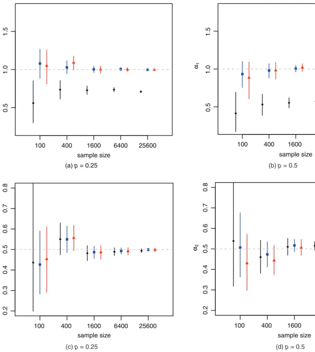
Figure 2 presents the 95% equal­tailed credible intervals for the regression effects α1 and α2 of the

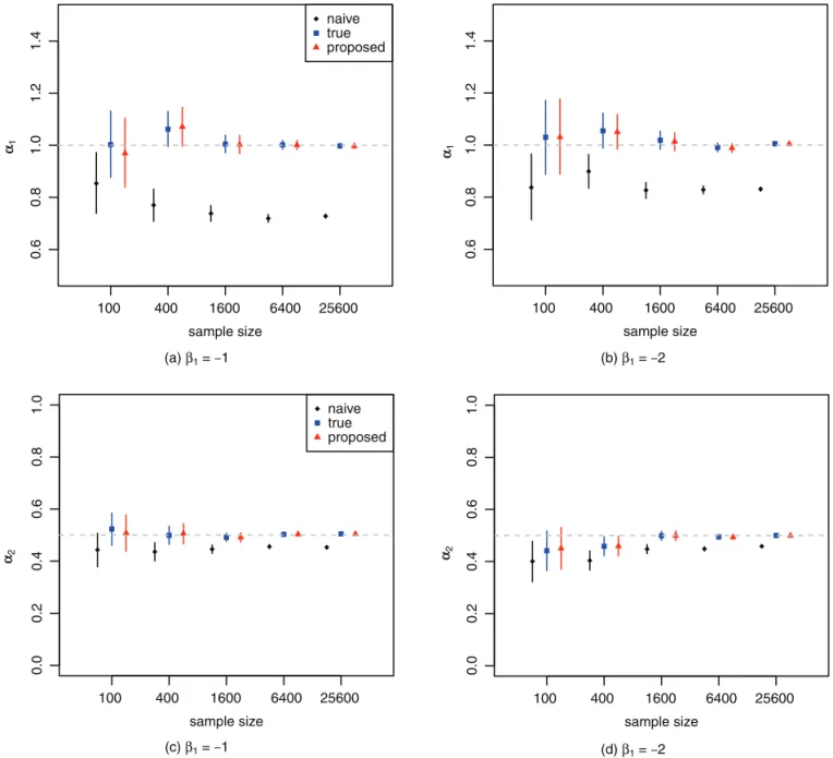
true risk status V and X, for each of the five sample sizes. The credible intervals are based on 5,000 pos­ terior samples, with an effective size over 4,500. For MCMC, an effect size close to the nominal size indi­ cates there is very little autocorrelation in the pos­ terior samples that may jeopardize the efficiency in the estimation. We observe that the naive estimates are biased downward compared to those from the true models using the corresponding values of V. That is, misrepresentation in the risk factor causes an attenu­ ation effect in the naive estimates for the risk effect

α1 for V, an effect commonly seen in measurement

error modeling. The center of the posterior distribu­ tion for the regression effect α1 from the proposed

# Prior distributions p ~ dunif(0, 1)

theta ~ dunif(0, 1) aa0 ~ dnorm(0, 0.1) aa1 ~ dnorm(0, 0.1) aa2 ~ dnorm(0, 0.1) alpha ~ dgamma(0.5, 0.5) }

Using the observed values of (y₁, v*, x_{1 1}), (y₂, v₂*, x₂),

. . . , (y_n, v*, x_n n), the above BUGS program will output

posterior samples of the parameters α0, α1, α2, p, q,

q and j. Note that the above normal and gamma prior distributions are chosen as vague priors that will work well for cases where the true parameters have values near 1, as in the simulation study. For real applications depending on the scales of the response and covariates, we may need to re­set the super­ parameters or standardize continuous covariates in order for the normal and gamma priors to cover a range reasonably larger than the scale of the param­ eters. The use of WinBUGS and OpenBUGS for actuarial modeling was illustrated in earlier papers such as Scollnik (2001, 2002). With R packages such as R2WinBUGS and BRUGS, we will be able to perform repeated computations using R.

3.2. Impact from a correctly

measured rating factor

Here, we include an additional risk factor X that is correctly measured. In the simulation study, we first generate the true risk status V, the additional factor X and the claim outcome Y from the true dis­ tributional structure for the gamma severity model in Example 2.1. The samples of V are then modified based on the true values of p in order to obtain the corresponding observed samples of V *. The pro­ posed model uses simulated samples of (Y, V *, X) to estimate the parameters in the gamma distributional structure given in Example 2.1.

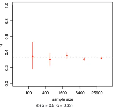
obtain the number of misrepresented cases directly from data on the reported status. The credible intervals for the misrepresentation probability p have very similar patterns, and thus will not be presented here. The credible interval becomes narrower as the sam­ ple size increases, with all the intervals covering the true value of the probability. In both figures, there is larger variability in the estimation for the case with p = 0.50, where the issue of misrepresentation is more severe.

model is very close to that from the true model. There seems to be no noticeable difference concern­ ing the estimation of α2. The proposed model seems

to give wider credible intervals, acknowledging the additional uncertainty due to the existence of the misrepresentation.

Figure 3 presents the credible intervals of the prevalence of misrepresentation q from the proposed model. For insurance applications, the prevalence q is a more meaningful measure that will allow us to

0.5

1.0

1.5

sample size

100 400 1600 6400 25600 `1

sample size `2

0.2

0.3

0.4

0.5

0.6

0.7

0.8 naive true proposed

100 400 1600 6400 25600 sample size

`2

0.2

0.3

0.4

0.5

0.6

0.7

0.8

100 400 1600 6400 25600

sample size `1

0.5

1.0

1.5

naive true proposed

100 400 1600 6400 25600 (a) p = 0.25 (b) p = 0.5

(c) p = 0.25 (d) p = 0.5

earlier for obtaining the samples of (V*, V₁ *). For all ₂ the models, independent normal priors with mean 0 and variance 10 are used for the regression coeffi­ cients. For the probability parameters q1, q2, p1 and

p₂, uniform priors on (0, 1) are used. Other MCMC details are the same as those for the gamma model.

Figure 4 presents the 95% equal­tailed credible intervals for the regression coefficients α1 and α2 of

the true risk statuses V₁ and V₂, for each of the five sample sizes. As expected, we observe that the naive estimates are biased downward to a certain extent, compared to those from the true models using the corresponding values of V₁ and V₂. That is, mis­ representation in the risk factor causes an attenua­ tion effect in the naive estimates. The centers of the posterior distributions for the regression effects α1 and

α2 from the proposed model are very close to those

from the true model, for sufficiently large sample sizes. For the negative binomial model, the pro­ posed method gives much wider credible intervals, when compared with those from a Poisson model we tried with two misrepresented risk factors. The exis­ tence of misrepresentation seems to cause a larger efficiency loss in the negative binomial model than its Poisson counterpart, owing to the weak identification

3.3. Multiple rating factors

with misrepresentation

The second case we study is when we have two rating factors that are subject to misrepresentation. For the negative binomial loss frequency model in Example 2.2, we generate samples for the five sample sizes for the true risk statuses (V₁, V₂), using two Bernoulli trials with the binomial probabilities

q1= 0.5 and q2= 0.4, respectively. Two different sets

of values of ( p₁, p₂), (0.25, 0.15) and (0.35, 0.25), are used for the two risk factors for obtaining the corresponding samples of (V₁*, V*). The correspond­₂ ing samples of negative binomial counts Y are then generated from those of V₁ and V₂, with regression coefficients (α0, α1, α2) being (−1, 1, 0.5), and a

dispersion parameter j = 5. The proposed model uses simulated samples of (Y, V*, V₁ 2*) to estimate the

parameters in the negative binomial distributional structure given in Example 2.2.

We compare the results from the proposed model in (4) with naive estimates from negative binomial regression using the observed values of (V*, V₁ *), pre­₂ tending there to be no misrepresentation. We denote the true model as negative binomial regression using the corresponding values of (V₁, V₂) that we used

Figure 3. 95% credible intervals for the prevalence of misrepresentation q for the gamma loss severity model

0.0

0.2

0.4

0.6

0.8

1.0

sample size

q

100 400 1600 6400 25600

(a) p = 0.25 (q = 0.2)

0.0

0.2

0.4

0.6

0.8

1.0

sample size

q

100 400 1600 6400 25600

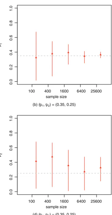
as the sample size increases, with all the intervals covering the true value of the probability. In both fig­ ures, there is larger variability in the estimation for the case with (p₁, p₂) = (0.35,0.25), where the issue of misrepresentation is more severe.

3.4. Embedded model on prevalence

of misrepresentation

The last case we study is when there is a correctly measured risk factor X that affects the prevalence of misrepresentation q. The process of data simulation (Xia and Gustafson 2016) when the dispersion

parameter is large. The results for the Poisson model have similar patterns as those in Figures 2 and 3, and are not presented here. We further observe that the model works better when the sample size increases, which suggests that it will work for large insurance claim datasets.

Figure 5 presents the credible intervals of the prob­ abilities p₁ and p₂ from the proposed model. The results on the five prevalence of misrepresentation q_j’s are similar. The credible interval becomes narrower

Figure 4. Credible intervals for the risk effects of V1 (top) and V2 (bottom) for the negative binomial

loss frequency model. The dashed line marks the true value

0.0

0.5

1.0

1.5

2.0

2.5

sample size

100 400 1600 6400 25600

0.0

0.5

1.0

1.5

2.0

2.5

sample size

100 400 1600 6400 25600

0.0

0.5

1.0

1.5

2.0

2.5

sample size

100 400 1600 6400 25600

0.0

0.5

1.0

1.5

2.0

2.5

sample size

naive true proposed

100 400 1600 6400 25600

(a) (p1, p2) = (0.25, 0.15) (b) (p1, p2) = (0.35, 0.25)

(c) (p1, p2) = (0.25, 0.15) (d) (p1, p2) = (0.35, 0.25)

`2 `1

risk status V *, using a Bernoulli trial with the prob­ ability q* = 0.5. The samples of the additional risk factor X are generated from a gamma distribution with the shape and scale parameters being 2 and 0.5, respectively. For the true model, we generate the corresponding samples of V, assuming that the pre­ valence of misrepresentation is given by logit (q) = β0 + β1X. We assume the regression coefficients

in logistic regression, (β0, β1), take two sets of

values, (0, −1) and (0, −2). For each sample of X, we calculate the prevalence of misrepresentation differs, as we need to determine the value of q for

each sample X. We directly simulate samples of V * from a Bernoulli trial with a probability q* and use them to obtain those of V based on the calculated values of q. The samples of V and X are then used to obtain those for the outcome Y. The proposed model uses simulated samples of (Y, V *, X) to estimate the parameters in the Poisson distributional structure given in Example 2.3.

We use the Poisson model in Example 2.3 to generate a single sample of size n for the reported

Figure 5. Proposed 95% credible intervals for the probabilities p1 and p2 for the negative binomial

loss frequency model

0.0

0.2

0.4

0.6

0.8

1.0

sample size

p1

100 400 1600 6400 25600

0.0

0.2

0.4

0.6

0.8

1.0

sample size

p2

100 400 1600 6400 25600

0.0

0.2

0.4

0.6

0.8

1.0

sample size p2

100 400 1600 6400 25600

0.0

0.2

0.4

0.6

0.8

1.0

sample size

p1

100 400 1600 6400 25600

(a) (p1, p2) = (0.25, 0.15) (b) (p1, p2) = (0.35, 0.25)

representation using the observed risk status V *. For all the models, independent normal priors with mean 0 and variance 10 are used for all the regres­ sion coefficients and the logarithm of the dispersion parameter. For the probability parameter q, a uniform prior on (0, 1) is used. Other MCMC details are the same as those for the gamma model.

Figure 6 presents the 95% credible intervals for the regression coefficients α1 and α2 of the true risk

status V and X, for each of the five sample sizes. For both α1 and α2, we observe that the naive estimates

and obtain the corresponding true samples of V based on those of V *. The corresponding samples of Poisson counts Y are then generated from those of V and X, with regression coefficients (α0, α1, α2)

being (1.2, 1, 0.5).

We compare the results from the proposed model with naive estimates from Poisson regression using the observed values of V *, pretending there to be no misrepresentation. We denote the true model as Poisson regression using the corresponding values of V. The proposed model is based on the mixture

0.0

0.2

0.4

0.6

0.8

1.0

sample size

naive true proposed

100 400 1600 6400 25600 `2

0.6

0.8

1.0

1.2

1.4

sample size

naive true proposed

100 400 1600 6400 25600 `1

(a)β1 = –1

(c)β1 = –1

0.0

0.2

0.4

0.6

0.8

1.0

sample size

100 400 1600 6400 25600 `2

0.6

0.8

1.0

1.2

1.4

sample size

100 400 1600 6400 25600 `1

(b)β1 = –2

(d)β1 = –2

and true models do not assume misrepresentation in the risk factor, so there is no inference for the coef­ ficient β1 from the latent model on the prevalence of

misrepresentation.

4. Case study on medical

expenditures

The Medical Expenditure Panel Survey (MEPS, AHRQ 2013) is a set of national surveys on medical expenditures and frequencies of health care utiliza­ tion by the Americans. In the actuarial and statistical literature, the MEPS data have been used by earlier papers such as Frees et al. (2013), Xia and Gustafson (2014, 2016), Hua and Xia (2014) and Hua (2015) for exploring patterns concerning health care loss frequency and severity. For the case study, we use the 2013 MEPS consolidated data to illustrate the proposed GLM loss frequency and severity models that embed a predictive analysis on the misrepresen­ tation risk.

In the case study, we choose two response variables, the office­based visits and total medical charges, respectively, for our loss frequency and severity models. According to the Patient Protection and are biased downward compared to those from the

true models using the corresponding values of V. This means misrepresentation in one risk factor may cause bias in the estimates of effects for both the risk factor itself (i.e., the attenuation effect), as well as for other risk factors. The centers of the posterior distributions for the regression effects α1 and α2 from the proposed

model are very close to those from the true model. The proposed model seems to give a little larger pos­ terior standard deviation, acknowledging the uncer­ tainty due to the existence of misrepresentation.

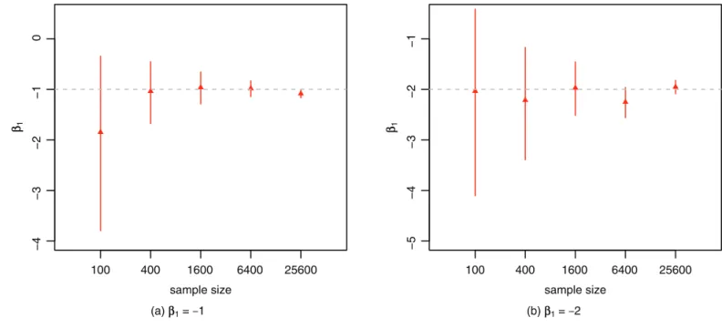
Figure 7 presents the credible intervals of the risk effect β1 on the prevalence of misrepresentation from

the proposed model. The credible interval becomes narrower as the sample size increases, with all the intervals covering the true value of the coefficient. In both figures, there is larger variability in the esti­ mation for the case with β1 = −2, where the pre­

valence of misrepresentation q varies more widely with the factor X. When compared with Figure 6, we observe that the credible intervals for the regression coefficients β1 are wider than those for α1 and α2 that

have a similar scale. This indicates that latent models may require a larger sample size to learn the param­ eters with the same precision. Note that the naive

−4

−3

−2

−1

0

sample size

100 400 1600 6400 25600

a1

−5

−4

−3

−2

−1

sample size

100 400 1600 6400 25600

a1

(a) a1 = –1 (b)a1 = –2

Figure 7. Proposed 95% credible intervals for the risk effect a1 on the prevalence of misrepresentation

Example 2.3, despite differences in the distributional form of Y. The MCMC settings are similar to those in the previous section. For the regression coeffi­ cients α0, α1, α2, β0 and β1, we specify vague nor­

mal priors with mean 0 and variance 10 (100 for the gamma model to account for a larger scale of Y ). For the probability q, we assume a beta prior with both parameters being 2 (corresponding to prior mean 0.5 and standard deviation 0.224). At the current sample sizes, the slightly more concentrate beta prior seems to help with the convergence of the negative binomial model. For the probabilities p and q, the prior distri­ butions are transformations of those for β0, β1 and q,

according to the relationships of the parameters. In Figure 8, we present the 95% equal­tailed cred­ ible intervals for the relativity exp(α1) and exp(α2)

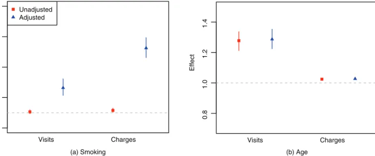
concerning the smoking and age effects on the aver­ age number of office­based visits and the average total medical charges. We observe that for the smok­ ing risk factor, the adjusted models give estimated relativities that are substantially higher than those from the unadjusted models. Note that the above dif­ ference in the estimated relativity is very large, as the relativity is the exponential of the regression coeffi­ cients. When we look at the regression coefficients, Affordable Care Act (PPACA), health insurance

premiums can account for the five risk factors of age, location, tobacco use, plan type (individual vs. family) and plan category based on the level of coverage. For the MEPS data, we choose the two factors of age and smoking status that are available in the dataset. In particular, the self­reported smok­ ing status may be subject to misrepresentation, owing to social desirability concerns. For the empirical analysis, we include insured individuals from the age of 18 to 60 who were the reference person in their household. The sample sizes for the office­based visits and the total medical charges are 3,249 and 2,948, respectively. The sample size is smaller for the total medical charges variable, as we only include individuals with a positive expenditure.

Due to the over­dispersed feature of the office­ based visits variable, we specify a negative binomial GLM for the loss frequency model. For the total medi­ cal charges variable, we use a gamma GLM for the loss severity model. We first perform an unadjusted analysis, using regular GLM ratemaking models, without adjusting for misrepresentation in the self­ reported smoking status. For the adjusted analysis, we adopt the same regression structures as those in

0

2

4

6

8

Effect

Visits Charges Unadjusted

Adjusted

(a) Smoking

0.8

1.0

1.2

1.4

Effect

Visits Charges (b) Age

Figure 8. Credible intervals for the relativity of smoking and age, exp(`1) and exp(`2), for the negative

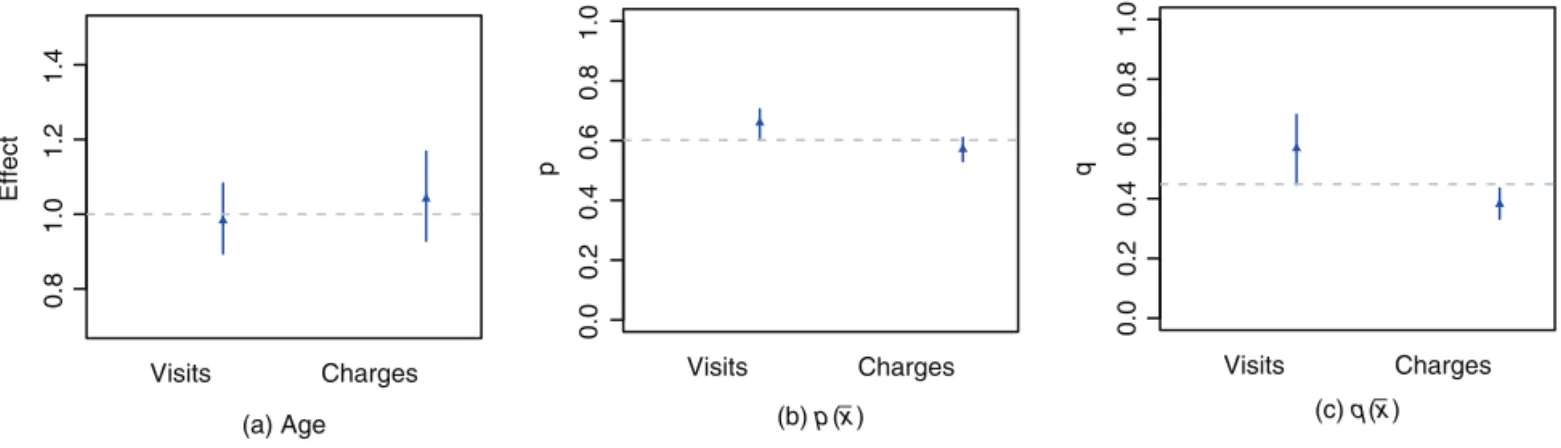
of misrepresentation (i.e., q/(1 − q)), the predicted misrepresentation probability p(x–), and the predicted prevalence of misrepresentation q(x–) for individuals at the average age of 42. We observe that the age effect is insignificant in predicting the prevalence of misrepresentation q regarding both outcomes on the office­based visits and total medical charges. For individuals at the average age, the predicted mis­ representation probabilities are 66% and 57% for office­based visits and total medical charges. The credible intervals overlap for the two models using samples on different outcomes, indicating no statisti­ cal difference in the two probabilities. The predicted prevalence of misrepresentation is about 57% and 38%, with a larger difference caused by difference in the percentage of smokers in the gamma model that excludes individuals with no medical charge. Among people with an average age who identified themselves as nonsmokers, about 48% of them are estimated to have misrepresented their smoking status.

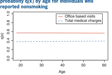
In Figure 10, we present the predicted prevalence of misrepresentation by age for individuals who iden­ tified themselves as nonsmokers. For both the office­ based visits and total medical charges, the predicted prevalence of misrepresentation does not seem to vary with age. For both models, we can predict the prevalence of misrepresentation for individuals with a specific age. For example, for respondents who the estimates are comparable to those from the

simulation studies in the previous section. With the estimated prevalence q ranging from 0.38 to 0.57, such an estimated difference is likely to be attributed to misrepresentation. From a practical standpoint, the estimated smoking relativity from the unadjusted analysis is very close to one, contradictory to clinical findings on the health risks associated with smoking. For the current study, the estimates from the adjusted model are more likely to reflect the true smoking effect on the health outcomes. In general, however, business knowledge needs to be used when interpreting results from empirical studies. In the case of observation studies, there is a possibility of heterogeneity due to confounding from other risk factors, such as exposure to secondhand smoke in the current case. In such cases, the embedded analysis help us identify heterogeneity in the data that may require inclusion of other risk fac­ tors. The predictive model on the misrepresentation risk could provide insights to the underwriting depart­ ment that would help optimize the cost/benefit tradeoff of undertaking interventions to minimize the occur­ rence of such frauds. For the age effect, the adjustment results in no noticeable difference in the estimated rela­ tivity. Both the smoking and age effects are significant from the adjusted model, confirming our intuition.

In Figure 9, we present the 95% equal­tailed cred­ ible intervals for the relative age effect on the odds

Figure 9. Adjusted credible intervals for the age effect exp(a1) on the odds of misrepresentation,

the predicted misrepresentation probability p(x–), and the prevalence of misrepresentation q(x–)

for individuals at the average age of 42. In each panel, the left column corresponds to the negative binomial model on office-based visits, and the right column corresponds to the gamma model on total medical charges

0.0

0.2

0.4

0.6

0.8

1.0

q

Visits Charges

0.0

0.2

0.4

0.6

0.8

1.0

p

Visits Charges

0.8

1.0

1.2

1.4

Effect

Visits Charges

models with concomitant variables, we embedded a predictive analysis of misrepresentation risk by a latent logistic regression model on the prevalence of misrepresentation. For insurance companies that have information on various risk factors concerning an insured policy, such an embedded model on the prevalence of misrepresentation allows the under­ writing department to generate a misrepresentation risk profile based on models fitted from historical data. Using the risk profiles, the underwriting department may choose to undertake investigations on certain policies, in order to minimize the occurrence of mis­ representation frauds. By concentrating on policies with a higher misrepresentation risk, the analysis will help enhance the efficiency of underwriting practices. For the claims department, risk profiles on misrepre­ sentation on policy applications may be further used to identify fraudulent claims.

Acknowledgments

The authors are grateful to the editor, associate editor and anonymous referees for their valuable comments and suggestions that help significantly improve the quality of the paper. The authors are grateful to the Casualty Actuarial Society (CAS) for their generous support at the 2016 Individual Grant Competition and the travel support for presenting the work at the 2016 CAS Annual Meeting. The work was funded earlier by the Research and Artistry Opportunity Grant at the Northern Illinois Univer­ sity (NIU). Last but not least, we would like to thank Lauren Anglin for her work in obtaining the observ­ able moments funded through the Student Engage­ ment Funding at NIU, and her helpful comments that helped improve the slides for the presentation at the CAS Annual Meeting.

Appendix

A.1. Additional derivation for Section 2.2

Here we derive the forms of the prevalence of mis­ representation, the q_j’s, for the model in Equation (2.4). Using Bayes’s Theorem, we have

were 60 years old, the predicted prevalence of mis­ representation is 56.6% and 38.7%, respectively, for the office­based visits and the total medical charges. It is not surprising for the predicted prevalence of mis­ representation to differ, as the percentages of smokers seem to differ in the sub­sample of individuals used for the gamma model who had positive medical charges. The predicted prevalence parameters of mis­ representation constitute risk scores concerning the misrepresentation risk. Here the age effect in Figure 9 is an insignificant risk factor concerning the mis­ representation probability, as there is no evidence that people will become more honest or less honest over time. With real insurance data, we may be able to identify other significant factors when we have a much larger sample size as well as a larger number of risk factors.

5. Conclusions

In the paper, we proposed an embedded predictive analysis of misrepresentation risk in GLM ratemaking models. Under the GLM ratemaking structure, we derived the mixture regression form for the condi­ tional distribution of the claim outcome given the observed risk factors when some of them are subject to misrepresentation. The mixture regression form ensures the model identifiability, so that all parameters including the true relativities and the prevalence of misrepresentation can be estimated consistently using regular ratemaking data. Based on mixture regression

20 30 40 50 60

0.0

0.2

0.4

0.6

0.8

1.0

Age

q(x)

Office based visits Total medical charges

Atienza, N., J. Garcia­Heras, and J. M. Munoz­Pichardo, “A New Condition for Identifiability of Finite Mixture Distributions,”

Metrika 63(2), 2006, pp. 215–221.

Bermúdez, L., and D. Karlis, “A Posteriori Ratemaking Using Bivariate Poisson Models,” Scandinavian Actuarial Journal, 2015, pp. 1–11.

Brockman, M. J., and T. S. Wright, “Statistical Motor Rating: Making Effective Use of Your Data,” Journal of the Institute

of Actuaries 119, 1992, pp. 457–543.

1, 1 * 0, * 1

* 0, * 1 1, 1 1, 1

* 0, * 1 , ,

1

0 0 1 1 1 1 1

1 1 2 1 2

1 2 1 2 1 2

1 2 1 1 2 2

0,1 ; 0,1 1 1 2 2

1 2 1 2

2 1 2 1 2 1 2

1 1 1 1 1 2

q P V V V V

P V V V V P V V

P V V V v V v P V v V v

p p

p p p

p p v v

∑

(

)

(

) (

)

(

) (

)

(

)

(

)

( )

(

)

(

)

= = = = = = = = = = = = = = = = = =

= − θ θ

+ + − − θ θ + − θ θ =

θ

− θ −

{ } { }

∈ ∈

1, 1 * 1, * 0

* 1, * 0 1, 1 1, 1

* 1, * 0 , ,

1

0 0 1 1 1 1 1

2 1 2 1 2

1 2 1 2 1 2

1 2 1 1 2 2

0,1 ; 0,1 1 1 2 2

1 2 1 2

1 1 2 1 2 1 2

2 2 2 2 1 2

q P V V V V

P V V V V P V V

P V V V v V v P V v V v

p p

p p p

p p v v

∑

(

)

(

) (

)

(

) (

)

(

)

(

)

( )

(

)

(

)

= = = = = = = = = = = = = = = = = =

= − θ θ

+ + − θ − θ + − θ θ =

θ

− θ −

{ } { }

∈ ∈

1, 1 * 0, * 0

* 0, * 0 1, 1 1, 1

* 0, * 0 , ,

1 1 1 1

3 1 2 1 2

1 2 1 2 1 2

1 2 1 1 2 2

0,1 ; 0,1 1 1 2 2

1 2 1 2

1 2 1 2 1 1 2 2 1 2 1 2 1 2

q P V V V V

P V V V V P V V

P V V V v V v P V v V v

p p

p p p p

v v

∑

(

)

(

) (

)

(

) (

)

( ) ( ) ( )( ) = = = = = = = = = = = = = = = = = =

= θ θ

θ θ + θ − θ + − θ θ + − θ − θ

{ } { }

∈ ∈

0, 1 * 0, * 0

* 0, * 0 0, 1 0, 1

* 0, * 0 , ,

1

1 1 1 1

4 1 2 1 2

1 2 1 2 1 2

1 2 1 1 2 2

0,1 ; 0,1 1 1 2 2

2 1 2

1 2 1 2 1 1 2 2 1 2 1 2 1 2

q P V V V V

P V V V V P V V

P V V V v V v P V v V v

p

p p p p

v v

∑

(

)

(

) (

)

(

) (

)

( ) ( ) ( ) ( )( ) = = = = = = = = = = = = = = = = = =

= − θ θ

θ θ + θ − θ + − θ θ + − θ − θ

{ } { }

∈ ∈

1, 0 * 0, * 0

* 0, * 0 1, 0 1, 0

* 0, * 0 , ,

1

1 1 1 1 .

5 1 2 1 2

1 2 1 2 1 2

1 2 1 1 2 2

0,1 ; 0,1 1 1 2 2

1 1 2

1 2 1 2 1 1 2 2 1 2 1 2 1 2

q P V V V V

P V V V V P V V

P V V V v V v P V v V v

p

p p p p

v v

∑

(

)

(

) (

)

(

) (

)

( ) ( ) ( ) ( )( ) = = = = = = = = = = = = = = = = = =

= θ − θ

θ θ + θ − θ + − θ θ + − θ − θ

{ } { }

∈ ∈

References

AHRQ (Agency for Healthcare Research and Quality), Medical Expenditure Panel Survey. Rockville, MD, U.S. Department of Health and Human Services, 2013.

Atienza, N., J. Garcia­Heras, J. M. Munoz­Pichardo, and R. Villa, “On the Consistency of MLE in Finite Mixture Models of Exponential Families,” Journal of Statistical Planning and

Additive Models for Location, Scale, and Shape,” Insurance:

Mathematics and Economics 55, 2014, pp. 225–249.

Lemaire, J., S. C. Park, and K. C. Wang, “The Use of Annual Mileage as a Rating Variable,” ASTIN Bulletin 46(1), 2016, pp. 39–69.

McLachlan, G., and T. Krishnan, The EM Algorithm and Exten­

sions, volume 382, Wiley, 2007.

Scollnik, D. P. M., “Actuarial Modeling with MCMC and BUGS,”

North American Actuarial Journal 5(2), 2001, pp. 96–124. Scollnik, D. P. M., “Modeling Size­of­Loss Distributions for

Exact Data in WinBUGS,” Journal of Actuarial Practice 10, 2002, pp. 202–227.

Shi, P., and E. A Valdez, “A Copula Approach to Test Asymmetric Information with Applications to Predictive Modeling,” Insur­

ance: Mathematics and Economics 49(2), 2011, pp. 226–239. Shi, P., “Insurance Ratemaking Using a Copula­Based Multi­

variate Tweedie Model,” Scandinavian Actuarial Journal 2016(3), 2016, pp. 198–215.

Liangrui Sun, Michelle Xia, Yuanyuan Tang, and Philip G. Jones. “Bayesian Adjustment for Unidirectional Misclassification in Ordinal Covariates, Journal of Statistical Computation and

Simulation 87(18), 2017, pp. 3440–3468.

Roderick S.W. Winsor, Misrepresentation and Non Disclosure

on Applications for Insurance, Blaney McMurtry LLP, 1995. Xia, M., and P. Gustafson, “Bayesian Sensitivity Analyses for

Hidden Sub­populations in Weighted Sampling,” Canadian

Journal of Statistics 42(3), 2014, pp. 436–450.

Xia, M., and P. Gustafson, “Bayesian Regression Models Adjusting for Unidirectional Covariate Misclassification,”

Canadian Journal of Statistics 44, 2016, pp. 198–218. Xia, M., and P. Gustafson, “Bayesian Inference for Unidirectional

Misclassification of a Binary Response Trait,” Statistics in

Medicine 37(6), 2018, pp. 933–947.

Yip, K. C. H., and K. K. W. Yau, “On Modeling Claim Frequency Data in General Insurance with Extra Zeros,” Insurance:

Mathematics and Economics 36(2), 2005 pp. 153–163. David, M., “Auto Insurance Premium Calculation Using Gener­

alized Linear Models,” Procedia Economics and Finance 20, 2015, pp. 147–156.

Frees, E. W., R. A. Derrig, and G. Meyers, Predictive Modeling

Applications in Actuarial Science, vol. 1, Cambridge Univer­ sity Press, 2014.

Frees, E. W., J. Xiaoli, and X. Lin, “Actuarial Applications of Multivariate Two­Part Regression Models,” Annals of Actu­

arial Science 7(2), 2013, pp. 258–287.

Bettina Grün and Friedrich Leisch, “Finite Mixtures of Gen­ eralized Linear Regression Models,” in Recent Advances in

Linear Models and Related Areas, pp. 205–230. Springer, 2008.

Grün, B., and F. Leisch, “FlexMix Version 2: Finite Mixtures with Concomitant Variables and Varying and Constant Parameters,”

Journal of Statistical Software 28, 2008, pp. 1–35.

Gustafson, P., “Bayesian Statistical Methodology for Observa­ tional Health Sciences Data,” Statistics in Action: A Canadian

Outlook, 2014, pp. 163–176.

Haberman, S., and A. E. Renshaw, “Generalized Linear Models and Actuarial Science,” The Statistician 45(4), 1996, pp. 407–436.

Hahn, P. R., J. S. Murray, and I. Manolopoulou, “A Bayesian Partial Identification Approach to Inferring the Prevalence of Accounting Misconduct,” Journal of the American Statistical

Association 111, 2016, pp. 14–26.

Hennig, C., “Identifiability of Models for Clusterwise Linear Regression,” Journal of Classification 17(2), 2000, pp. 273–296. Hua, L., and M. Xia, “Assessing High­Risk Scenarios by Full­ Range Tail Dependence Copulas,” North American Actuarial

Journal 18(3), 2014, pp. 363–378.

Hua, L., “Tail Negative Dependence and Its Applications for Aggregate Loss Modeling,” Insurance: Mathematics and

Economics 61, 2015, pp. 135–145.