Data Reduction Based on Local Hausdorff Measures for Forensic Data

Data Reduction Based on Local Hausdorff Measures for Forensic Data

Peng Tao

, Chen

Xiaoshu

, Liu Huiyu

, Chen Kai

Huazhong University of Science & Technology

Wuhan Textile University

[email protected]

doi:10.4156/jcit.vol6.issue5.31

Abstract

Currently, in many domains (e.g. multispectral images, text categorization, biometrics, retrieval of multimedia database, computer forensics), the size of the data sets is so extremely large that real-time systems cannot afford the time and storage requirements to process them. Data reduction techniques are approaches in charge of diminish the quantity of information in order to reduce both memory and execution time. In this paper, we proposed a schema to reduce the quantity of instances using local Hausdorff measures. In the schema, we divide the original data set to subsets and use the Hausdorff measures on the subsets, the instances in the set which doesn’t change or change the hausdorff distance slightly will be removed, which can reduce the quantity of the original set. The schema assures the topology of the original set and can supply a good data set for next proceeding.

Keywords

1. Introduction

Data reduction techniques are approaches in charge of diminish the quantity of information in order to reduce both memory and execution time. Traditionally, the concept of data reduction have received several names: e.g. editing, condensing, filtering, thinning, etc, depending on the objective of the data reduction task. There are two different possibilities depending on the object of the reduction. The first one is to reduce the quantity of instances, while the second one is to select a subset of features from available ones. The later, feature selection, is not considered in this paper, but just the former: prototype selection.

The term network forensics was introduced by the computer security expert Marcus Ranum in the early 90’s [1], and is borrowed from the legal and criminology fields where “forensics” pertains to the investigation of crimes. According to Simson Garfinkel, network forensic systems can be implemented in two ways: “catch it as you can” and “stop look and listen” systems [2].

Most network forensic systems are based on audit trails. Systems relying on audit trails try to detect known attack patterns, deviations from normal behavior, or security policy violations. They also try to reduce large volumes of audit data to small volumes for interesting data. One of the main problems with these systems is the overhead, which can become unacceptably high. To analyze logs, the system must keep information regarding all the actions performed, which invariably results in huge amounts of data, requiring disk space and CPU resources. Next, the logs must be processed to convert them into a manageable format, and then compared with the set of recognized misuse and attack patterns to identify possible security violations. Further, the stored patterns need to be continually updated, which would normally involve human expertise. An intelligent, adaptable and cost-effective tool that is capable of this is the goal of the researchers in cyber forensics.

2. Related Works

The many existing proposals in relation to reduce data can be categorized into two main groups. First, the schemes that merely select a subset of the original instances, Hart’s algorithm [3] represent the first reduction for the 1-NN rule. In this initial approximation, the idea of reducing with respect to the training set is used. The weakness of the hart’s method lies in the impossibility of judging whether the resulting reduced set is the smallest set. Chen & Jozwik[4] proposed a simple reduce schema which allows one to control the resulting condensed set size; the schema defined the diameter of a

training, the strategy relies on dividing the initial training set into successive subsets which are defined based on the notion diameter. This process is repeated until the number of subsets reaches the number previously established as the reduced set size. Sanchez introduced the family of RSP(Reduction by Space Partition) algorithms[5], which are based on the idea Chen’s algorithm. The Main difference between the Chen’s and one of the RSP approaches, RSP3, is that in the former, any subset containing a mixture of instances belonging to different classes can be chosen to divided. There also some other researches about the data reduction [11~13].

3. Hausdorff measures and KDD CUP’99 Data Set

3.1. KDD CUP’ 99 Data Set

In 1998, the United States Defense Advanced Research Projects Agency (DARPA)funded an “Intrusion Detection Evaluation Program (IDEP)” administered by the Lincoln Laboratory at the Massachusetts Institute of Technology. The goal of this program was to build a data set that would help evaluate different intrusion detection systems (IDS) in order to assess their strengths and weaknesses. The objective was to survey and evaluate research in the field of intrusion detection. The computer network topology employed for the IDEP program involved two sub networks: an “inside” network consisting of victim machines and an “outside” network consisting of simulated real-world Internet traffic. The victim machines ran Linux, SunOSTM, and SolarisTM operating systems. Seven weeks of training data and two weeks of testing data were collected. Testing data contained a total of 38 attacks, 14 of which did not exist in the training data. This was done to facilitate the evaluation of potential IDSs with respect to their anomaly detection performance. Three kinds of data was collected: transmission control protocol (TCP) packets using the “tcpdump” utility, basic security module (BSM) audit records using the Sun SolarisTM BSM utility, and system file dumps. This data set is popularly known as DARPA 1998 data set [6].

One of the participants in the 1998 DARPA IDEP [7], used only TCP packets to build a processed version of the DARPA 1998 data set [3]. This data set, named in the literature as KDD intrusion detection data set [8], was used for the 1999 KDD Cup competition [9], which allowed participants to employ it for developing IDSs. Both training and testing data subsets cover four major attack ategories: Probing (information gathering attacks), Denial-of-Service (deny legitimate requests to a system), User-to-Root (unauthorized access to local super-user or root), and Remote-to-Local (unauthorized local access from a remote machine). Each record consists of 41 features [10], where 38 are numeric and 3 are symbolic, defined to characterize individual TCP sessions.

3.2. Hausdorff Measures

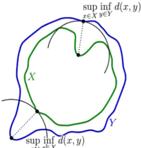
In mathematics, the Hausdorff distance, or Hausdorff metric, measures how far two subsets of a metric space are from each other. It turns the set of non-empty compact subsets of a metric space into a metric space in its own right. It is named after Felix Hausdorff.

Informally, two sets are close in the Hausdorff distance if every point of either set is close to some point of the other set. The Hausdorff distance is the longest distance you can be forced to travel by an adversary who chooses a point in one of the two sets, from where you then must travel to the other set.

Let X and Y be two non-empty subsets of a metric space (M, d). We define their Hausdorff distance d H(X, Y) by

(1)

Where sup represents the supremum and inf the infimum. d(x, y) denotes the euclidean distance between x and y. The properties of the Hausdorff distance as follows:

(1) In general may be infinite. If both X and Y are bounded, then is guaranteed to be finite;

(2) We have =0 if and only if X and Y have the same closure;

(3) On the set of all non-empty subsets of M, dH yields an extended pseudometric.

(4) On the set F(M) of all non-empty compact subsets of M, dH is a metric. If M is complete, then so

is F(M). If M is compact, then so is F(M). The topology of F(M) depends only on the topology of M, not on the metric d.

The geometry description of Hausdorff Distance can be shown in fig 1:

Figure 1. Components of the calculation of the Hausdorff distance between the green line X and the blue line Y.

The definition of the Hausdorff distance can be derived by a series of natural extensions of the distance function d(x, y) in the underlying metric space M, as follows:

(1) Define a distance function between any point x of M and any non-empty set Y of M by: (2)

(2) For example, d(1, [3,6]) = 2 and d(7, [3,6]) = 1.

(3) Define a distance function between any two non-empty sets X and Y of M by: (4)

(3) (5) For example, d([1,7], [3,6]) = d(1, [3,6]) = 2.

(6) If X and Y are compact then d(X,Y) will be finite; d(X,X)=0; and d inherits the triangle inequality property from the distance function in M. As it stands, d(X,Y) is not a metric because d(X,Y) is not always symmetric, and d(X,Y) = 0 does not imply that X = Y (It does imply that ). For example, d([1,3,6,7], [3,6]) = 2, but d([3,6], [1,3,6,7]) = 0. However, we can create a metric by defining the Hausdorff distance to be:

4. Data Reduction Algorithm Based on Hausdorff Distance

The schema of data reduction has proposed were destroyed the topology of the original dataset, which will reduce the classification accuracy. In order to maintain the topology of the original dataset, Hausdorff Distance is used.

4.1. Local Hausdorff Distance Algorithm

In section III, we can get that, the Hausdorff Distance( ) can be used to measure the similarity of two sets. The smaller of two set, the similarity of them is higher. The data reduction based on Hausdorff Distance can be described as:

Algorithm 1: Pseudo-code for Local dataset Original data set X.

ArrayDh[k]; ArrayZero[k/2]; For x X, S=k-NN(x); For y S S’ = S-y; ArrayDh [i]=dH(S,S’); If(ArrayDh [i]> ) Add(y) to B; If(ArrayDh [i]==0) Flag=Find(y, ArrayZero); If(!Flag) Add(y) to B: Add(y) to ArrayZero; End if End if End for Add(ArrayZero) to B; X=X-S; End for

For instance x X, X is the original dataset, and the k nearest neighbor of x is gotten, which

combined the local sub set S, for very instance y S, S’=S-y, the Hausdorff distance (Hd) of S and S’ is computed:

(1) if Hd< ( is the threshold), means that the instance y doesn’t affect the topology of data set S, so, y can be removed from S, otherwise, y cannot be removed from S.

(2) if Hd=0; which means that, there at least exist a instance have the same location with y or almost the same location with y, y should remain in S, and other instance(s) can be removed from S;

1.51 1.515 1.52 1.525 1.53 1.535 12 13 14 15 2.5 3 3.5 4

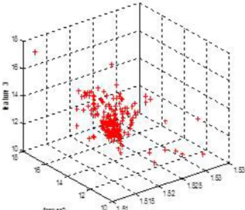
We use UCI machine learning database repository to test our algorithm. The Glass dataset is chosen, in the Glass Identification database there are 214 instance that represent 6 different types of glass(defined in terms of their oxide content:Na, Fe, K,etc). Each class is represented by 70,76,17,13,9 and 29 examples respectively. It has 9 numeric-valued features, and it comes from the USA Forensic Science Service. There features are chosen, figure 1 is the Representation of the Glass:

In Figure 2 is the subset of Glass which includes 30 instance, symbol ‘+’ in figure 2 is the instances that make the Hausdorff distance to zero, the symbol ‘o’ is the instance that make the max Hausdorff distance. From figure 2, we can get that, the instance of max Hausdorff distance is the instance that will affect the topology of the set. The larger Hausdorff distance, the more effect of topology. So we remove some instances which Hausdorff distance is smaller than threshold , the

figure 3 is the reduced subset with =0.06 and the reduction rate is 40%.

4.2. Data Reduction for KDD CUP’ 99 Data Set

In section 3, we know that each record of the Data set consists of 41 features where 38 are numeric and 3 are symbolic, at the same time, the dimension of each features are different. For example, the follow is a normal record: 0,tcp,http,SF,181,5450,0,0,0,0,0, 1,0,0,0,0, 0,0,0,0,0,0,8, 8,0.0,0,0.00,0.00,0.00,1.00,0.00,0.00,9,9,1.00,0.00,0.11,0.00,0.00,0.00,0.00,0.00.

Fig 1. Representation of the Glass Fig 2. Max Hd and min Hd of Sub set in Glass

Fig 3. Remove some instance from Subset in Glass

The first feature is “Length (# of seconds) of the connection”, the fifth feature is “data bytes from source to destination”, the seventh feature is a flag that “1 if connection is from/to the same host/port;

0 otherwise”. In order to find the attack data in the data set, we should apply the clustering algorithm on the data set. Before clustering, we must pre-process the data set:

4.2.1. Replacing the Symbolic with Numeric

The feature 2(Type of the protocol, e.g. tcp, udp, etc.), feature 3(Network service on the destination, e.g., http, telnet, etc.), feature 4(Normal or error status of the connection) features of the record are symbolic, there are three type of the protocol, 66 type of network service and 11 type of status in the data set. A simple way is used to replace the symbolic, 1 replace “tcp”, 2 replace “udp” and 3 replace “icmp”.do the same work for next 2 features. So we get the numerical record: 0,1,21,10,181,5450,

0,0,0,0,0,1,0,0,0,0,0,0,0,0,0,0,8,8,0.00,0.00,0.00,0.00,1.00,0.00,0.00,9,9,1.00,0.00,0.11,0.00,0.00,0.00 ,0.00,0.00.

4.2.2. Standardizing the Data Set

In the data set, the value of sixth features is much larger than the value of the second feature, which will affect the clustering, so we should eliminate the effect of the dimension.

(k)=

Formula (4) is a way to standardize the data set, which make the average is zero and the variance is one. With the formula(4), we can get the record:

-0.0354,-0.7746,0.7746,0,-0.3502,0.5836,0,0,0,-0.0614,0,0.7746,0,-0.0354,0,0,0,0,0,0,0,0,-0.8880,-0. 9775,-0.0772,-0.0765,0,0,0,0,-0.3165,-1.3338,-28.2666,0,0,-0.5937,-0.4939,-0.1131,-0.2107. 4.2.3 Reduce the KDD CUP99 Data set

With the previous works, we can get the algorithm of data reduction. The algorithm described as follow:

Algorithm 2: Data reduction for KDD CUP 99

Input: Dataset S n×D, number of neighbors K, Threshold Output: Dataset of reduction Y.

Step 1: replaces the symbolic with numeric in Dataset S; Step 2: standardizing the Dataset S with formula (5); Step 3: applying the algorithm 1 on dataset S; 4 Algorithm complexities

The algorithm complexity of data reduction including the complexity of K nearest neighbors (O (n)), complexity of Hausdorff distance (O(n2));

The storage consume including: Original Dataset (N*D), Reduction dataset (N’*D) and the temporary dataset K*D*2, so, the total storage consume is D*(N+N’+2*K), the N is the number of instances in original dataset and the N’ is the number of instances in Reduction dataset.

5. Experiments Result and Future Work

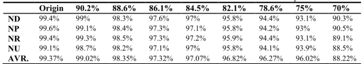
In order to test the validity of the reduction, the clustering algorithm is used to analyze the original data set and the reduction dataset. We extract part records of DoS,PROBE,R2L,U2R and NORMAL in the data set from original dataset randomly, 5 test dataset were gotten, namely, NORMAL and DoS(ND), NORMAL and PROBE(NP), NORMAL and R2L,(NR) NORMAL and U2R(NU), DoS,PROBE,R2L,U2R and NORMAL, each dataset contain 11204 records.

Table 1. Reduction Rate and the effect of classification accuracy Origin 90.2% 88.6% 86.1% 84.5% 82.1% 78.6% 75% 70% ND 99.4% 99% 98.3% 97.6% 97% 95.8% 94.4% 93.1% 90.3% NP 99.6% 99.1% 98.4% 97.3% 97.1% 95.8% 94.2% 93% 90.5% NR 99.4% 99.3% 98.5% 97.3% 97.2% 95.9% 94.4% 93.1% 89.1% NU 99.1% 98.7% 98.2% 97.1% 97% 95.8% 94.1% 93.9% 88.5% AVR. 99.37% 99.02% 98.35% 97.32% 97.07% 96.82% 96.27% 96.02% 88.22%

In table 1, we can get that, with the increase of reduction, the classification accuracy is decreasing. The tradeoff of reduction rate and the classification accuracy can be gotten from the table1. When the reduction rate increases from 10% to 15%, the decreasing of classification accuracy is small. When the reduction rate is up to 15%, the classification accuracy will decrease greatly.

This paper proposed a way to reduce the data set using local Hausdorff distance, which can maintain the geometrical distribution of original dataset. The schema can supply a good tradeoff between the reduction rate and the classification accuracy.

At the same time, there is lot of room for improvement. One could take a closer look at the effects of the parameter sets. It would be useful to find a way to get the pretty parameter for the threshold to remove the instance from original data set.

6. Reference

[1] Marcus Ranum, Network Flight Recorder. http://www.ranum.com/

[2] Simson Garfinkel, Web Security, Privacy & Commerce, 2nd Edition. http://www.oreillynet.com /pub/a/network /2002/04/26/nettap.html

[3] P.E.Hart, The Condensed Nearest Neighbor Rule, IEEE Tans. On Infromation Theory 14 no.5 (1968)505-616

[4] C.H. Chen and A.Jozwik, A Simple Set Condensation Algorithm for the Class Sensitive Artifical Neural Network, Pattern Recognition Letters. 17(1996)819-823

[5] J.S.Sanchez, High Training Set Size Reduction by Space Partitioning and Prototype Abstraction, Pattern Recogniton 37,no 7(2004) 1561-1564

[6] DARPA 1998 data set, http://www.ll.mit. edu /IST/ideval/data/1998/1998_data_index. html, cited August 2003.

[7] W. Lee, S. J. Stolfo, and K. W. Mok, A Data Mining Framework for Building Intrusion Detection Models, IEEE Symposium on Security and Privacy, Oakland, California (1999), 120-132. [8] KDD 1999 data set, http://kdd.ics.uci.edu/databases/ kddcup99/ kddcup99.html, cited August

2003.

[9] I. Levin, KDD-99 Classifier Learning Contest LLSoft’s Results Overview, ACM SIGKDD Explorations 1(2) (2000), 67-75.

[10] Tenenbaum, J. B., de Silva, V., & Langford, J. C. (2000) A global geometric framework for nonlinear dimensionality reduction, Science, 290, pp. 2319–2323.

[11] Dimensionality Reduction for Association Rule Mining, B Nath, D K Bhattacharyya, A Ghosh, International Journal of Intelligent Information Processing, Vol. 2, No. 1, pp. 9 ~ 21, 2011 [12] A Dimension Reduction Approach Using Shrinking for Multi-Dimensional Data Analysis, Yong

Shi, International Journal of Intelligent Information Processing, Vol. 1, No. 2, pp. 86 ~ 98, 2010 [13] A Feature Selection Algorithm Based on Tolerant Granule, Shifei Ding, Yu Zhang, Li Xu, Jun