Accounting for Changes in Between-Group Inequality
⇤
Ariel Burstein
UCLA
Eduardo Morales
Princeton University
Jonathan Vogel
Columbia University
June 3, 2015
Abstract
We offer a quantitative analysis of changes in U.S. between-group inequality from 1984 to 2003. We use an assignment framework with many labor groups, equipment types, and occupations in which changes in inequality are driven by shocks to work-force composition, occupation demand, computerization, and labor productivity. We parameterize our model using detailed data including direct measures of computer usage within labor group-occupation pairs. We separately quantify the impact of each shock for various measures of between-group inequality. We find, for instance, that the combination of computerization and shifts in occupation demand—which are measured without directly using data on changes in wages—account for roughly 80% and that computerization alone accounts for roughly 60% of the rise in the skill premium. We show theoretically how to link the strength of computerization and changes in occupation demand to changes in the extent of international trade.
1 Introduction
The last few decades in the United States have witnessed pronounced changes in rel-ative average wages across groups of workers with different observable characteristics (between-group inequality); see, e.g. Acemoglu and Autor (2011). For example, the wages of more educated relative to less educated workers and of women relative to men have increased substantially.1
⇤We thank Treb Allen, Costas Arkolakis, David Autor, Gadi Barlevy, Lorenzo Caliendo, Davin Chor, Arnaud Costinot, Jonathan Eaton, Pablo Fajgelbaum, Gene Grossman, David Lagakos, Bernard Salanié, Nancy Stokey, and Mike Waugh for helpful comments and David Autor and David Dorn for making their code available. Vogel thanks the Princeton International Economics Section for their support.
1The relative importance of between- and within-group inequality is an area of active research.Autor
A voluminous literature has emerged—followingKatz and Murphy(1992)—studying how changes in relative supply and demand for labor groups shape their relative wages. Changes in relative demand across labor groups have been linked prominently to com-puterization (or a reduction in the price of equipment more generally)—see e.g. Krusell et al.(2000),Acemoglu(2002a),Autor and Dorn(2013), andBeaudry and Lewis(2014)— and changes in relative demand (or productivity) across occupations or sectors, driven by structural transformation, offshoring, and international trade—see e.g. Berman et al. (1994), Autor et al. (2003), Buera et al.(2015), and Galle et al.(2015). Related to the first
1984 1989 1993 1997 2003
All 27.4 40.1 49.8 53.3 57.8
Gender Female 32.8 47.6 57.3 61.3 65.1
Male 23.6 34.5 43.9 47.0 52.1
Education College degree 45.5 62.5 73.4 79.8 85.7
No college degree 22.1 32.7 41.0 43.7 45.3
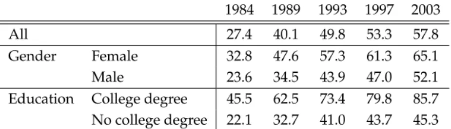
Table 1: Share of hours worked with computers
hypothesis, Table 1 shows that between 1984 and 2003 computer use rose dramatically and that computers are used more intensively by educated workers and women.2 Re-lated to the second hypothesis, Figure1shows that over the same time period education-and female-intensive occupations grew relatively quickly; see Table10in AppendixAfor details.
Figure 1: Growth (1984-2003) of the occupation share of labor payments and the average (1984 & 2003) of the share of workers in the occupation who have a college degree (left) and are female (right)
between 1980 and 2005 is proximately accounted for by the increased premium associated with schooling in general and postsecondary education in particular.” On the other hand,Helpman et al.(2012) conclude: “Residual wage inequality is at least as important as worker observables in explaining the overall level and growth of wage inequality in Brazil from 1986-1995.”
The goal of our paper is to provide a quantitative evaluation of the sources of changes in between-group inequality in the United States. We base our analysis on an assign-ment model with many groups of workers and many occupations—building on Eaton and Kortum (2002), Lagakos and Waugh (2013), and Hsieh et al. (2013)—which we ex-tend to incorporate many types of equipment. In order to shed light on the importance of classes of mechanisms through which changes in the economic environment lead to changes in relative wages across labor groups, our model incorporates shocks to (i) the
composition of labor supply across groups, (ii) a composite of occupation demand and
productivity, which we refer to as “occupation shifters,” (iii) a composite of equipment
cost and productivity, which we refer to as “equipment productivity,” and(iv)a residual
composite of other factors affecting the relative productivity of labor groups, independent of the equipment they use and occupations in which they are employed, which we refer to as “labor productivity.”3 The model’s aggregate implications for relative wages nest those of workhorse macro models of between-group inequality, e.g. Katz and Murphy (1992) andKrusell et al.(2000). In spite of its high dimensionality—in our baseline empir-ics we use 30 education-gender-age groups, 2 types of equipment, and 30 occupations— we parametrize and estimate the model in a transparent manner and perform aggregate counterfactuals to quantify the impact on between-group inequality of these four shocks. In our model, the impact of changes in the economic environment on between-group inequality is shaped by comparative advantage between labor groups, equipment types, and occupations. Consider, for example, the potential impact of computerization on a labor group—such as educated workers or women—that uses computers intensively. A labor group may use computers intensively for two reasons. First, it may have a compara-tive advantage with computers, in which case this group would use computers relacompara-tively more within occupations, as we show is the case in the data for more educated work-ers. Computerization increases the relative wage of such groups. Second, a labor group may have a comparative advantage in the occupations in which computers have a com-parative advantage, in which case this group would be allocated disproportionately to occupations in which all workers are relatively more likely to use computers, as we show is the case in the data for women. Depending on the value of the elasticity of substitution between occupations, computerization may increase or decrease relative wages of such groups and may increase or decrease employment in computer-intensive occupations.4 3These factors include, for example, discrimination and the quality of education and health systems;
see e.g.Card and Krueger(1992) andGoldin and Katz(2002).
4Our model is flexible enough so that computerization may increase the relative wage of workers who
are relatively productive using computers and may reduce the relative wage of workers employed in occu-pations in which computers are particularly productive, as described by, e.g.,Autor et al.(1998) andAutor
Therefore, measuring comparative advantage between labor groups, equipment types, and occupations is a key ingredient in our quantitative analysis.
Comparative advantage can be inferred directly from data on the allocation of workers to equipment type-occupation pairs. Changes in equipment productivity can be inferred from changes in the allocation of workers to computers within labor group-occupation pairs; controlling for labor group-occupation pairs is important because aggregate com-puter usage rises if labor groups that have a comparative advantage using comcom-puters grow or if occupations that have a comparative advantage with computers grow. Changes in occupation shifters can be inferred from changes in the allocation of workers to occu-pations within labor group-equipment type pairs, changes in labor income shares across occupations, and model parameters. Finally, changes in labor productivity can be inferred as a residual to match changes in observed average wages across labor groups.
Our procedure crucially requires information over time on the allocation of labor groups across equipment type-occupation pairs. We obtain this information for the U.S. from the October Current Population Survey (CPS) Computer Use Supplement, which provides data for five years (1984, 1989, 1993, 1999, and 2003) on whether or not a worker has direct or hands on use of a computer at work—be it a personal computer, laptop, mini computer, or mainframe—in addition to information on worker characteristics, hours worked, and occupation; see, e.g., Krueger (1993) and Autor et al. (1998) for previous studies using the October Supplement. This data is not without limitations: it imposes a narrow view of computerization that does not capture, e.g., automation of assembly lines; it only provides information on the allocation of workers to one type of equipment, com-puters; it does not detail the share of each worker’s time at work spent using comcom-puters; and it does not extend beyond 2003.5
We find that computerization alone accounts for roughly 60% of the forces that in-crease the skill premium between 1984 and 2003 and plays a similar role in explain-ing disaggregated measures of between-education inequality (e.g., the relative wage of workers with graduate training relative to high school dropouts). This result from our model is driven by the following three observations in the data. First, within labor group-occupation pairs we observe a large rise in the share of workers using computers, which our model interprets as a large increase in computer productivity (i.e. computerization). Second, more educated workers use computers relatively more within occupations than less educated workers, which—together with computerization—yields a rise in their
rel-et al. (2003).
5Our sample period, 1984-2003, accounts for a substantial share of the increase in the skill premium and
ative wages according to our model. Third, more educated workers are also dispropor-tionately employed in occupations in which all workers use computers relatively inten-sively, which—together with computerization and an estimated elasticity of substitution between occupations greater than one—also yields a rise in their relative wages accord-ing to our model. The combination of computerization and occupation shifters account for roughly 80% of the rise in the skill premium, leaving 20% to be explained by labor productivity, the shock measured to match changes in relative wages.
We find that computerization, occupation shifters, and labor productivity all play im-portant roles in accounting for the reduction in the gender gap. Computerization con-tracts the gender gap in spite of the fact that, unlike educated workers, women do not have a comparative advantage using computers because, like educated workers, women are disproportionately employed in occupations in which all workers use computers in-tensively.
Whereas in our baseline model we treat computerization and occupation shifters as changes in exogenous parameters, in Section6we take a first theoretical step to link these mechanisms to more primitive shocks. Specifically, we extend our model to incorporate international trade in equipment and sector output as well as occupation offshoring. We show that the procedure to quantify the impact on relative wages of moving to autarky is equivalent to the procedure to calculate changes in relative wages in a closed economy in which shocks are simple functions of import and export shares in the open economy. We also provide a simple procedure to quantify the differential effects on wages in a given country of changes in primitives (i.e. worldwide technologies, labor compositions, and trade costs) between two time periods relative to the effects of the same changes in primitives if that country were a closed economy.
We now discuss our contribution relative to a number of related papers in a large lit-erature. In using an assignment model of the labor market parameterized with a Fréchet distribution we follow Hsieh et al. (2013) and Lagakos and Waugh (2013). Relative to Hsieh et al.(2013), we integrate three sources of comparative advantage (between work-ers, occupations, and equipment) to quantify the role of computerization for between-group inequality.
In linking the evolution of between-group inequality to observables, rather than ex-plaining patterns in the skill premium and gender gap through latent skill- or gender-biased technological change, our paper’s objective is most similar toKrusell et al.(2000) andLee and Wolpin(2010). Krusell et al.(2000) estimate an aggregate production function which permits capital-skill complementarity and show that changes in aggregate stocks of equipment, skilled labor, and unskilled labor can account for much of the variation in
the U.S. skill premium. Whereas they identify the degree of capital-skill complementarity using aggregate time series data, we measure comparative advantage using direct mea-sures of computer allocation within labor group-occupation pairs. We also incorporate occupation shifters. Lee and Wolpin (2010) use a model of endogenous human capital accumulation in a dynamic framework to study the evolution of relative wages and labor supply and find that skill-biased technical change (the residual) plays the central role in explaining changes in the skill premium. By allowing for a greater degree of disaggre-gation (e.g. 30 occupations) and exploiting detailed data on factor allocation we reduce substantially the role of changes in the residual (labor productivity) in shaping changes in the skill premium. On the other hand, in contrast to Lee and Wolpin(2010) we treat labor composition as exogenous, measuring it in each period directly from the data.6
Two important related papers use differential regional exposure to computerization to study the differential effect across regions of technical change on the polarization of U.S. employment and wages, Autor and Dorn(2013), and on the gender gap and skill premium, Beaudry and Lewis(2014). Our approach complements these papers, embed-ding computerization into a general equilibrium model allowing us to quantify the effect of computerization (as well as other shocks) on changes over time in between-group in-equality. Instead of relying on regional variation in the exposure to computerization, we make use of detailed data on computer usage within labor group-occupation pairs.
Our focus on occupation shifters is related to a broad literature using shift-share anal-yses. For instance, Autor et al.(2003) use a shift-share analysis and find that occupation shifters account for more than 50% of the relative demand shift favoring college labor between 1970 and 1988; we arrive at a similar result using a shift-share analysis between 1984 and 2003 even though occupation shifters account for only 19% of the rise in the rel-ative wage of college labor. Under some assumptions (Cobb-Douglas utility and produc-tion funcproduc-tions), shift-share analyses structurally decompose changes in wage bill shares, i.e. changes in labor income for one labor group relative to the sum of labor payments across all labor groups, into within and between occupation shifters. However, changes in wage bill shares can be very different from changes in relative wages (on which we focus), especially when changes in labor composition are large, as they are in the data.7
6Extending our model using standard assumptions to endogenize education and labor participation
would give rise to the same equilibrium equations determining factor allocations and wages, given labor composition. Hence, our measures of shocks—to occupation shifters, equipment productivity, and labor productivity—and our estimates of model parameters would remain unchanged. In our counterfactual exercises, we fix labor composition to isolate the direct effect of individual shocks to occupation shifters, equipment productivity, and labor productivity on labor demand and wages.
7Firpo et al.(2011) uses a statistical model of wage setting to investigate the contribution of changes in
In modeling international trade in equipment, sectoral output, and occupations (e.g. offshoring) we operationalize the theoretical insights of Costinot and Vogel (2010) and Costinot and Vogel(Forthcoming) regarding the impact of international trade on inequal-ity in a high-dimensional environment. We show, as in concurrent work by Galle et al. (2015), that one can use a similar approach to that introduced byDekle et al. (2008) in a single-factor trade model—i.e. replacing a large number of unknown parameters with ob-servable allocations in an initial equilibrium—in closed and open-economy many-factor assignment models to quantify the impact of various shocks on relative wages;Burstein et al.(2013), Parro(2013), andCostinot and Rodriguez-Clare(2014) use similar approaches in models with two labor groups.
Our paper is organized as follows. We describe our framework, characterize its equi-librium, and discuss its mechanisms in Section2. We parameterize the model in Section 3, describe our baseline closed-economy results in Section4, and consider various robust-ness exercises and sensitivity analyses in Section 5. Finally, we briefly discuss how we extend the model to incorporate sectors and international trade in Section6and conclude in Section7. Many details and robustness exercises are relegated to the appendix.
2 Model
In this section we introduce the baseline version of our model, characterize the equi-librium, and show how to decompose observed changes in relative average wages be-tween any two periods into four changes in the economic environment: labor composi-tion, equipment productivity, occupation shifters and a residual that we define as labor productivity. Finally, we provide intuition for how each of these changes affects relative wages.
2.1 Environment
At timetthere is a continuum of workers indexed byz 2 Zt, each of whom inelastically supplies one unit of labor. We divide workers into a finite number of groups, indexed by
l. The set of workers in grouplis given byZt(l)✓Zt, which has massLt(l). There is a finite number of equipment types, indexed byk. Workers and equipment are employed
by production units to produce a finite number of occupations, indexed byw.8
the labor market wide returns to general skills. Our paper complements theirs by incorporating general equilibrium effects and explicitly modeling the endogenous allocation of factors.
8In order to take into consideration the accumulation of occupation-specific human capital as studied
Occupations are used to produce a single final good according to a constant elasticity of substitution (CES) production function
Yt =
Â
wµt(w)1/rYt(w)(r 1)/r
!r/(r 1)
, (1)
wherer >0 is the elasticity of substitution across occupations,Yt(w) 0 is the endoge-nous output of occupation w, andµt(w) 0 is an exogenous demand shifter for occu-pation w.9 The final good is used to produce consumption,Ct, and equipment,Yt(k),10 according to the resource constraint
Yt =Ct+
Â
kpt(k)Yt(k), (2)
wherept(k)denotes the cost of a unit of equipmentkin terms of units of the final good.11 Occupation output is produced by perfectly competitive production units. A unit hiring k units of equipment type k and l efficiency units of labor group l produces
ka[T
t(l,k,w)l]1 a units of output, where a denotes the output elasticity of equipment in each occupation andTt(l,k,w)denotes the productivity of an efficiency unit of group
l’s labor in occupation w when using equipmentk.12 Comparative advantage between
labor and equipment is defined as follows: l0 has a comparative advantage (relative
to l) using equipment k0 (relative to k) in occupation w if Tt(l0,k0,w)/Tt(l0,k,w)
have to include occupational experience as a worker characteristic when defining labor groups in the data (unfortunately, the October CPS does not contain this information) and we would have to model dynamic worker optimization. We leave these considerations for future work.
9We show in Section6 that we can disaggregateµt(w) further into sector shifters and within-sector
occupation shifters. We also show how changes in the extent of international trade/offshoring in sectoral output and occupation output generate endogenous changes in these sector shifters and a within-sector occupation shifters. For now, however, we combine sector and within-sector occupation shifters and treat them as exogenous.
10We assume that the sets of equipment types and occupations (as well as labor groups) are disjoint.
Hence, the domain of a function such asYt(·)may be the union of these sets.
11Here we have assumed that equipment fully depreciates every period. Alternatively, we could assume
thatYt(k) denotes investment in capital equipmentk, which depreciates at a given rate. All our results hold comparing across two balanced growth paths in which the real interest rate and the growth rate of relative productivity are both constant over time. We show in Section 6 how changes in the extent of international trade in equipment generates endogenous changes inpt(k). For now, however, we treat the
cost of producing equipment as exogenous.
12We restrictato be common acrossw because we do not have the data to assign a different value of
a(w)to eachw. Moreover, without affecting any of our results we can extend the model to incorporate a composite input s, which is produced linearly using the final good and which enters the production function multiplicatively ass1 h⇣ka[T
t(l,k,w)l]1 a ⌘h
. In either case,ais the share of equipment relative to the combination of equipment and labor.
Tt(l,k0,w)/Tt(l,k,w). Labor-occupation and equipment-occupation comparative ad-vantage are defined symmetrically.
A workerz 2 Zt(l)supplies#(z,k,w)efficiency units of labor if teamed with equip-mentkin occupationw. For each workerz 2Zt(l), each element of the vector#—which
contains one #(z,k,w)for each (k,w) pair—is drawn independently from a Fréchet
dis-tribution with cumulative disdis-tribution functionG(#) = exp # q , where a higher value
ofq >1 decreases the dispersion of efficiency units across(k,w)pairs.13 The assumption
that efficiency units are distributed Fréchet is made for analytical tractability; it implies that the average wage of a labor group is a CES function of prices and productivities.14
Total output of occupation w, Yt(w), is the sum of output across all units producing occupationw using any labor group land equipment type k. All markets are perfectly
competitive and all factors are freely mobile across occupations and equipment types.
Relation to alternative frameworks. Whereas our framework imposes strong restrictions on occupation production functions, its aggregate implications for wages nest those of two frameworks that have been used commonly to study between-group inequality: the canonical model, as named inAcemoglu and Autor(2011), and an extension of the canon-ical model that incorporates capital-skill complementarity; see e.g. Katz and Murphy (1992) andKrusell et al.(2000), respectively.15
2.2 Equilibrium
We characterize the competitive equilibrium, first in partial equilibrium—taking occupa-tion prices as given—and then in general equilibrium.
Partial equilibrium. With perfect competition, equation (2) implies that the price of equipmentkrelative to the price of the final good (which we normalize to one) is simply
pt(k). An occupation production unit hiringkunits of equipmentkandl efficiency units of laborlearns revenuespt(w)ka[Tt(l,k,w)l]1 aand incurs costspt(k)k+vt(l,k,w)l, wherevt(l,k,w)is the wage per efficiency unit of laborlwhen teamed with equipment
13In AppendixDwe show that given our estimation strategy all of our results hold exactly if we allow
for correlation of each worker’s efficiency units across (k,w) pairs. Moreover, we conduct our analysis
allowing for variation across labor groups in the dispersion parameterqand show that our quantitative results are robust.
14The wage distribution implied by this assumption is not a poor approximation of the observed
distri-bution of individual wages; see e.g.Saez(2001) and Figure6in the Appendix.
15The aggregate implications of our model for relative wages are equivalent to those of the canonical
model if we assume no equipment (i.e.a=0) and two labor groups, each of which has a positive
produc-tivity in only one occupation. The model of capital-skill complementarity is an extension of the canonical model in which there is one type of equipment and the equipment share is positive in one occupation and zero in the other (i.e.a=0 for the latter occupation).
kin occupationwand where pt(w)is the price of occupationwoutput. The profit maxi-mizing choice of equipment quantity and the zero profit condition—due to costless entry of production units—yield
vt(l,k,w) = a¯pt(k)
a
1 a pt(w)11a Tt(l,k,w)
if there is positive entry in(l,k,w), where ¯a ⌘ (1 a)aa/(1 a). Facing the wage profile
vt(l,k,w), each worker z 2 Zt(l) chooses the equipment-occupation pair (k,w) that maximizes her wage,#t(z,k,w)vt(l,k,w).
The assumption that idiosyncratic productivity is distributed Fréchet implies that the probability that a randomly sampled worker,z2 Zt(l), uses equipmentkin occupation
w is
pt(l,k,w) =
h
Tt(l,k,w)pt(k)
a
1 a pt(w)11a
iq Âk0,w0
h
Tt(l,k0,w0)pt(k0)1 aa pt(w0)11a
iq. (3)
The higher isq—i.e. the less dispersed are efficiency units across(k,w)pairs—the more
responsive are factor allocations to changes in prices or productivities. According to equa-tion (3), comparative advantage shapes factor allocaequa-tions. As an example, the assignment of workers across equipment types within any given occupation satisfies
Tt(l0,k0,w)
Tt(l0,k,w)
Tt(l,k0,w)
Tt(l,k,w) =
✓
pt(l0,k0,w)
pt(l0,k,w)
pt(l,k0,w)
pt(l,k,w)
◆1/q ,
so that ifl0 workers (relative tol) have a comparative advantage usingk0 (relative tok)
in occupationw, then they are relatively more likely to be allocated tok0in occupationw.
Similar conditions hold for the allocation of workers to occupations (within an equipment type) and for the allocation of equipment to occupations (within a labor group).
The average wage of workers in group l teamed with equipment k in occupation w, denoted bywt(l,k,w), is the integral of#t(z,k,w)vt(l,k,w) across workers teamed with k in occupationw, divided by the mass of these workers. Using the distributional
assumption on idiosyncratic productivity, we obtain
wt(l,k,w) = ag¯ Tt(l,k,w)pt(k)1 aa pt(w)11apt(l,k,w) 1/q
where g ⌘ G⇣1 1q⌘ and G(·) is the Gamma function. An increase in productivity or
occupation price, Tt(l,k,w) or pt(w), or a decrease in equipment price, pt(k), raises the wages of infra-marginal l workers allocated to (k,w). However, the average wage
across all l workers in (k,w) increases less than proportionately due to self-selection,
i.e. pt(l,k,w) increases, which lowers the average efficiency units of l workers using equipmentkin occupationw.
Denoting bywt(l) the average wage of workers in groupl, the previous expression and equation (3) implywt(l) = wt(l,k,w)for all(k,w), where16
wt(l) = ag¯
Â
k,w⇣
Tt(l,k,w)pt(k)1 aa pt(w)11a
⌘q!1/q
. (4)
General equilibrium. In any period, occupation prices pt(w) must be such that total expenditure in occupationw is equal to total revenue earned by all factors employed in
occupationw,
µt(w)pt(w)1 rEt = 1 1
azt(w), (5)
whereEt ⌘ 11aÂlwt(l)Lt(l)is total income andzt(w)⌘Âl,kwt(l)Lt(l)pt(l,k,w) is total labor income in occupation w. The left-hand side of equation (5) is expenditure
on occupation w and the right-hand side is total income earned by factors employed in
occupation w. In equilibrium, the aggregate quantity of the final good is Yt = Et, the aggregate quantity of equipmentkis
Yt(k) = p 1 t(k)
a
1 a l
Â
,wpt(l,k,w)wt(l)Lt(l),and aggregate consumption is determined by equation (2).
2.3 Decomposing changes in relative wages
Our objective in this paper is to quantify the sources of changes in relative wages be-tween labor groups. In what follows, we impose the assumption that Tt(l,k,w) can be expressed as
Tt(l,k,w) ⌘Tt(l)Tt(k)Tt(w)T(l,k,w). (6)
16Obviously, the implication that average wagelevelsare common across occupations withinl(which is
inconsistent with the data) implies that the changes in wages will also be common across occupation within l. In AppendixFwe decomposechangesin average wages for eachlinto a between occupation component (which is zero in our model) and a within occupation component and show that the between component is small. Furthermore, we show that by incorporating preference shifters for working in different occupa-tions that generate compensating differentials, similar toHeckman and Sedlacek(1985), our model may is consistent with differences in average wage levels across occupations within a labor group.
Accordingly, whereas we allow labor group, Tt(l) 0, equipment type, Tt(k) 0, and occupation, Tt(w) 0, productivity to vary over time, we impose that the interaction between labor group, equipment type, and occupation productivity, T(l,k,w) 0, is
constant over time. That is, we assume that comparative advantage is fixed over time. This restriction allows us to separate the impact on relative wages ofl-,k-, andw-specific
productivity shocks. In Section5.3we relax this restriction.
Given the restriction in equation (6), one could use the model described above to decompose observed changes in relative average wages for any two labor groups into changes in labor composition, Lt(l); changes in labor productivity, Tt(l); changes in occupation demand,µt(w); changes in occupation productivity,Tt(w); changes in equip-ment productivity, Tt(k); and changes in equipment production costs, pt(k). However, given available data, we cannot separately identify occupation demand and productivity; instead, we combine them in a composite occupation shifter,at(w) ⌘µt(w)Tt(w)(1 a)(r 1). Similarly, we cannot separately identify equipment productivity and production cost; in-stead, we combine them in a composite equipment productivity,qt(k) ⌘ pt(k)1 aaTt(k).
Hence, we consider four shocks: (i)labor composition, (ii)equipment productivity,(iii)
occupation shifters, and(iv)labor productivity.17
Given measures of these shocks and model parameters we will quantify the impact of each shock on relative wages across labor groups. To solve for changes in relative wages it is useful to express the system of equations in changes, denoting changes in any variable xbetween any two periods t0 and t1 by ˆx ⌘ xt1/xt0. Changes in average wages—using
equations (4) and (6)—are given by ˆ
w(l) = Tˆ(l)
"
Â
k,w
(qˆ(w)qˆ(k))qpt0(l,k,w)
#1/q
, (7)
where we have defined transformed occupation prices as qt(w) ⌘ pt(w)1/(1 a)Tt(w).18 Changes in transformed occupation prices—using equations (3), (5), and (6)—are
deter-17In order to separate the effects on relative wages ofT
t(k)andpt(k)or ofTt(w)andµt(w), one needs
to use additional information on changes in equipment or occupation prices, which are hard to measure in practice.
18Taking a first-order approximation of equation (7) at the periodt
0allocations yields
log ˆw(l) =log ˆT(l) +
Â
k,w
pt0(l,k,w) (log ˆq(w) +log ˆq(k)).
Hence, our framework provides a micro-foundation for the regression model thatAcemoglu and Autor (2011) offer as a stylized example of how their model might be brought to the data.
mined by the following system of equations ˆ
p(l,k,w) = (qˆ(w)qˆ(k)) q
Âk0,w0(qˆ(w0)qˆ(k0))qpt0(l,k0,w0)
, (8)
ˆ
a(w)qˆ(w)(1 a)(1 r)Eˆ = 1
zt0(w)
Â
l,kwt0(l)Lt0(l)pt0(l,k,w)wˆ(l)Lˆ (l)pˆ (l,k,w).
(9) In this system, the forcing variables are the four shocks mentioned above: ˆL(l), ˆT(l),
ˆ
a(w), and ˆq(k). Given these variables, equations (7)-(9) yield the model’s implied values
of changes in average wages, ˆw(l), allocations, ˆp(l,k,w), and transformed occupation
prices, ˆq(w).19
2.4 Intuition
In partial equilibrium—i.e. for given changes in occupation prices—changes in wages are proportional to changes in labor productivity, ˆT(l), and are a CES combination of changes in transformed occupation prices and equipment productivities, where the weight given to changes in each of these components depends on factor allocations in the initial periodt0,pt0(l,k,w). An increase in occupationw’s price or equipmentk’s productivity
betweent0andt1raises the relative average wage of labor groups that disproportionately work in occupationwor use equipmentkin periodt0. While this partial equilibrium intu-ition is useful, it is incomplete because all shocks affect occupation prices; indeed, changes in labor composition and occupation shifters affect wages only indirectly through occu-pation prices.20
The impact of shocks on relative wages can be understood as follows. Consider an in-crease in the occupation shifterat(w), i.e. ˆa(w) >1, arising either from an increase in the demand shifter for occupationwor an increase (decrease) in the productivity of all
work-ers employed in occupation w if r > 1 (r < 1). This shock raises the transformed price
of occupationw (an increase in occupation productivity reduces theprimitiveoccupation
19Given available data, we can only measure relative shocks to occupation shifters, equipment
produc-tivity, and labor productivity. Specifically, rather than measure ˆT(l), ˆa(w), and ˆq(k), we can only measure ˆ
T(l)/ ˆT(l1), ˆa(w)/ ˆa(w1), and ˆq(k)/ ˆq(k1)for any arbitrary choice of a benchmark labor group,l1,
oc-cupation,w1, and type of equipment,k1. However, we can re-express equations (7), (8), and (9)—see
Ap-pendixB—so that changes in relative wages, ˆw(l)/ ˆw(l1), transformed occupation prices, ˆq(w)/ ˆq(w1),
and allocations, ˆp(l,k,w), depend on relative shocks to labor composition, ˆL(l)/ ˆL(l1), occupation
shifters, ˆa(w)/ ˆa(w1), equipment productivity, ˆq(k)/ ˆq(k1), and labor productivity, ˆT(l)/ ˆT(l1).
20We test and find support for the implication that changes in labor composition affect wages only
price, pt(w)) and, therefore, the average wages of labor groups that are disproportion-ately employed in occupationw. Similarly, an increase in labor supplyLt(l)reduces the transformed prices of occupations in which grouplis disproportionately employed. This
lowers the relative wage not only of group l, but also of labor groups employed in
sim-ilar occupations as l. An increase in labor productivityTt(l) directly raises the relative
wage of groupland affects all other labor groups through changes in occupation prices
similarly to an increase inLt(l).21 In all cases, the effect through transformed occupation prices is stronger for lower values of r, since occupation prices are more responsive to
shocks in this case.
Finally, consider the impact on relative wages of a change in the productivity of equip-ment k, i.e. ˆq(k) > 1. This shock raises the relative wages of labor groups that use k
intensively. It also reduces the transformed prices of occupations in which k is used
in-tensively, lowering the relative wages of labor groups that tend to be employed in these occupations. Overall, the impact on relative wages of changes in equipment productiv-ity depend on the value ofrand on whether aggregate patterns of labor allocation across
equipment types are generated directly by labor-equipment comparative advantage or in-directly by labor-occupation and equipment-occupation comparative advantage. While in practice all sources of comparative advantage are active, it is useful to consider two extreme cases.
If the only form of comparative advantage is between workers and equipment, then an increase inqt(k)does not affect relative occupation prices. In this case, for any value ofrrelative wages are affected only directly through changes in equipment productivity.
On the other hand, if there is no comparative advantage between workers and equip-ment but there is comparative advantage between workers and occupations and between equipment and occupations, then an increase inqt(k)directly increases the relative wage of workers employed ink-intensive occupations and indirectly, through transformed
oc-cupation prices, reduces the relative wage of workers employed in k-intensive
occupa-tions. The relative strength of the direct and indirect channels depends onr. The relative
wage of workers employed ink-intensive occupations rises—i.e. the direct effect
domi-nates the indirect occupation price effect—if and only ifr >1. Intuitively, an increase in
qt(k)acts like a positive productivity shock to the occupations in whichkhas a compara-tive advantage. Ifr >1 this increases employment and the relative wages of labor groups
21Costinot and Vogel(2010) provide analytic results on the implications for relative wages of changes in
labor composition,Lt(l), and occupation demand,µt(w), in an environment to which our model limits
when there are no differences in efficiency units across workers in the same labor group (i.e. q=•), there is no capital equipment (i.e.a=0), and whenT(l,w)—i.e. ourT(l,k,w)in the absence of equipment—is
disproportionately employed in the occupations in whichkhas a comparative advantage.
3 Parameterization
Our quantification of the impact of changes in the economic environment between any two periods t0 and t1 on relative wages using equations (7)-(9) depends on: (i) period
t0measures of factor allocations, pt0(l,k,w), average wages,wt0(l), labor composition,
Lt0(l), and labor payments by occupation, zt0(w); (ii) measures of relative shocks to
labor composition, ˆL(l)/ ˆL(l1), occupation shifters, ˆa(w)/ ˆa(w1), transformed equipment productivity to the powerq(henceforth, in an abuse of terminology, we will refer to this
as equipment productivity), ˆq(k)q/ ˆq(k1)q, and labor productivity, ˆT(l)/ ˆT(l1); and (iii) estimates of the parametersa,r, andq.
3.1 Data
We use data from the Combined CPS May, Outgoing Rotation Group (MORG CPS) and the October CPS Supplement (October Supplement) in 1984, 1989, 1993, 1997, and 2003. We restrict our sample by dropping workers who are younger than 17 years old, do not report positive paid hours worked, or are self employed. Here we briefly describe our use of these sources; we provide further details in Appendix A. After cleaning, the MORG CPS and October Supplement contain data for roughly 115,000 and 50,000 individuals, respectively, in each year.
We divide workers into 30 labor groups by gender, education (high school dropouts, high school graduates, some college completed, college completed, and graduate train-ing), and age (17-30, 31-43, and 44 and older). We consider two types of equipment: computers and other equipment. We use thirty occupations—which we list, together with summary statistics, in Table 10 in Appendix A—. Although we do not use mea-sures of occupation characteristics in our quantitative exercise, we discuss the relation-ship between occupation characteristics, constructed using O*NET following Acemoglu and Autor(2011) as detailed in AppendixA, and the growth of occupation labor income in Section4.
We use the MORG CPS to construct total hours worked and average hourly wages by labor group by year.22 We use the October Supplement to construct the share of total 22We measure wages using the MORG CPS rather than the March CPS because the March CPS does not
directly measure hourly wages of workers paid by the hour and, therefore, introduces substantial measure-ment error in individual wages; seeLemieux(2006). Both datasets imply similar changes in average wages within a labor group.
hours worked by labor group l that is spent using equipment type k in occupation w
in year t, denoted by pt(l,k,w). In 1984, 1989, 1993, 1997, and 2003, the October Sup-plement asked respondents whether they “have direct or hands on use of computers at work,” “directly use a computer at work,” or “use a computer at/for his/her/your main job.” Using a computer at work refers only to “direct” or “hands on” use of a computer with typewriter like keyboards, whether a personal computer, laptop, mini computer, or mainframe. We constructpt(l,k0,w)as the hours worked in occupationw bylworkers who report that they use a computerk0at work relative to the total hours worked by labor
grouplin yeart. Similarly, we constructpt(l,k00,w)as the hours worked in occupation
w by lworkers who report that they do not use a computer at work (wherek00 =other
equipment) relative to the total hours worked by labor grouplin yeart.23
Constructing factor allocations,pt(l,k,w), as we do introduces four limitations. First, our view of computerization is narrow. Second, at the individual level our computer-use variable takes only two values: zero or one. Third, we are not using any information on the allocation of non-computer equipment. Finally, the computer use question was discontinued after 2003.24
Factor allocation. In Table 1 we showed that women and more educated workers use computers more intensively than men and less educated workers, respectively, by aggre-gating pt(l,k,w) across w and l. To quantify the impact of shocks between t0 and t1, however, we require disaggregated measures of factor allocations. Here we identify a few key patterns in thept(l,k,w)data.
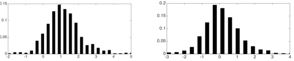
To determine the extent to which college educated workers (l0) compared to workers
with high school degrees in the same gender-age group (l) use computers (k0) relatively
more than non-computer equipment (k) within occupations (w), the left panel of Figure2
plots the histogram of
logpt l0,k0,w
pt l0,k,w log
pt l,k0,w
pt l,k,w
23We observep
t(l,k,w) =0 in the data for roughly 27% of(l,k,w)observations in any given year. As
a robustness check, in AppendixE.2we drop age and consider 10 labor groups, reducing the share of zero allocations.
24The GermanQualification and Working Conditionssurvey, used in e.g.DiNardo and Pischke(1997), helps
mitigate the second and third concerns by providing data on worker usage of multiple types of equipment and, in 2006, the share of hours spent using computers. In AppendixCwe show using this more detailed German data similar patterns of comparative advantage—between computers and education groups and between computers and gender—as in the U.S. data described below. We do not conduct our accounting exercise for Germany because wage data is noisy in publicly available datasets, see e.g. Dustmann et al. (2009), and because the GermanQualification and Working Conditionssurvey contains many fewer observa-tions than the October Supplement (depending on the year, between roughly 10,700 and 21,150 observaobserva-tions after cleaning).
across all five years, thirty occupations, and six gender-age groups. Clearly, college edu-cated workers are relatively more likely to use computers within occupations compared to high school educated workers. A similar pattern holds comparing across other educa-tion groups.
Figure 2: Computer relative to non-computer usage for college degree relative to high school degree workers (female relative to male workers) in the left (right) panel
The right panel of Figure 2 plots a similar histogram, where l0 and l denote
fe-male and fe-male workers, respectively, across all five years, thirty occupations, and fifteen education-age groups. This figure shows that on average there is no clear difference in computer usage across genders within occupations (i.e. the histogram is roughly cen-tered around zero). Hence, in order to account for the fact that women use computers more than men at the aggregate level—see Table 1—women must have a comparative advantage in the occupations in which computers have a comparative advantage.
We can similarly study the extent to which labor groups differ in their allocations across occupations conditional on computer usage and the extent to which computers differ in their allocations across occupations conditional on labor groups. For instance, using similar histograms we can show that women are much more likely than men to work in administrative support relative to construction occupations, conditional on the type of equipment used; and that computers are much more likely to be used in adminis-trative support than in construction occupations, conditional on labor group. These com-parisons provide an example of a more general relationship: women tend to be employed in occupations in which all labor groups are relatively more likely to use computers.
3.2 Measuring shocks
Here we describe our baseline procedure to measure shocks to labor composition, ˆL(l)/ ˆL(l1), equipment productivity, ˆq(k)q/ ˆq(k1)q, occupation shifters, ˆa(w)/ ˆa(w1), and labor pro-ductivity, ˆT(l)/ ˆT(l1). We measure changes in labor composition directly from the MORG CPS. We measure changes in equipment productivity using data only on changes in de-tailed allocations over time, ˆp(l,k,w). We measure changes in occupation shifters using
data on detailed allocations and labor income shares across occupations over time as well as model parameters. Finally, we measure changes in labor productivity as a residual to match changes in relative wages. Details are provided in AppendixB.1and we provide variations of this baseline procedure in AppendicesB.2andB.3, each of which yields very similar results.
Consider first our measure of changes in equipment productivity. Equations (3) and (6) give
ˆ q(k)q ˆ
q(k1)q = ˆ
p(l,k,w)
ˆ
p(l,k1,w) (10)
for any (l,w) pair. Hence, if computer productivity rises relative to other equipment
between t0 and t1, then the share of l hours spent working with computers relative to other equipment in occupation w will increase. It is important to condition on (l,w)
pairs when identifying changes in equipment productivity because unconditional growth over time in computer usage, shown in Table 1, may also reflect growth in the supply of labor groups who have a comparative advantage using computers and/or changes in occupation shifters that are biased towards occupations in which computers have a comparative advantage. To construct changes in equipment productivity, we average the right-hand side of equation (10) over(l,w)pairs, as described in AppendixB.1.
Second, consider our measure of changes in occupation shifters. Equation (9) gives ˆ
a(w)
ˆ
a(w1) = ˆ
z(w)
ˆ
z(w1)
✓ qˆ
(w)
ˆ q(w1)
◆(1 a)(r 1)
. (11)
In order to construct occupation shifters, we construct the right-hand side of equation (11) as follows. We use equations (3) and (6) to obtain measures of changes in transformed occupation prices to the powerq(henceforth, in an abuse of terminology we will refer to
these as occupation prices) betweent0andt1, ˆ
q(w)q
ˆ
q(w1)q = ˆ
p(l,k,w)
ˆ
p(l,k,w1) (12)
for any (l,k) pair, which we average over (l,k) pairs as described in Appendix B.1.25
Hence, if the price ofw rises relative tow1 betweent0and t1, then the share of lhours spent working withkin occupationwrelative to in occupationw1will increase. As above, it is important to condition on (l,k) when identifying changes in occupation prices.
Given values of a, r, and q, we recover (qˆ(w)/ ˆq(w1))(1 a)(r 1). Next, given values of
25In calculating changes in relative wages in response to a subset of shocks, we solve for counterfactual
ˆ
q(k)q/ ˆq(k1)q and ˆq(w)q/ ˆq(w1)q, we construct ˆz(w)/ ˆz(w1) using the right-hand side of equation (9). Note that ifr = 1, changes in occupation shifters depend only on changes
in the share of labor payments across occupations.
Finally, we measure changes in labor productivity as a residual to match changes in relative wages, expressing equation (7) as
ˆ w(l)
ˆ
w(l1) = ˆ T(l)
ˆ T(l1)
✓ sˆ
(l)
ˆ s(l1)
◆1/q
. (13)
ˆ
s(l) is a labor-group-specific weighted average of changes in transformed equipment
and occupation prices, both raised to the powerq,
ˆ
s(l) =
Â
k,wˆ q(w)q
ˆ q(w1)q
ˆ q(k)q ˆ q(k1)q
pt0(l,k,w), (14)
which we can construct using observed allocations and measured changes in equipment productivity and occupation prices. Clearly, we require a value ofq to measure changes
in labor productivity. Note that changes in relative wages only directly affect our mea-sures of changes in labor productivities. Wage changes have no effect on our meamea-sures of changes in labor composition or equipment productivity and they only affect our mea-sures of occupation shifters indirectly through their impact on ˆz(w)/ ˆz(w1).26
3.3 Parameter estimates
Here we assign values to the parameters a, q, and r. The parameter a determines
pay-ments to all equipment (computers and non-computer equipment) relative to the sum of payments to equipment and labor. We seta =0.24, consistent with estimates inBurstein
et al.(2013).
3.3.1 Estimatingq
Equation (13) can be expressed as
26Because our measure of changes in equipment productivity are independent of worker wages, the
DiNardo and Pischke(1997) critique ofKrueger(1993) does not apply to our approach. More generally, DiNardo and Pischke(1997) argue that measuring the impact of computers on wages requires taking into account two issues: “(1) computers are only productive in conjunction with a specific set of skills (e.g., programming); and (2) computers are of value only in certain jobs (e.g., for empirical economists but not for ballet dancers).” Our framework is designed precisely to address these issues. By allowing for comparative advantage between computers and labor groups we address issue (1) and by allowing for comparative advantage between computers and occupations we address issue (2).
log ˆw(l) =Vq(t) +bqlog ˆs(l) +iq(l). (15) We directly observe log ˆw(l), Vq(t) ⌘ log ˆq(w1)qˆ(k1) is a time effect that is common across l, bq ⌘ 1/q is the coefficient of interest, we construct log ˆs(l) using our pre-vious estimates, and iq(l) ⌘ log ˆT(l) captures unobserved changes in labor group l productivity (measuring changes in labor productivity requires a value ofq according to
equation (13)).
Regressing log ˆw(l) on log ˆs(l) would generate biased estimates ofbq, and therefore q, because changes in equilibrium occupation prices, ˆq(w), depend on changes in
un-observed labor productivity, iq(l). Specifically, we expect the error term iq(l) and the
covariate log ˆs(l)to be negatively correlated: the higher the growth in the productivity of
a particular labor group, the lower the growth in the price of those occupations that use that type of labor more intensively. Therefore, we expect the OLS estimate of bq to be bi-ased downwards and the estimate ofqto be biased upwards. To address the endogeneity
of the covariate log ˆs(l), we construct the following instrument for log ˆs(l),
cq(l) ⌘log
Â
kˆ q(k)q ˆ
q(k1)q
Â
w p1984(l,k,w),which is a labor-group-specific average of the observed changes in equipment productiv-ity ˆq(k)q/ ˆq(k
1)q. An increase in the relative productivity ofkbetweent0andt1raises the wage of grouplrelatively more if a larger share oflworkers use equipmentkin period
t0. While in our model we have not imposed assumptions on the stochastic structure of the shocks, a sufficient condition for our estimator to be consistent is that, in any two pe-riodst0and t1, the change in unobserved labor productivity, log ˆT(l), and the weighted changes in equipment productivity are uncorrelated across labor groups. In constructing the instrument for log ˆs(l) between any two periods t0 and t1, we could have used the observed labor allocations at period t0. However, in order to minimize the correlation between a possibly serially correlatediq(l)and the instrument, we construct our
instru-ment for log ˆs(l)between any two sample periodst0andt1using allocations in the initial sample year, 1984.
We estimateq(andrbelow) using four time periods: 1984-1989, 1989-1993, 1993-1997,
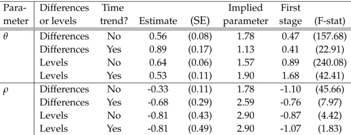
and 1997-2003. The resulting IV estimate isbq =0.56, with a robust standard error of 0.08. The F-stat in the first stage is 157 and the coefficient on the instrument has the expected positive sign; see Table2for details. This estimate impliesq =1.78.27
27If we had estimatedb
qusing an OLS estimator then we would have obtained an estimate ofbq =0.38,
which would implyq=2.61. The fact that the OLS estimate ofbqis lower than its IV estimate is consistent
Para- Differences Time Implied First
meter or levels trend? Estimate (SE) parameter stage (F-stat)
q Differences No 0.56 (0.08) 1.78 0.47 (157.68)
Differences Yes 0.89 (0.17) 1.13 0.41 (22.91) Levels No 0.64 (0.06) 1.57 0.89 (240.08) Levels Yes 0.53 (0.11) 1.90 1.68 (42.41)
r Differences No -0.33 (0.11) 1.78 -1.10 (45.66)
Differences Yes -0.68 (0.29) 2.59 -0.76 (7.97) Levels No -0.81 (0.43) 2.90 -0.87 (4.42) Levels Yes -0.81 (0.49) 2.90 -1.07 (1.83) Table 2: Parameter estimates
Notes: Estimate refers tobq in the first four rows andbrin the last four rows. We report
Huber-White standard errors (SE). First stage reports the coefficient on the instrument in the first stage regression and the final column reports the Kleibergen-Paap Wald rk F statistic (F-stat).
Alternative estimations of q. Here we show that our baseline estimate of q is robust to
a number of alternative estimation approaches. We use these alternative estimates in our sensitivity analyses in Section5.1.
First, Acemoglu (2002b) raises a concern that the presence of common trends in un-observed labor-group-specific productivity, explanatory variables, and instruments may bias the estimates of wage elasticities. Here we show that our estimate ofq is robust
ac-counting for labor-group-specific time trends in equation (15). Specifically, we express ˆ
T(l) as following al-specific time trend with deviations around this trend, log ˆT(l) =
bq(l)⇥(t1 t0) +iq1(l), which is the same assumption imposed inKatz and Murphy (1992) and in the estimation of the canonical model more generally. We then estimate
log ˆw(l) = Vq(t) +bq(l)⇥(t1 t0) +bqlog ˆs(l) +iq(l)
instead of equation (15) using the same instrumental variable for log ˆs(l)as in our
base-line approach. Here we identify our parameter of interest, bq, using variation in
devia-tions from trend in wage changes and predicted changes in labor-group-specific averages of the product of equipment productivity and occupation prices, log ˆs(l), instrumented
by the corresponding variation in deviations from trend in the variable cq(l). A suf-ficient condition for our estimator to be consistent is that, conditional on a linear time trend, in any two periodst0andt1, the change in unobserved labor productivity and the weighted changes in equipment productivity are uncorrelated across labor groups. This approach impliesq =1.13, as reported in Table2.
Second, whereas it is (slightly) simpler to take our framework to the data using time differences, in AppendixB.4we show how to estimatequsing a version of equation (15)
in levels and expanding the right-hand side variables with l-specific fixed effects. This
approach implies q = 1.48, as reported in Table 2. Third, we can combine both of the
previous approaches, including a labor-group-specific time trend and using levels with
l-specific fixed effects. This approach impliesq =2.04, as reported in Table2.
Fourth, according to our theory, labor composition only affects wages indirectly through occupation prices. We test this prediction by including changes in labor supply as an ad-ditional explanatory variable in equation (15). This yields an estimate of bq =0.54 that is
not statistically different from our baseline; this estimate impliesq = 1.84. Moreover, we
cannot reject at the 10% significance level the null hypothesis that the effect of changes in labor supply on changes in wages, conditional on the composite term log ˆs(l), is equal to
zero.
Finally, in AppendixDwe take an alternative approach—based onLagakos and Waugh (2013) andHsieh et al.(2013)—in which we use the empirical distribution of wages within eachlto estimatequsing maximum likelihood. This approach yieldsq =2.62.28
3.3.2 Estimatingr
Equation (9) can be expressed as
log ˆz(w) = Vr(t) +brlog qˆ(w) q ˆ q(w1)q
+ir(w). (16)
We directly observe log ˆz(w)in the MORG CPS,Vr(t) ⌘log ˆE+ (1 a) (1 r)log ˆq(w1) is a time effect that is common acrossw, br ⌘ (1 a) (1 r)/q is the coefficient of in-terest, we measure log ˆq(w)q/ ˆq(w1)q following the procedure indicated in Section3.2, and ir(w) ⌘ log ˆa(w) captures unobserved changes in occupation shifters (measuring changes in occupation shifters requires a value ofraccording to equation (11)).
According to our model, regressing log ˆz(w)on log ˆq(w)q/ ˆq(w1)q would generate bi-ased estimates of br, and therefore r because changes in equilibrium occupation prices,
ˆ
q(w), depend on changes in unobserved occupation shifters, ir(w). Specifically, we ex-pect the error termir(w)and the covariate log ˆq(w)q/ ˆq(w1)q to be positively correlated: the higher the growth in the occupation shifter of a particular occupation, the higher the growth in the occupation prices. Therefore, we expect the OLS estimate ofbrto be biased upwards. To address the endogeneity of the covariate log ˆq(w)q/ ˆq(w
1)q , we construct
the following Bartik-style instrument for log ˆq(w)q/ ˆq(w 1)q ,
cr(w) ⌘log
Â
kˆ q(k)q
ˆ
q(k1)q
Â
lL1984(l)p1984(l,k,w) Âl0,k0L1984(l0)p1984(l0,k0,w)
,
which is an occupation-specific average of the observed changes in equipment produc-tivity, ˆq(k)q/ ˆq(k1)q. An increase in the relative productivity of k raises occupation w’s output—and, therefore, reduces its price—relatively more if a larger share of workers employed in occupation w use equipment k in period t0. While in our model we have not imposed assumptions on the stochastic structure of the shocks, a sufficient condi-tion for our estimator to be consistent is that the change in the (unobserved) occupacondi-tion shifter and the weighted changes in equipment productivity are uncorrelated across oc-cupations.29 In order to minimize the correlation between a possibly serially correlated
ir(w) and the instrument, we construct our instrument using allocations in 1984, where L1984(l)p1984(l,k,w)is the number oflworkers using equipmentkemployed in occu-pationwin 1984 whereas the denominator is total employment inwin 1984.
The resulting IV estimate isbr = 0.33, with a robust standard error of 0.11. Together with our baseline values of a andq, this impliesr =1.78, as reported in Table 2. The
F-stat in the first stage is 45 and the coefficient on the instrument has the expected negative sign.30
Alternative estimations of r. Here we show that our baseline estimate ofr is robust to
a number of alternative approaches to the estimation ofbr. We use these alternative esti-mates in our sensitivity analyses in Section5.1. In each case we use our baseline estimates ofa andqto constructrfrom our estimate ofbr.
We obtain similar estimates ofrif we incorporate an occupation-specific time trend in
equation (16). In this case, we implicitly decompose ˆa(w) into an w-specific time trend
and deviations around this trend, log ˆa(w) = br(w)⇥(t1 t0) +ir1(w). We then esti-mate
log ˆz(w) =Vr(t) +br(w) (t1 t0) +brlog qˆ(w) q ˆ q(w1)q
+ir1(w),
29Theoretically, if the U.S. specializes in traded sectors that employ a large share of computer-intensive
occupations, then a rise in trade between 1984 and 2003 might generate a demand shift towards computer-intensive occupations within traded sectors, inducing a potential correlation between occupation shifters and weighted changes in equipment productivity. In practice, however, we find that computer-intensive occupations do not grow faster relative to computer-intensive occupations in manufacturing than non-manufacturing, suggesting that this theoretical concern is not a problem in practice.
30If we had estimated b
r using an OLS estimator then we would have obtained an estimate of br =
0.23, which would implyr = 0.46. The fact that the OLS estimate ofbr is higher than its IV estimate is
consistent with the prediction of our model that the error termir(w)should be negatively correlated with
instead of equation (16) using the same instrument as in our baseline approach. A suf-ficient condition for this estimator to be consistent is that, for any interval t0 and t1, the deviations from linear time trends in the changes in the unobserved occupation shifters and the weighted changes of equipment productivity are uncorrelated across occupa-tions. This approach impliesr=2.59, as reported in Table2.
In AppendixB.4 we show how to estimaterusing levels with w-specific fixed effects
rather than time differences. This approach impliesr=2.9 whether or not we incorporate
occupation-specific time trends, although in this case the instrument is weak when we include occupation-specific time trends, as reported in Table2.
4 Results
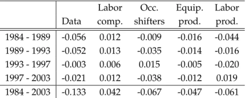
In this section we summarize our baseline results, quantifying the implications for rela-tive wages of changes in labor composition, occupation shifters, equipment productivity, and labor productivity. We construct various measures of changes in between-group in-equality that aggregate wage changes across our thirty labor groups (e.g., the skill pre-mium). As is standard, when doing so, both in the model and in the data, we construct composition-adjustedwage changes; that is, for each aggregated measure we average wage changes across the corresponding labor groups using constant weights over time, as de-scribed in detail in AppendixA. For each measure of inequality we report its cumulative log change between 1984 and 2003, calculated as the sum of the log change over all sub-periods in our data.31 We also report the log change over each sub-period in our data.
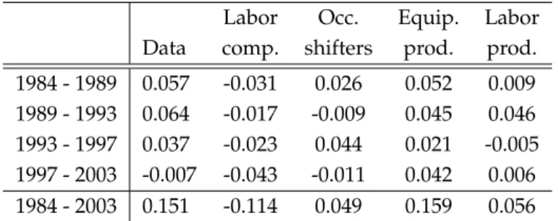
Skill premium. We begin by decomposing changes in the skill premium over the full sample period and over each sub-period, displayed in Table 3. The first column re-ports the change in the data, which is also the change predicted by the model when all changes—in labor composition, occupation shifters, equipment productivity, and labor productivity—are simultaneously considered. Between 1984 and 2003 the skill premium increased by 15.1 log points, with the largest increases occurring between 1984 and 1993. The subsequent four columns summarize the counterfactual change in the skill premium predicted by the model if only one component is changed (i.e. holding the other compo-nents at theirt0level).
Changes in labor composition decrease the skill premium over each sub-period in re-sponse to the large increase in the share of hours of more educated workers. The increase in hours worked by those with college degrees relative to those without of 47.4 log points
31For cumulative changes in log relative wages we obtain very similar results if we sett
0 = 1984 and