SOCIAL NETWORK
ABHIJIT BANERJEE†, ARUN G. CHANDRASEKHAR‡, ESTHER DUFLO§, AND MATTHEW O. JACKSON?
Abstract. Can we identify the members of a community who are best-placed to diffuse information simply by asking a random sample of in-dividuals? We show that boundedly-rational individuals can, simply by tracking sources of gossip, identify those who are most central in a network according to “diffusion centrality,” which nests other standard centrality measures. Testing this prediction with data from 35 Indian villages, we find that respondents accurately nominate those who are diffusion central (not just those with many friends). Moreover, these nominees are more central in the network than traditional village leaders and geographically central individuals.
JEL Classification Codes: D85, D13, L14, O12, Z13
Keywords: Centrality, Gossip, Networks, Diffusion, Influence, Social Learning
Date: This Version: August 2014.
Ben Golub, Michael Dickstein and participants at various seminars/conferences provided helpful comments. Financial support from the NSF under grants 1156182 and SES-1155302, from the AFOSR and DARPA under grant FA9550-12-1-0411, and from ARO MURI under award No. W911NF-12-1-0509 is gratefully acknowledged. We thank Fran-cisco Mu˜noz for excellent research assistance. We are grateful to CMF at IFMR, Tanay Balantrapu, Gowri Nagraj, and Manaswini Rao.
†Department of Economics, MIT.
‡Department of Economics, Stanford University. §Department of Economics, MIT.
?Department of Economics, Stanford University; Santa Fe Institute; and CIFAR.
1. Introduction
“The secret of my influence has always been that it remained secret.” – Salvador Dal´ı
Knowing who is influential, or central, in a community, can be important for the community’s members as well as for businesses and policymakers. In particular, the extent to which a piece of information diffuses among a popula-tion often depends on how central the initially informed are within the network (seeKatz and Lazarsfeld(1955);Rogers(1995);Kempe, Kleinberg, and Tardos
(2003, 2005); Borgatti (2005); Ballester, Calv´o-Armengol, and Zenou (2006);
Banerjee, Chandrasekhar, Duflo, and Jackson (2013)). Policymakers and or-ganizations can thus benefit from targeting the right individuals in efforts to effectively spread valuable information.
However, learning who is central in a social network has the potential to be difficult. For policymakers, collecting detailed network data is costly. Even for members of the community, knowing the structure of the network beyond their immediate friends is far from automatic. Do people know how central other people, outside of their immediate circle, are? In this paper, we answer this question theoretically and empirically.
First, we develop a simple model, building upon our previous work ( Baner-jee, Chandrasekhar, Duflo, and Jackson, 2013), to show that individuals in a network should be able to identify central individuals within their community without knowing anything about the structure of the network. Our model is about a process we call gossip, where nodes generate pieces of information that are then stochastically passed from neighbor to neighbor. We assume that individuals who hear the gossip are able to keep count of the number of times each person in the network get mentioned.1
We show that for any lis-tener in the network, the relative ranking under this count converges over time to the correct ranking of every node’s ability to send information to the rest
1We use the term “gossip” to refer to the spreading of information about particular people. Our diffusion process is focused on basic information that is not subject to the biases or ma-nipulations that might accompany some “rumors” (e.g., seeBloch, Demange, and Kranton
of the network. The specific measure of a node’s ability to send information that we use is given by the “diffusion centrality,” introduced in Banerjee et al.
(2013) which answers the question of how widely information from a given node diffuses in a given number of time periods and for a given random per period transmission probability. We relate diffusion centrality to other stan-dard measures of centrality in the literature, proving that it nests three of the most prominent measures: degree centrality at one extreme (if there is just one time period of communication), and eigenvector centrality and Katz-Bonacich centrality at the other extreme (if there are unlimited periods of communica-tion). For intermediate numbers of periods diffusion centrality takes on a wide range of other values.
In other words, by listening and keeping count of how often they hear about someone, individuals learn the correct ranking of community members from the point of view of how effectively they can serve as a source of information to the rest of the community.
Second, we use a unique dataset to assess whether this holds empirically. We asked every adult in each of 35 villages to name the person in their village best suited to initiate the spread of information. We combine their answers (which we call their “nominations”) with detailed network data that include maps of a variety of interactions in each of the 35 villages. We show that individuals nominate highly diffusion/eigenvector central people (on average at the 71st percentile of centrality). We also show that the nominations are not simply based on the nominee’s leadership status or geographic position in the village, but are significantly correlated with diffusion centrality even after conditioning on these characteristics, and are better predictors of centrality than these characteristics. This suggests that people understand our questions and are doing more than simply naming traditional leaders or geographically central individuals. Furthermore, there is suggestive evidence that they nominate people who are indeed diffusion central, not only people with many friends.
In sum, our model shows how individuals can learn who are the most central people in their network, and our empirical work suggests that individuals have learned this (although, of course, the data could be consistent with other models of how people choose individuals to nominate). To our knowledge, this
is the first paper to demonstrate that members of communities are able, easily and accurately, to identify highly central people in their community. It is also the first to describe a simple process by which people can learn things about part of their broader network that may intuitively seem outside their ambit.2
This is a result of practical importance, since asking people who is the best person to spread information is a much cheaper way to collect this information than collecting data on the entire network.
2. A Model of Network Communication
We consider the following model.
2.1. A Network of Individuals. A society of n individuals are connected via a possibly directed3 and weighted network, which has an adjacency matrix
g ∈ {0,1}n×n. Unless otherwise stated, we take the network g to be fixed
and let v(1) be its first (right-hand) eigenvector, corresponding to the largest
eigenvalue λ1.4 The first eigenvector is nonnegative and real-valued by the
Perron-Frobenius Theorem.
Throughout, we assume that the network is (strongly) connected in that there exists a (directed) path from every node to every other node, so that information originating at any node could potentially make its way eventually to any other node.5
2.2. Diffusion Centrality. Banerjee et al. (2013) defined a notion of cen-trality calleddiffusion centrality, based on random information flow through a network according to the following process, which is a variation of a standard diffusion process that underlies many contagion models.6
2There are some papers (e.g., Milgram(1967) and Dodds et al.(2003)) that have checked people’s abilities to use knowledge of their friends’ connections to efficiently route messages to reach distant people, but those rely on local knowledge.
3When defininggin the directed case, theij-th entry should indicate thatican tell some-thing toj. In some networks, this may not be reciprocal.
4v(1) is such thatgv(1)=λ
1v(1) whereλ1 is the largest eigenvalue ofgin magnitude. 5More generally, everything we say applies to the components of the network.
6SeeJackson and Yariv(2011) for background and references. A continuous time version of
A piece of information is initiated at node i and then broadcast outwards from that node. In each period, each informed node informs each of its neigh-bors of the piece of information and the identity of its original source with a probabilityp∈(0,1], independently across neighbors and history. The process operates for T periods, where T is a positive integer.
There are many reasons to allow T to be finite. For instance, a new piece of information may only be “news” for a limited time. Because of boredom, arrival of other news, the topic of conversation may change. By allowing for a variety of T’s, diffusion centrality admits important finite-horizon cases, as well as more extreme cases where agents discuss a topic indefinitely.7
Diffusion centrality measures how extensively the information spreads as a function of the initial node. In particular, let
H(g;p, T) :=
T X
t=1
(pg)t,
be the “hearing matrix.” The ij-th entry of H, H(g;p, T)ij, is the expected
number of times, in the firstT periods, that j hears about a piece of informa-tion originating from i. Diffusion centrality is then defined by
DC(g;p, T) :=H(g;p, T)·1=
T X
t=1
(pg)t
! ·1.
So, DC(g;p, T)i is the expected total number of times that some piece of
information that originates fromiis heard by any of the members of the society during a T-period time interval.8 Banerjee et al. (2013) showed that diffusion
7Of course this is an approximation and, moreover, different topics may have differentT’s. The current model and definition already moves beyond the literature, but even richer models could also be studied.
8 We note two useful normalizations. One is to compare it to what would happen ifp= 1 and g were the complete network gc, which produces the maximum possible entry for each ij subject to any T. Thus, each entry of DC(g;p, T) could be divided through by the corresponding entry of DC(gc; 1, T). This produces a measure for which every entry lies between 0 and 1, where 1 corresponds to the maximum possible numbers of expected paths possible in T periods with full probability weight and full connectedness. Another normalization is to compare a given node to the total level for all nodes; that is, to divide all entries ofDC(g;p, T) byP
iDCi(g;p, T). This normalization tracks how relatively diffusive one node is compared to the average diffusiveness in its society.
centrality was a statistically significant predictor of the spread of information – in that case, about a microfinance program.
Note that this measure allows people to hear the information multiple times from the same person and count those times as distinct reports, so that it is possible for an entry ofDC to be more than n. There are several advantages to defining it in this manner. First, although it is possible via simulations to calculate a measure that tracks the expected number of informed nodes and avoids double-counting, this expression is much easier to calculate and for many parameter values the two measures are roughly proportional to each other. Second, this version of the measure relates nicely to other standard measures of centrality in the literature, while a measure that adjusts for mul-tiple hearing does not. Third, in a world in which mulmul-tiple hearings lead to a greater probability of information retention, this count might actually be a better measure of what people learn.9
2.3. Diffusion Centrality’s Relation to Other Centrality Measures. It is useful to situate diffusion centrality relative to other prominent measures of centrality in the literature.
Letd(g) denote degree centrality (sodi(g) =Pjgij). Eigenvector centrality
corresponds to v(1)(g): the first eigenvector of g. Also, let KB(g, p) denote
Katz-Bonacich centrality – defined for p <1/λ1 by:10
KB(p,g) := ∞
X
t=1
(pg)t
! ·1.
It is direct to see that (i) diffusion centrality is proportional to degree cen-trality at the extreme at which T = 1, and (ii) if p < 1/λ1, then diffusion
centrality coincides with Katz-Bonacich centrality if we set T = ∞. We now show that when p >1/λ1 diffusion centrality approaches eigenvector
central-ity as T approaches ∞, which then completes the picture of the relationship between diffusion centrality and extreme centrality measures.
9One could also further enrich the measure by allowing for the forgetting of information, but with three parameters the measure would start to become unwieldy.
10See (2.7) inJackson(2008) for additional discussion and background. This was a measure first discussed by Katz, and corresponds to Bonacich’s definition when both of Bonacich’s parameters are set top.
The difference between the extremes of Katz-Bonacich centrality and eigen-vector centrality depends on whether p is sufficiently small so that limited diffusion takes place even in the limit of large T, or whether p is sufficiently large so that the knowledge saturates the network and then it is only relative amounts of saturation that are being measured.11
Theorem 1.
(1) Diffusion centrality is proportional to degree when T = 1:
DC(g;p,1) =pd(g).
(2) If p ≥ 1/λ1, then as T → ∞ diffusion centrality approximates
eigen-vector centrality: lim
T→∞
1
PT
t=1(pλ1)
tDC(g;p, T) =v (1).
(3) For T = ∞ and p < 1/λ1, diffusion centrality is Katz-Bonacich
cen-trality:
DC(g;p,∞) =KB(g, p) ; p <1/λ1.
All proofs appear in the Appendix.
The result shows that as T is varied, diffusion centrality nests three of the most prominent and used centrality measures: degree centrality, eigenvector centrality, and Katz-Bonacich centrality. It thus provides a foundation for these measures and spans between them.12, 13 Between these extremes, dif-fusion centrality measures how difdif-fusion process operates for some limited
11Saturation occurs when the entries ofP∞ t=1(pg)
t
·1diverge (note that in a [strongly] connected network, if one entry diverges, then all entries diverge). Nonetheless, the limit vector is still proportional to a well defined limit vector: the first eigenvector.
12This formalizes a result we mention in (Banerjee, Chandrasekhar, Duflo, and Jackson,
2013). An independent formalization appears inBenzi and Klymko (2014).
13We also remark on the comparison to another measure: the influence vector that appears in the DeGroot learning model (see, e.g.,Golub and Jackson(2010)). That metric captures how influential a node is in a process of social learning. It corresponds to the (left-hand) unit eigenvector of a stochasticized matrix of interactions rather than a raw adjacency matrix. While it might be tempting to use that metric here as well, we note that it is the right conceptual object to use in a process ofrepeated averaging through which individuals update opinions based on averages of their neighbors’ opinions. It is thus conceptually different from the diffusion process that we study. One can define a variant of diffusion centrality that works for finite iterations of DeGroot updating.
number of periods. Importantly, as in Banerjee et al. (2013), the behavior in the intermediate ranges can be more relevant for certain diffusion phenomena.
3. Relating Diffusion Centrality to Network Gossip
We now investigate whether and how individuals living in g end up with knowledge of others’ positions in the network that correlates with diffusion centrality without knowing anything about the network structure.
3.1. A Gossip Process. Diffusion centrality considers diffusion from the sender’s perspective. Let us now consider the same stochastic information diffusion process but from areceiver’s perspective. Over time, each individual hears information that originates from different sources in the network, and in turn randomly pass that information on. The society discusses each of these pieces of information for T periods. The key point is that there are many such topics of conversation, originating from all of the different individuals in the society, with each topic being passed along for T periods.
For instance, Arun may tell Matt that he has a new car. Matt then may tell Abhijit that “Arun has a new car,” and then Abhijit may tell Esther that “Arun has a new car.” Arun may also have told Ben that he thinks house prices will go up and Ben could have told Esther that “Arun thinks that house prices will go up”. In this model Esther keeps track of the cumulative number of times that bits of information that originated from Arun reach her and compares it with the same number for information that originated from other people. What is crucial therefore is that the news involves the name of the node of origin – in this case “Arun” – and not what the information is about. The first piece of news originating from Arun could be about something he has done (“bought a car”) but the second could just be an opinion (“Arun thinks house prices will go up”). Esther keeps track of the fact that she has heard two different pieces of information originating from Arun.
Recall that
H(g;p, T) =
T X
t=1
is such that the ij-th entry, H(g;p, T)ij, is the expected number of times j
hears a piece of information originating from i.
We define the network gossip heard by node j to be the j-th column of H,
N G(g;p, T)j :=H(g;p, T)·j.
Thus, N Gj lists the expected number of times a node j will hear a given
piece of news as a function of the node of origin of the information. So, if
N G(g;p, T)ij is twice as high asN G(g;p, T)kj thenj is expected to hear news
twice as often that originated at nodei compared to node k, presuming equal rates of news originating at i and k.
Note the different perspectives of DC and N G: diffusion centrality tracks how well information spreads from a given node, while network gossip tracks relatively how often a given node hears information from (or about) each of the other nodes.
To end this sub-section two remarks are in order. First, one could allow passing probabilities to differ by information type and pairs of nodes.14 Indeed,
in Banerjee et al. (2013) we allowed different nodes to pass information with different probabilities, and in Banerjee et al. (2014) we allow the probability of communication to depend on the listener’s network position. Although one can enrich the model in many ways to capture specifics of information passing, this simple version captures basic dynamics and relates naturally to centrality measures. Second, we could allow nodes to differ in how frequently they generate new information which is then transmitted to its neighbors. Provided this transmission rate is positively related to nodes’ centralities, the results that we present below still hold (and, in fact, the speed of convergence would be increased).
3.2. Identifying Central Individuals. With this measure of gossip in hand, we show how individuals in a society can estimate who is central simply by
14We can generalize our setup replacingpwith a matrixP. Now define
H(g;P, T) := T X
t=1
(P◦g)t !
.
HerePcan have entriesPij which allow the transmission probabilities to vary by pair. Note thatPij can depend on characteristics of those involve and encode strategic behavior based on the economics being modeled.
counting how often they hear gossip about others. We first show that, on average, individuals’ rankings of others according to how much gossip they hear about the others, given by N Gj, are positively correlated with diffusion
centrality.
Theorem2. For any(g;p, T),Pjcov(DC(g;p, T), N G(g;p, T)j) = var(DC).
Thus, in any network with differences in diffusion centrality among individu-als, the average covariance between diffusion centrality and network gossip is positive.
It is important to emphasize that although both measures, N Gi and DCi,
are based on the same sort of information process, they are really two quite different objects. Diffusion centrality is a gauge of a node’s ability to send information, while the network gossip measure tracks the reception of infor-mation by different nodes. Indeed, the reason that Theorem 2 is only stated for the sum rather than any particular individualj’s network gossip measure is that for smallT it is possible that some nodes have not even heard about other nodes, and moreover they might be biased towards their local neighborhoods.15
Next, we show that if individuals exchange gossip over extended periods of time, every individual in the network is eventually able to perfectly rank others’ centralities.
Theorem3. If p≥1/λ1, then as T → ∞every individualj’s ranking of
oth-ers under N G(g;p, T)j will be according to the ranking of diffusion centrality,
DC(g;p, T), and hence according to eigenvector centrality, v(1).
The intuition is that individuals hear (exponentially) more often about those who are more diffusion/eigenvector central, as the number of rounds of com-munication tends to infinity. As such, in the limit, they assess the rankings
15One might conjecture that more central nodes would be better “listeners”: for instance, having more accurate rankings than less central listeners after a small number of periods. Although this might happen in some networks, and for many comparisons, it is not guar-anteed. None of the centrality measures considered here ensure that a given node, even the most central node, is positioned in a way to “listen” uniformly better than all other less central nodes. Typically, even a most central node might be farther than some less central node from some other important nodes. This can lead a less central node to hear some things before even the most central node, and thus to have a clearer ranking of at least some of the network before the most central node. Thus, for smallT, the P
is important in Theorem2.
according to diffusion/eigenvector centrality correctly. The result implies that with very little computational ability beyond remembering counts and adding to them, agents come to learn arbitrarily accurately complex measures of oth-ers’ centralities, even for people with whom they do not associate.
More sophisticated strategies in which individuals try to infer network topol-ogy, could accelerate learning. Nonetheless, this result holds even in a minimal environment wherein individuals do not know the structure of the network and do not tag anything but the topic of conversation (“Arun has a new car”).
The restriction top≥1/λ1 is important. For example, asptends to 0, then
individuals hear with vanishing frequency about others in the network, and network distance between people can matter in determining whom they think is the most important.
4. Data
To investigate the theory presented above, we examine new data, coupled with detailed network data gathered from villages in rural Karnataka (India). The network data consist of network information combined with “gossip” data for 35 villages.
To collect the network data (described in more details in (Banerjee, Chan-drasekhar, Duflo, and Jackson,2013), and publicly available athttp://economics. mit.edu/faculty/eduflo/social), we surveyed adults regarding with whom they interact.16 We have data concerning 12 types of interactions for a given
survey respondent: (1) whose houses he or she visits, (2) who visit his or her house, (3) his or her relatives in the village, (4) non-relatives who socialize with him or her, (5) who gives him or her medical advice, (6) from whom he or she borrows money, (7) to whom he or she lends money, (8) from whom he or she borrows material goods (e.g., kerosene, rice), (9) to whom he or she lends material goods, (10) from whom he or she gets advice, (11) to whom he or she gives advice, (12) with whom he or she goes to pray (e.g., at a temple, church or mosque). Using these data, we construct one network for each village, at
16We have network data from 89.14% of the 16,476 households based on interviews with 65% of all adult individuals aged 18-55.
the household level where a link exists between households if any member of any household is linked to any other member of any other household in at least one of the 12 ways.17 The resulting objects are undirected, unweighted
networks at the household level.
To collect the gossip data, we later asked the adults the following two addi-tional questions:
(Loan) If we want to spread information about a new loan product to everyone in your village, to whom do you suggest we speak?
(Event) If we want to spread information to everyone in the village about tickets to a music event, drama, or fair that we would like to organize in your village, to whom should we speak?
Table 1. Summary Statistics
mean sd
households per village 196 61.70
household degree 17.72 (9.81)
clustering in a household’s neighborhood 0.29 (0.16) avg distance between nodes in a village 2.37 (0.33) fraction in the giant component 0.98 (0.01)
is a “leader” 0.13 (0.34)
nominated someone for loan 0.48 (0.16) nominated someone for event 0.38 (0.16)
was nominated for loan 0.05 (0.03)
was nominated for event 0.04 (0.02) number of nominations received for loan 0.45 (3.91) number of nominations received for event 0.34 (3.28)
Notes: for the variables nominated someone for loan (event) and was nom-inated for loan (event) we present the cross-village standard deviation.
Table 1 provides some summary statistics for our data. The networks are sparse: the average number of households in a village is 196 with a standard
17Individuals can communicate if they interact in any of the 12 ways, so this is the network of potential communications, and using this network avoids the selection bias associated with data-mining to find the most predictive subnetworks.
deviation of 61.7, while the average degree is 17.7 with a standard deviation of 9.8.
We see that only 5% of households were named in response to the Loan question (and 4% for the Event question) with a cross-village standard devia-tion of 3%. Thus there is a substantial concordance in who is named as a good initiator of diffusion within a village. In fact, conditional on being nominated, a household was nominated nine times on average.18 This is perhaps a first
indication that the answers may be meaningful.
The fact that less than half of the households were willing to name someone, is itself intriguing. Perhaps people are unwilling to offer an opinion when they are unsure of the answer19 or possibly were afraid of offending someone, given that they were asked to name just one person.
We label as “leaders” self-help group leaders, shopkeepers, teachers, etc.: 13% of households fall into this category. We use the term as it was defined by the microfinance organization Bharatha Swamukti Samsthe (BSS) as part of their strategy for identifying people to initiate diffusion for their product. BSS approached such social leaders because they were a priori likely to be important in the social learning process and thereby would contribute to more diffusion of microfinance. In our earlier work,Banerjee et al.(2013), we show that there is considerable variation in the centrality of these “leaders” in a network sense, and that this variation predicts the eventual take up of microfinance.
5. Empirical Analysis
Our theoretical results suggest that people can learn others’ diffusion or eigenvector centralities simply by tracking news they hear through the network. Thus, they should be able to name central individuals when asked whom to use as a “seed” for diffusion. If this is the case, such direct questions can easily be added to standard survey modules to identify central individuals without obtaining detailed network data.
18We work at the household level, in keeping withBanerjee et al.(2013) who used households as network nodes; a household receives a nomination if any of its members are nominated.
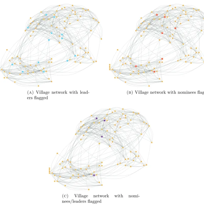
5.1. Descriptive Evidence. Figure1shows a village network where we high-light both the nominees and the village leaders used by BSS as seeds for micro-finance information, and thus the best guess of this organization of the most highly central people.20 We see in the figure that “leaders” include central
households but also some peripheral households. However, nominees appear to be more central and are rarely peripheral. Additionally, nodes that are both leaders and nominated are highly central.
Let us examine the relative network position of nominees in detail. Since the relevant number of periods to compute diffusion centrality is in principle application-dependent, we start with eigenvector centrality, which is a limit as
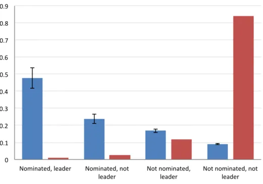
T → ∞of diffusion centrality for large enoughp(above the inverse of the first eigenvalue). We return to compare what happens with other pand T, below. Figure 2 builds on the theme presented in Figure 1. Examining the like-lihood that a nominated household is highly central, we find that 47% of households that are both nominated and have a leader are within the top 10% of the eigenvector centrality distribution. Furthermore, 23% of the households that are nominated but are not leaders are in the top decile of the centrality distribution.
This contrasts with households that are not nominated, irrespective of whether they have a leader. Only 16% of households that are not nominated but have a leader, and only 7% of households that are not nominated and have no leader, are in the top decile of the eigenvector centrality distribution.21 Another way to see this is that the average percentile in the distribution of eigenvector cen-trality for those nominated for the loan question is 0.71 (and 0.7 for event), while it is 0.62 for the traditional leaders.
Not only are nominated nodes more central in the network, but more central nodes also receive more nominations, as predicted by the theory. Figure 3
shows that households with higher levels of eigenvector centrality receive more
20This is not a geographic representation of nodes but, rather, a representation using a simple algorithm to visually represent the sub-community structure of the network. 21The difference between the 23% of households that are in the top decile given that they are nominated but not leaders and the 16% in the top decile given that they are not nominated but are leaders is significant with ap-value of 0.00 under a Welch test.
0 1 8 9 10 20 23 24 25 52 57 98 4 5 15 16 17 19 28 29 30 31 46 47 56 97 11 58 59 14 12 18 67 82 27 81 22 21 44 96 53 73 90 84 86 6 13 49 70 85 32 78 79 48 60 50 55 76 64 62 74 88 71 51 75 68 63 72 2 3 92 80 77 91 7 39 41 43 83 40 42 45 65 66 54 26 94 33 34 35 36 37 61 95 38 69 89 87 93
(a) Village network with lead-ers flagged 0 1 8 9 10 20 23 24 25 52 57 98 4 5 15 16 17 19 28 29 30 31 46 47 56 97 11 58 59 14 12 18 67 82 27 81 22 21 44 96 53 73 90 84 86 6 13 49 70 85 32 78 79 48 60 50 55 76 64 62 74 88 71 51 75 68 63 72 2 3 92 80 77 91 7 39 41 43 83 40 42 45 65 66 54 26 94 33 34 35 36 37 61 95 38 69 89 87 93
(b)Village network with nominees flagged
0 1 8 9 10 20 23 24 25 52 57 98 4 5 15 16 17 19 28 29 30 31 46 47 56 97 11 58 59 14 12 18 67 82 27 81 22 21 44 96 53 73 90 84 86 6 13 49 70 85 32 78 79 48 60 50 55 76 64 62 74 88 71 51 75 68 63 72 2 3 92 80 77 91 7 39 41 43 83 40 42 45 65 66 54 26 94 33 34 35 36 37 61 95 38 69 89 87 93
(c) Village network with nomi-nees/leaders flagged
Figure 1. A village network with nominees (red), leaders
(blue) and those who fulfill both categories (purple) flagged.
nominations on average than households of lower centrality, by a factor of about four when comparing the highest quintile to the lowest.
Figure 4 presents the distribution of nominations as a function of the net-work distance from a given household. If information did not travel well
0 0.1 0.2 0.3 0.4 0.5 0.6 0.7 0.8 0.9
Nominated, leader Nominated, not
leader Not nominated, leader Not nominated, not leader Probability of being in the top 10% of centrality PopulaCon share
Figure 2. The probability that a randomly chosen node with
a given classification (whether or not it is nominated under the event question and whether or not it has a village leader) is in the top decile of the eigenvector centrality distribution. 95% confidence intervals are displayed.
through the social network, we might imagine that individuals would only nominate households to whom they are directly connected. Panel A of Figure
4 shows that fewer than 20% of individuals nominate someone within their direct neighborhood. At the same time, over 27% of nominations come from a network distance of at least three or more. Taken together, this suggests that information about centrality does indeed travel through the network.
From Panel A of Figure 4, we also see that, while people do nominate individuals in households who are closer to them than the typical household in the village, respondents generally name people outside of their immediate neighborhoods and sometimes quite far. Moreover, it is important to note that highly central individuals are generally closer to people than the typical household, so, if they did nominate the most central people, this is what we should expect to find.
(a) Loan Question (b)Event Question
Figure 3. The average number of nominations per household
vs. the quintile of the households’ eigenvector centralities.
It is plausible that individuals may not have good information about who is central in parts of the network that are far from them. However, in Panel B of Figure 4 we see that the average eigenvector centrality percentile of those named at distance 1 is the same as at distance 2 or distance 3 or more. This suggests that individuals have reasonable and comparably accurate informa-tion about central individuals in the community who are immediate neighbors or at greater distance from them.
5.2. Regression Analysis. Motivated by this evidence, we present a more systematic analysis of the correlates of nominations, using a discrete choice framework for the decision to nominate someone.
Our theory suggests that if people choose whom to nominate by picking someone whom they hear about most frequently, then diffusion centrality should be a leading predictor of nominations. While the aforementioned re-sults are consistent with this prediction, there are several plausible alternative interpretations. For example, individuals may nominate the person with the most friends, and people with many friends tend to be more diffusion central than those with fewer friends (i.e., diffusion centrality with T = 1 and T >1
(a) Share of nominees in speci-fied neighborhood
(b)Average eigenvector centrality percentile of nominees in specified neighborhood
Figure 4. Distribution of centralities of nominees
can be positively correlated). Alternatively, it may be that people simply nom-inate “leaders” within their village, or people who are central geographically, and these also correlate with diffusion/eigenvector centrality. There are indeed a priori reasons to think that leadership status and geography may be good predictors of network centrality, since, as noted in Banerjee et al. (2013), the microfinance organization selected “leaders” precisely because they believed these people would be informationally central. Similarly, previous research has shown that geographic proximity increases the probability of link forma-tion (Fafchamps and Gubert, 2007; Ambrus et al., 2014; Chandrasekhar and Lewis, 2014) and therefore one might expect geographic data to be a useful predictor of centrality. In addition to leadership data we have detailed GPS coordinates for every household in each village. We include this in our analysis below.22
22To operationalize geographic centrality, we use two measures. The first uses the center of mass. We compute the center of mass and then compute the geographic distance for each agentifrom the center of mass. Centrality is the inverse of this distance, which we normalize by the standard deviation of this measure by village. The second uses the geographic data to construct an adjacency matrix. We denote theij entry of this matrix to be 1
d(i,j) where
d(·,·) is the geographic distance. Given this weighted graph, we compute the eigenvector centrality measure associated with this network. Results are robust to either definition.
Of course, the correlations below are not a “test” that the causal mechanism is indeed gossip, as in our model, but they do rule out that our diffusion centrality measure simply picks out degree centrality, geography or traditional leadership.
To operationalize our analysis using diffusion centrality, we need to first identify p and T. We use the average of the transmission probability pa-rameters estimated in Banerjee et al. (2013), which studies the diffusion of information about a loan, and finds p = 0.2. We set T = 3, since the aver-age distance between nodes in our network is 2.7 and thus 3 represents the distance to which information travels before it begins to echo backwards. In what follows, we use DC(0.2,3) when we refer to diffusion centrality.
We estimate a discrete choice model of the decision to nominate an individ-ual. Note that we have large choice sets as there are n−1 possible nominees and n nominators per village network. We model agent i as receiving utility
ui(j) for nominating individual j:
ui(j) =α+β0xj +γ0zj+µv +ij,v,
wherexjis a vector of network centralities forj(eigenvector centrality,DC(0.2,3),
and degree centrality),zj is a vector of demographic characteristics (e.g.,
lead-ership status, geographic position and caste controls), µv is a village fixed
effect, and iv,j is a Type-I extreme value distributed disturbance. For
conve-nience given the large choice sets, we estimate the conditional logit model by an equivalent Poisson regression, where the outcome is the expected number of times an alternative is selected (Palmgren, 1981; Baker, 1994; Lang, 1996;
Guimaraes et al., 2003).
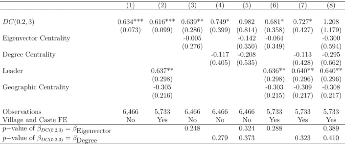
Table 2 presents our estimates of β and γ. First we show that DC(0.2,3) is a significant driver of an individual nominating another (column 1). A one standard deviation increase in eigenvector centrality is associated with a 0.634 log-point increase in the number of others nominating a household (statistically significant at the 1% level). In column 2 we see that this is robust to controlling for leadership status, geographic centrality of households, as well as village and caste fixed effects: a one standard deviation increase in diffusion centrality is associated with a 0.616 log-point increase in the number of others nominating
Table 2. Factors predicting nominations
(1) (2) (3) (4) (5) (6) (7) (8)
DC(0.2,3) 0.634*** 0.616*** 0.639** 0.749* 0.982 0.681* 0.727* 1.208
(0.073) (0.099) (0.286) (0.399) (0.814) (0.358) (0.427) (1.179)
Eigenvector Centrality -0.005 -0.142 -0.064 -0.300
(0.276) (0.350) (0.349) (0.594)
Degree Centrality -0.117 -0.208 -0.113 -0.295
(0.405) (0.535) (0.428) (0.662)
Leader 0.637** 0.636** 0.640** 0.640**
(0.298) (0.298) (0.296) (0.296)
Geographic Centrality -0.305 -0.303 -0.309 -0.308
(0.216) (0.215) (0.217) (0.217)
Observations 6,466 5,733 6,466 6,466 6,466 5,733 5,733 5,733
Village and Caste FE No Yes No No No Yes Yes Yes
p−value ofβDC(0.2,3)=βEigenvector 0.248 0.324 0.288 0.389
p−value ofβDC(0.2,3)=βDegree 0.279 0.373 0.323 0.410
Notes: The table reports estimate of a Poisson regression where the outcome variable is the expected number of nominations under the loan question. Degree centrality, eigenvector centrality andDC(0.2,3) are normalized by within-village standard deviation. Standard errors (clustered at the village level) are reported in parentheses. *** p <0.01, **p <0.05, *p <0.1.
the household (significant at the 1% level). Leadership status does affect the number of nominations as well, as we saw in the descriptive evidence, but the point estimate of the diffusion centrality coefficient hardly changes.
In columns 3-5 we add eigenvector and degree centrality as points of compar-ison. It seems that it is indeed diffusion centrality that best predicts nomina-tions. A one standard deviation inDC(0.2,3) corresponds to a 0.639 log-point increase in the number of nominations (statistically significant at the 5% level) as compared to -0.005 log-points when looking at eigenvector centrality (not statistically significant, column 3). Similarly, including both DC(0.2,3) and degree centrality leaves the coefficient onDC(0.2,3) mostly unchanged, a 0.749 log-point increase in the number of nominations associated with a one standard deviation increase in centrality, whereas there is no statistically significant as-sociation with degree centrality and the point estimate is considerably smaller (-0.117, column 4). However, parameter estimates are noisy and one cannot reject the hypothesis that the coefficients on DC(0.2,3) and eigenvector cen-trality as well as DC(0.2,3) and degree are statistically the same, despite the
difference in the point estimates. The p-values of a test of equality of coeffi-cients are 0.248 and 0.279 in columns 3 and 4, respectively (see the last row of the table). Further, we include all three centrality measures in column 5 and are unable to reject that any individual coefficient is statistically different from zero, although they are jointly significant with a p-value of 0.00). The point estimate of DC(0.2,3) remains similar to those in column 4, and both degree and eigenvector centrality have negative point estimates. However, due to the colinearity of the three centrality variables, standard errors are more than twice as large than in the previous columns. Columns 6-8 repeat the exer-cises of columns 3-5, now including leadership status and geographic centrality as extra control variables. Additionally, we add village and household caste fixed effects. As before we find that DC(0.2,3) enters significantly and with similar effect sizes, unless all three centralities are included, where the esti-mates become noisy. Moreover, in our pairwise comparisons neither degree nor eigenvector centrality coefficients are large and statistically significant drivers of the number of nominations.
Our results provide suggestive evidence that a key driver of the nomina-tion decision involves diffusion centrality with T >1 although, given the high degree of correlation of these metrics in our sample, we cannot statistically re-ject that all centrality variables matter equally. The point estimates, however, point towards the diffusion centrality as the most robust factor. Overall, it is clear that individuals are able to accurately name highly central individuals, well beyond using other status variables.
6. Concluding Remarks
Our model illustrates that it should be easy for even very myopic and non-Bayesian agents, simply by counting, to have an idea as to who is central in their community (according to fairly complex definitions). Motivated by this, we asked villagers to identify central individuals in their village. They do not simply name locally central individuals (the most central among those they know), but actually name ones that aregloballycentral within the village. This
suggests that individuals may use simple protocols to learn valuable things about the complex systems within which they are embedded.
Our findings have important policy implications, since such nomination data are easily collected and therefore can be used in a variety of contexts, either on its own, or combined with other easily collected data, to identify who would be a good seed for an information. For instance, if a household is both a nominee and a leader, it has a 47% likelihood of being in the top 10% of the centrality distribution.
It is also worth commenting that our work focuses on the network-based me-chanics of communication. In practice, considerations beyond simple network position may determine who the “best” person is to spread information, as other characteristics may affect the quality and impact of communication. An avenue for further research is to investigate whether villagers take such char-acteristics into account and thus may nominate individuals who are even more successful at diffusing information than the most central individual in the net-work. Beyond these, the work presented here opens a rich agenda for further research, as one can explore which other aspects of agents’ social environments can be learned in simple ways.
References
Alatas, V., A. Banerjee, A. G. Chandrasekhar, R. Hanna, and B. A. Olken (2014): “Network structure and the aggregation of
informa-tion: Theory and evidence from Indonesia,” NBER Working Paper. 19
Ambrus, A., M. Mobius, and A. Szeidl (2014): “Consumption
Risk-Sharing in Social Networks,”American Economic Review, 104, 149–82. 5.2 Baker, S. G.(1994): “The multinomial-Poisson transformation,”The
Statis-tician, 495–504. 5.2
Ballester, C., A. Calv´o-Armengol, and Y. Zenou (2006): “Who’s
who in networks, wanted: the key player,”Econometrica, 74, 1403–1417. 1 Banerjee, A., E. Breza, A. Chandrasekhar, E. Duflo, and M. Jackson (2014): “Come play with me: information diffusion about
Banerjee, A., A. Chandrasekhar, E. Duflo, and M. Jackson(2013):
“Diffusion of Microfinance,” Science, 341, DOI: 10.1126/science.1236498, July 26 2013. 1, 2.2, 12,2.3, 3.1, 4,4, 18, 5.2
Benzi, M. and C. Klymko(2014): “A matrix analysis of different centrality
measures,”arXiv:1312.6722v3. 12
Bloch, F., G. Demange, and R. Kranton (2014): “Rumors and Social
Networks,” Paris School of Economics, Working paper 2014 - 15. 1
Borgatti, S. P.(2005): “Centrality and network flow,”Social Networks, 27,
55 – 71. 1
Chandrasekhar, A. and R. Lewis (2014): “Econometrics of sampled
networks,” Stanford working paper. 5.2
Dodds, P. S., R. Muhamad, and D. J. Watts(2003): “An Experimental
Study of Search in Global Social Networks,” Science, 301, 827–829. 2 Fafchamps, M. and F. Gubert (2007): “The formation of risk sharing
networks,”Journal of Development Economics, 83, 326–350. 5.2
Golub, B. and M. Jackson (2010): “Naive Learning in Social Networks
and the Wisdom of Crowds,”American Economic Journal: Microeconomics, 2, 112–149. 13
Guimaraes, P., O. Figueirdo, and D. Woodward(2003): “A tractable
approach to the firm location decision problem,” Review of Economics and Statistics, 85, 201–204. 5.2
Jackson, M. (2008): Social and Economic Networks, Princeton: Princeton
University Press. 10
Jackson, M. and L. Yariv (2011): “Diffusion, strategic interaction, and
social structure,”Handbook of Social Economics, San Diego: North Holland, edited by Benhabib, J. and Bisin, A. and Jackson, M.O. 6
Katz, E. and P. Lazarsfeld(1955): Personal influence: The part played
by people in the flow of mass communication, Free Press, Glencoe, IL. 1
Kempe, D., J. Kleinberg, and E. Tardos (2003): “Maximizing the
Spread of Influence through a Social Network,” Proc. 9th Intl. Conf. on Knowledge Discovery and Data Mining, 137 – 146. 1
——— (2005): “Influential Nodes in a Diffusion Model for Social Networks,” In Proc. 32nd Intl. Colloq. on Automata, Languages and Programming, 1127
– 1138. 1
Lang, J. B. (1996): “On the comparison of multinomial and Poisson
log-linear models,” Journal of the Royal Statistical Society. Series B (Method-ological), 253–266. 5.2
Lawyer, G. (2014): “Understanding the spreading power of all nodes in a
network: a continuous-time perspective,” arXiv:1405.6707v2. 6 Milgram, S. (1967): “The small world problem,” Psychology Today. 2 Palmgren, J. (1981): “The Fisher information matrix for log linear models
arguing conditionally on observed explanatory variables,” Biometrika, 563– 566. 5.2
Appendix A. Proofs
We prove all of the statements for the case of weighted and directed net-works.
Letv(L,k) indicatek-th left-hand side eigenvector ofgand similarly letv(R,k)
indicate g’s k-th right-hand side eigenvector. In the case of undirected net-works, v(L,k) =v(R,k). In the case of directed networks, eigenvector v(1) in the main body corresponds to v(R,1).
The following lemma is used in proofs of the theorems.
Lemma 1. Consider a positive and diagonalizable g. Then g has a unique
largest eigenvalue. Moreover, letting ge =g/λ1,
[ge T]
ij →T v (R,1)
i v
(L,1)
j .
Proof of Lemma 1. The uniqueness of the largest eigenvalue follows from the Perron-Frobenius Theorem (given thatg is positive). By diagonalizability we can write g as
g=VΛV−1
where Λ is the matrix with eigenvalues on the diagonal (ordered from 1 tonin order of magnitude) andVis the matrix with columns equal to the right-hand eigenvectors, andV−1 is not onlyV’s inverse, but is also the matrix with rows
equal to the left-hand eigenvectors. By normalizing ge =g/λ1, it follows that e
g=VΛVe −1, whereΛ is the diagonal matrix such thate Λ = diage n
1,λe2, ...,λen
o
, and λek = λk
λ1. Since the largest eigenvalue of g is unique, it also follows that 0≤
λek
<1 for k >1.
It helps to write theik-th entry ofVasvi(R,k), and similarly, thekj-th entry of V−1 is written as v(L,k)
j . Therefore, it is straightforward to check that e
gTij =
n X
k=1
vi(R,k)v(L,k)j λeT k.
Separating terms,
e
gTij =vi(R,1)v(L,1)j +
n X
k=2
Thus, given that λfk T
→0 fork ≥2, it follows that
e
gTij →T→∞ v
(R,1)
i v
(L,1) j ,
as claimed.
Proof of Theorem 1. We show the second statement as the others follow directly.
First, note that in any neighborhood of any nonnegative matrix g, there exists a positive and diagonalizable matrixg0. Next, consider any nonnegative g. If the statement holds for any arbitrarily close positive and diagonalizable g0, then since PDC(T g;p,T)
t=1(pλ1)
t is a continuous function (in a neighborhood of a
non-negative and strongly connected g) as is the first eigenvector, the statement also holds at g. Thus, it is enough to prove the result for a positive and diagonalizable g, as in what follows.
In fact, we show the following strengthening of the statement for a positive and diagonalizable g.
• The ‘tail terms’ approach eigenvector centrality: (g/λ1)t·1→v(R,1) as t→ ∞.
• Ifp > λ−11, then
lim
T→∞
DC(g;p, T)
PT
t=1(pλ1)
t = limT→∞
DC(g;p, T)
pλ1−(pλ1)T+1
1−(pλ1)
=v(R,1).
• Ifp=λ−11, then
lim
T→∞ 1
TDC
g;λ−11, T=v(R,1).
By diagonalizability we write
g=VΛV−1,
and normalizing ge = g/λ1 it follows that ge =VΛVe
−1. Normalize the
sum to 1. Then, applying Lemma 1, it follows that ge
T ·1 is such that e
gT ·1 →v(R,1).
This completes the proof of the first statement. Next, we turn to the sumP∞
t=1ge
t·1and show the second statement for the
case where p= 1/λ1. It is sufficient to show
lim T→∞
DCg;λ−11, T
T −v
(R,1)
= 0.
First, note that as with our calculations above,
DCi
g;λ−11, T=X
j T X t=1 X k
v(R,k)i vj(L,k)λetk
Thus, DCi
g;λ−11, T
T −v
(R,1) i = P jPTt=1
Pn k=1v
(R,k)
i v
(L,k) j λetk
T −v
(R,1) i = = 1 T X j T X t=1 n X k=2
vi(R,k)vj(L,k)λet k ≤ 1 T T X t=1 n X k=2 1· n X j=1
vj(L,k)
| {z }
≤1 · λe t k ≤ n T T X t=1 λe t 2 = n T λe2
1− λe2
1− λe2
T →0.
Since the length of the vector (which is n) is unchanging in T, pointwise convergence implies convergence in norm, proving the result.
The final piece repeats the argument for p > 1/λ1, but now uses the
def-inition ge = (pg). Then we have Λ = diage n
e
λ1, ...,λen
o
with pλk = λek. We
show lim T→∞
DC(g;p, T)
PT
t=1(pλ1)t
−v(R,1)
By similar derivations as above, DCi
g;λ−11, T
PT t=1λet1
−v(R,1)i
= P jPTt=1
Pn k=1v
(R,k)
i v
(L,k) j λet
k PT
t=1λet1
−vi(R,1)
= = 1 PT t=1λet1
X j T X t=1 n X k=2
vi(R,k)vj(L,k)λet k
≤ PT1 t=1λet1
T X t=1 n X k=2 1· n X j=1
v(L,k)j
· λe t k ≤ n PT
t=1λet1 T X t=1 λe t 2 .
Note that this last expression converges to 0 since λe1 > 1, and λe1 > λe2.23
which completes the argument.
Proof of Theorem 2. Recall thatH=PTt=1(pg)tandDC=PTt=1(pg)t·1 and so
DCi =
X
j
Hij.
Additionally,
cov(DC, H·,j) =
X
i
DCi−
X
k
DCk
n
!
Hij −
X k Hkj n ! . Thus X j
cov(DC, H·,j) =
X
i
DCi−
X k DCk n ! X j
Hij −
X
k P
jHkj
n , implying X j
cov(DC, H·,j) =
X
i
DCi−
X
k
DCk
n
!
DCi−
X
k
DCk
n
!
= var(DC),
23Note that it is important thatp≥1/λ
1for this claim, since ifp <1/λ1, thenpλ1<1. In that case, observe that
PT t=1
˜λ2
t
PT t=1λ˜
t 1
= eλ2 e
λ1
· 1−λ˜1
1−λ˜2
by the properties of a geometric sum, which is of constant order. Thus, higher order terms (eλ2, etc.) persistently matter and are not dominated relative toPT
which completes the proof.
Proof of Theorem 3. Again, we prove the result for a positive diagonaliz-able g, noting that it then holds for any (nonnegative) g.
Again, letg be written as
g=VΛV−1.
Also, let ˜λk =pλk. It then follows that we can write
H=
T X
t=1
(pg)t =
T X t=1 n X k=1
vi(R,k)vj(L,k)λet k
!
.
By the ordering of the eigenvalues from largest to smallest in magnitude, H·,j =
T X
t=1
v(R,1)v(L,1)j ˜λt1+v(R,2)vj(L,2)λ˜t2+O
λ˜2
t = T X t=1
v(R,1)v(L,1)j ˜λt1+O
˜ λ2 t
= v(R,1)vj(L,1)
T X
t=1
˜
λt1+O
T X t=1 ˜ λ2 t! .
So, since the largest eigenvalue is unique, it follows that H·,j
PT t=1λ˜t1
=v(R,1)vj(L,1)+O
PT t=1 λ˜2
t PT
t=1λ˜t1
.
Note that the last expression converges to 0 since λe1 >1, and λe1 >eλ2. Thus,
H·,j PT
t=1˜λt1
→v(R,1)v(L,1)j
for eachj. This completes the proof since each column ofHis proportional to
v(R,1) in the limit, and thus has the correct ranking for large enough T.24 Note
that the ranking is up to ties, as the ranking of tied entries may vary arbitrarily along the sequence. That is, ifvi(R,1) =v`(R,1), then the ranking thatj has over
24The discussion in Footnote23clarifies whyp >1/λ
iand`could vary arbitrarily withT, but their rankings will be correct relative to any other entries with higher or lower eigenvector centralities.