When action is not least

When action is not least

C. G. Graya兲

Guelph-Waterloo Physics Institute and Department of Physics, University of Guelph, Guelph, Ontario N1G2W1, Canada

Edwin F. Taylorb兲

Department of Physics, Massachusetts Institute of Technology, Cambridge, Massachusetts 02139

共Received 17 February 2006; accepted 26 January 2007兲

We examine the nature of the stationary character of the Hamilton action S for a space-time

trajectory 共worldline兲 x共t兲 of a single particle moving in one dimension with a general

time-dependent potential energy functionU共x,t兲. We show that the action is a local minimum for sufficiently short worldlines for all potentials and for worldlines of any length in some potentials. For long enough worldlines in most time-independent potentialsU共x兲, the action is a saddle point, that is, a minimum with respect to some nearby alternative curves and a maximum with respect to others. The action is never a true maximum, that is, it is never greater along the actual worldline than along every nearby alternative curve. We illustrate these results for the harmonic oscillator, two different nonlinear oscillators, and a scattering system. We also briefly discuss two-dimensional examples, the Maupertuis action, and newer action principles. ©2007 American Association of Physics Teachers.

关DOI: 10.1119/1.2710480兴

I. INTRODUCTION

Several authors1–12have simplified and elaborated the ac-tion principle and recommended that it be introduced earlier into the physics curriculum. Their work allows us to see in outline how to empower students early in their studies with the fundamental yet simple extensions of Newton’s prin-ciples of motion made by Maupertuis, Euler, Lagrange, Ja-cobi, Hamilton, and others. The simplicity of the action prin-ciple derives from its use of a scalar energy and time. Its

transparency comes from the use of numerical11 and

analytical12 methods of varying a trial worldline to find a stationary value of the action, skirting not only the equations of motion but also the advanced formalism of Lagrange and others characteristic of upper level mechanics texts. The goal of this paper is to discuss the conditions for which the sta-tionary value of the action for an actual worldline is a mini-mum or a saddle point.

For single-particle motion in one dimension 共1D兲, the

Hamilton actionSis defined as the integral along an actual or trial space-time trajectory 共worldline兲 x共t兲 connecting two specified events PandR,

S=

冕

P R

L共x,x˙,t兲dt, 共1兲 whereLis the Lagrangian,xis the position,tis the time, and

P共xP,tP兲 and R共xR,tR兲 are fixed initial and final space-time

events. A dot, as in x˙, indicates the time derivative. The LagrangianL共x,x˙,t兲depends ontimplicitly throughx共t兲and may also depend ontexplicitly, for example, through a time-dependent potential. For simplicity we use Cartesian coordi-nates throughout, but the methods and conclusions apply for generalized coordinates.

The Hamilton action principle compares the numerical value of the actionS along the actual worldline to its value along every adjacent curve 共trial worldline兲anchored to the same initial and final events. These alternative curves are arbitrary as long as they are piecewise smooth, have the same end events, and are adjacent to 共near to兲 a worldline

that the particle will indeed follow. For example, the adjacent curves need not conserve the total energy. The Hamilton ac-tion principle says that with respect to all nearby curves the action along the actual worldline is stationary, that is, it has

zero variation to first order; formally we write ␦S= 0.

Whether or not this stationary value of the action is a local

minimum is determined by examining␦2_{S and higher order}

variations of the action with respect to the nearby curves, as we will discuss in this paper.

Misconceptions concerning the stationary nature of the ac-tion abound in the literature. Even Lagrange wrote that the

value of the action can be maximum,13a common error14of

which the authors of this paper have been guilty.12,15Other

authors use extremum or extremal,16 which incorrectly

in-cludes a maximum and formally fails to include a saddle point. 关Mathematicians often use the共correct兲 term critical

instead of stationary, but because the former term has other meanings in physics we use the latter.兴A similar error mars treatments of Fermat’s principle of optics, which is errone-ously said to allow the travel time of a light ray between two

points to be a maximum.17

The present paper has three primary purposes: First it de-scribes conditions under which the action is a minimum and different conditions under which it is a saddle point. These conditions involve second variations of the action. Some pio-neers of the second variation theory of the calculus of varia-tions are Legendre, Jacobi, Weierstrass, Kelvin and Tait,

Mayer, and Culverwell.18 Although inspired by the early

work of Culverwell,21 our derivation of these conditions is new, simpler, and more rigorous; it is also simpler than mod-ern treatments.24,25 Second, this paper explains the results with qualitative heuristic descriptions of how a particle re-sponds to space-varying forces derived from the potential in

which it moves.共Those who prefer immediate immersion in

the formalism can begin with Sec. IV.兲 Third, it clarifies

these results and illustrates the variety of their consequences by applying them to the harmonic oscillator, two nonlinear oscillators, and a scattering system. Criteria used to decide

the nature of the stationary value of the action are also useful for other purposes in classical and semiclassical mechanics,28 but are not discussed in this paper.

Appendix A adapts the results to the important Maupertuis

actionW. Appendix B gives examples of both Hamilton and

Maupertuis action for two-dimensional motion. Appendix C discusses open questions on the stationary nature of action for some newer action principles.

II. KINETIC FOCUS

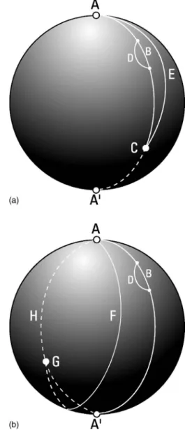
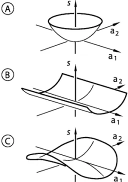
This section introduces the concept ofkinetic focusdue to Jacobi,22which plays a central role in determining the nature of the stationary action. We start with an analogous example taken verbatim from Whittaker,36 an analysis of the relative length along different paths. Whittaker employs the Mauper-tuis action principle 共discussed in our Appendix A兲, which requires fixed total energy along trial paths, not fixed travel time as with the Hamilton action principle. In force-free sys-tems the value of the Maupertuis action is proportional to the path length. The term kinetic focus is defined formally later in this section. Figures 1共a兲and 1共b兲illustrate this example. Whittaker wrote that “A simple example illustrative of the results obtained in this article is furnished by the motion of a particle confined to a smooth sphere under no forces. The trajectories are great-circles on the sphere and the关 Mauper-tuis兴action taken along any path共whether actual or trial兲is proportional to the length of the path. The kinetic focus of

any point A is the diametrically opposite point A

⬘

on the

sphere, because any two great circles through A intersect

again 共for the first time兲 atA

⬘

. The theorems of this article amount, therefore in this case to the statement that an arc of a great circle joining any two pointsAandBon the sphere is the shortest distance fromA toB when共and only when兲the pointA

⬘

diametrically opposite toA does not lie on the arc, that is, when the arc in question is less than half a great-circle.”

The elaboration of this analogy is discussed in the captions of Figs. 1共a兲and 1共b兲using equilibrium lengths of a rubber band on a slippery spherical surface.

For a contrasting example, we apply a similar analysis to free-particle motion in a flat plane. In this case the length of the straight path connecting two points is a minimum no matter how far apart the endpoints. A rubber band stretched between the endpoints on a slippery surface will always snap back when deflected in any manner and released. An alterna-tive straight path that deviates slightly in direction at the

initial point A continues to diverge and does not cross the

original path again. Therefore no kinetic focus of the initial pointAexists for the original path.

Note that on both the sphere and the flat plane there is no path of true maximum length between any two separated points. The length of any path can be increased by adding wiggles.

How do we find the kinetic focus? In Fig. 1共a兲 we place the terminal point C at different points along a great circle

path between A and A

⬘

. When C lies between A and A

⬘

,

every nearby alternative path such asAECis not a true path 共a path of minimum length兲, because it does not lie along a great circle. When terminal pointCreachesA

⬘

, there is sud-denly more than one alternative great circle path connecting

AandA

⬘

.共In this special case an infinite number of alterna-tive great circle paths connect A and A

⬘

.兲 Any alternative great circle path betweenAandA

⬘

can be moved sideways to

coalesce with the original path ABA

⬘

. The kinetic focus is defined by the existence of this coalescing alternative true path. As the final pointC moves away from the initial point

A, the kinetic focus A

⬘

is defined as the earliest terminal point at which two true paths can coalesce.

The term kinetic focus in mechanics derives from an analogy37to the focus in optics, that point A

⬘

at which rays Fig. 1.共a兲On a sphere the great circle lineABCstarting from the north pole atAis the shortest distance between two points as long as it does not reach the south pole atA⬘. On a slippery sphere a rubber band stretched between

AandCwill snap back if displaced either locally, as atD, or by pulling the entire line aside, as alongAEC. The pointA⬘is called theantipodeofAor in general thekinetic focusofA. We say that if a great circle path terminates before the kinetic focus of its initial point, the length of the great circle path is a minimum.共b兲If the great circleABA⬘Gpasses through antipodeA⬘of the initial pointA, then the resulting line has a minimum length only when compared with some alternative lines. For example on a slippery sphere a rubber band stretched along this path will still snap back from local distor-tion, as atD. However, if the entire rubber band is pulled to one side, as alongAFG, then it will not snap back, but rather slide over to the portion

AHGof a great circle down the backside of the sphere. With respect to paths likeAFG, the length of the great circle lineABA⬘Gis a maximum. With respect to all possible variations we say that the length of pathABA⬘Gis a saddle point. If a great circle path terminates beyond the kinetic focus of its initial point, the length of the great circle path is a saddle point.

emitted from an initial point Aconverge under some condi-tions, such as interception by a converging lens.

This paper deals mainly with the action principle for the

Hamilton action S, which determines worldlines in

space-time for fixed end-events 共that is, end-positions and travel time兲rather than the action principle for the Maupertuis ac-tionW共see Appendix A兲, which determines spatial orbits共as

well as space-time worldlines兲 for fixed end-positions and

total energy. The kinetic focus for the Hamilton action has a use similar to that for the examples of the Maupertuis action in Figs. 1共a兲 and 1共b兲. We will show that a worldline has a minimum actionSif it terminates before reaching the kinetic focus of its initial event. In contrast, a worldline that termi-nates beyond the kinetic focus of the initial event P has an action that is a saddle point.

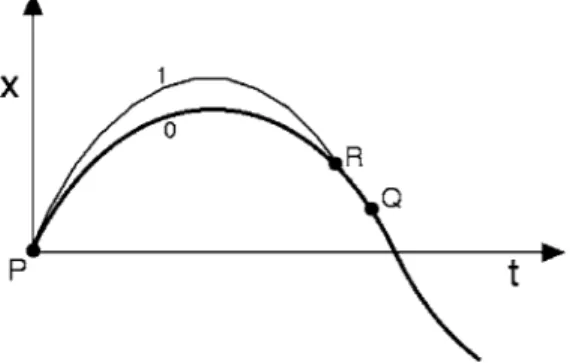
We use the labelPfor the initial event on the worldline 0 共see Fig. 2兲,Q for the kinetic focus of P on the worldline,

and R for a fixed but arbitrary event on the worldline that

terminates on worldline 0 and also terminates another true worldline共#1 in Fig. 2兲connectingPtoR. For the Hamilton actionS our definition of the kinetic focus of a worldline is the following. The kinetic focusQof an earlier eventPon a true worldline is the event closest toPat which a second true worldline, with slightly different velocity atP, intersects the first worldline, in the limit for which the two worldlines coa-lesce as their initial velocities atP are made equal.

The kinetic focus is central to the understanding of the stationary nature of the actionS, but its definition may seem obscure. To preview the consequences of this definition, we briefly discuss some examples that we will discuss later in the paper. Figure 3 shows the true worldlines of the harmonic

oscillator, whose potential energy has the form U共x兲

=

共

1₂

兲

kx2. The harmonic oscillator is the single 1D case of the definition of space-time kinetic focus with the following ex-ceptional characteristic: every worldline originating at P in Fig. 3 passes through the same recrossing point. The 2D spatial paths on the sphere in Figs. 1共a兲 and 1共b兲 show the

same characteristic: Every great circle path starting at A

passes through the antipode atA

⬘

. In both cases we can find the kinetic focus without taking the limit for which the ve-locities at the initial point are equal and the two worldlines coalesce, but we can take that limit. For the harmonic oscil-lator this limit occurs when the amplitudes are made equal. The harmonic oscillator will turn out to be the only excep-tion to many of the rules for the acexcep-tion.

A more typical case is the quartic oscillator 共see Fig. 4兲, which is described by U共x兲=Cx4_{. In this case alternative}

worldlines starting from the initial event P can cross

any-where along the original worldline共some crossing events are indicated by little squares in Fig. 4兲. When the alternative worldline coalesces with the original worldline, the crossing point has reached the kinetic focusQ.

Another typical case is the piecewise-linear oscillator shown in Fig. 5. This oscillator has the potential energy

U共x兲=C兩x兩. For the piecewise-linear oscillator, as for the quartic oscillator, alternative worldlines starting from P can cross at various events along the original worldline. Note that for the piecewise-linear oscillator an alternative world-line that crosses the original worldworld-line before its kinetic fo-cus lies below the original worldline instead of above it共as for the quartic oscillator兲. We can equally well use an alter-native worldline that crosses from below or one that crosses from above to define the coalescing worldline and kinetic focus.

Notice the gray line labeled causticin Figs. 4 and 5, and also in Fig. 6, which shows the worldlines for a repulsive Fig. 2. From the common initial eventPwe draw a true worldline 0 and a

second true worldline 1 that terminates at some event R on the original worldline 0. The event nearest to Pat which worldline 1 coalesces with worldline 0 is the kinetic focusQ.

Fig. 3. Several true harmonic oscillator worldlines with initial event P

=共0 , 0兲and initial velocityv0⬎0. Starting at the initial fixed eventPat the origin, all worldlines pass through the same eventQ. That is,Qis the kinetic focus for all worldlines of the family starting at the initial eventP=共0 , 0兲. Worldlines 1 and 0 differ infinitesimally; worldlines 2 and 0 differ by a finite amount. This oscillator is discussed in detail in Sec. VIII.

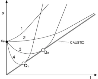
Fig. 4. Schematic space-time diagram of a family of true worldlines for the quartic oscillator关U共x兲=Cx4_{兴starting atP=共0 , 0兲withv}

0⬎0. The kinetic focus occurs at a fraction 0.646 of the half-periodT0/ 2, illustrated here for worldline 0. The kinetic foci of all worldlines of this family lie along the heavy gray line, the caustic. Squares indicate recrossing events of worldline 0 with the other two worldlines. This oscillator is discussed in detail in Sec. IX.

potential. The caustic is the line along which the kinetic foci lie for a particular family of worldlines共such as the family of worldlines that start from P with positive initial velocity in Figs. 4 and 5兲. A caustic is also an envelope to which all worldlines of a given family are tangent. The caustics in Figs. 5 and 6 are time caustics, envelopes for space-time trajectories共worldlines兲. Figure 7 shows a purely spatial caustic/envelope for a family of parabolic paths共orbits兲in a

linear gravitational potential. The word caustic is derived from optics37 共along with the word focus兲. When a cup of coffee is illuminated at an angle, a bright curved line with a cusp appears on the surface of the coffee共see Fig. 8兲. Each point on this spatial optical caustic or ray envelope is the focus of light rays reflected from a small portion of the cir-cular inner surface of the cup.

In Figs. 4–7 the caustic for a family of worldlines 共or

paths兲represents a limit for those worldlines 共or paths兲. No Fig. 5. Schematic space-time diagram of a family of true worldlines for a

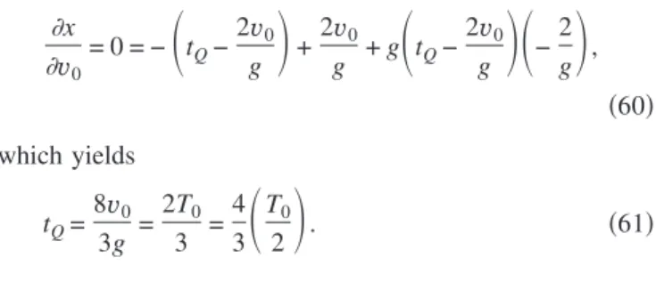
piecewise-linear oscillator关U共x兲=C兩x兩兴, with initial eventP=共0 , 0兲and ini-tial velocityv0⬎0. The kinetic focusQ0of worldline 0 occurs at

4 3 of its half-periodT0/ 2. Similarly, small circlesQ1andQ2are the kinetic foci of worldlines 1 and 2, respectively. The heavy gray curve is the caustic, the locus of all kinetic foci of different worldlines of this family共originating at the origin with positive initial velocity兲. Squares indicate events at which the other worldlines recross worldline 0. This oscillator is discussed in detail in Sec. IX.

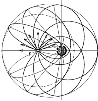
Fig. 6. Schematic space-time diagram for the repulsive inverse square po-tential关U共x兲=C/x2_{兴, with a family of worldlines starting atP共x}

P, 0兲with various initial velocities. Intersections are events where two worldlines cross. The heavy gray straight linexQ=共␥/xP兲tQ, where␥=共2C/m兲1/2, is the caustic, the locus of kinetic fociQ共open circles兲and envelope of the indi-rect worldlines. Worldline 2, with zero initial velocity, is asymptotic to the caustic, with kinetic focus Qat infinite space and time coordinates. The caustic divides space-time: each final event above the caustic can be reached by two worldlines of this family of worldlines, each final event on the caustic by one worldline of the family, and each final event below the caustic by no worldline of the family. This system is discussed in detail in Sec. X.

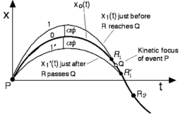
Fig. 7. For the Maupertuis action, the heavy line envelope共the “parabola of safety”兲is the locus of spatial kinetic foci共xQ,yQ兲, or spatial caustic, of the family of parabolic orbits of energy E originating from the origin

O共xP,yP兲=共0 , 0兲with various directions of the initial velocityv0. The po-tential isU共x,y兲=mgy. The horizontal and vertical axes arexandy, respec-tively, and the caustic/envelope equation isy=v₀2/ 2g−gx2_{/ 2v}

0

2_{, found by} Johann Bernoulli in 1692. The caustic divides space. Each final point

共xR,yR兲inside the caustic can be reached from initial point共xP,yP兲by two orbits of the family, each final point on the caustic by one orbit of the family, and each point outside the caustic by no orbit of the family.Yis the vertex

共highest reachable point y=v₀2_{/ 2g兲 of the caustic and X}

1, X2 denote the maximum range points共x= ±v₀2_{/g兲. This system is discussed in detail in} Appendix B.共Figure adapted from Ref. 43.兲

Fig. 8. The coffee-cup optical caustic. The caustic shape in panel 共b兲 共a nephroid兲was derived by Johann Bernoulli in 1692共Ref. 44兲.

worldline of that family exists for final events outside the caustic. At least one worldline can pass through any event inside the caustic. Exactly one worldline can pass through an event on the caustic, and this event is the worldline’s kinetic focus. This observation is consistent with the definition of the kinetic focus as an event at which two separate world-lines coalesce.

At the kinetic focus the worldline is tangent to the caustic. When two curves touch but do not cross and have equal slope at the point where they touch, the curves are said to

osculate or kiss, which leads to a summary preview of the results of this paper:

When a worldline terminates before it kisses the caustic, the action is minimum; when the worldline terminates after it kisses the caustic, the action is a saddle point.

One consequence is that when we use a computer to plot a

family of worldlines 共by whatever means兲, we can eyeball

the envelope/caustic and locate the kinetic focus of each worldline visually.

This summary covers every case but one, because when no kinetic focus exists, there is no caustic so a worldline of any length has the minimum action. The one case not cov-ered by this rule is the harmonic oscillator. For the harmonic oscillator and also for the sphere geodesics of Fig. 1, the caustic collapses to a single point at the kinetic focus. In this case there is no caustic curve; only one caustic point共a focal point兲 exists. A corresponding optical case is a concave re-flecting parabolic surface of revolution illuminated with in-coming light rays parallel to its axis; the optical caustic col-lapses into a single point at the focus 共focal point兲 of the parabolic mirror. When the optical caustic reduces to a point for a lens or mirror system, the resulting images have mini-mum distortion共minimum aberration兲.

For the quartic and the piecewise-linear oscillators 共and the harmonic oscillator兲 subsequent crossing points exist at which two worldlines can coalesce. We have defined the ki-netic focus as the first of these, the one nearest the initial

event P. The procedure for locating the subsequent kinetic

foci is identical to that for locating the first one and is dis-cussed briefly in the examples of Secs. VIII and IX. For 1D

potentials subsequent kinetic foci45 exist for the bound

worldlines but not for the scattering worldlines, for example, those in Fig. 6. We shall not be concerned with subsequent kinetic foci; when we refer to the kinetic focus we mean the first one, as we have defined it. We shall show in what fol-lows that for a few potentials 关for example, U共x兲=C and

U共x兲=Cx兴 kinetic foci do not exist, because true worldlines

beginning at a common initial eventP do not cross again.

The definition of kinetic focus in terms of coalescing worldlines provides a practical way to find the kinetic focus. In Fig. 2 note the slopes of nearby worldlines 1 and 0 at the initial event P. The initial slope of curve 1 is only slightly different from that of worldline 0; as that difference ap-proaches zero, the crossing event apap-proaches the kinetic

fo-cus Q. The slope of a worldline at any point measures the

velocity of the particle at that point. This coalescence of two worldliness as their initial velocities approach each other leads to a method for finding the kinetic focus: Launch an identical second particle from event P 共simultaneously with the original launch兲but with a slightly different initial

veloc-ity, that is, with a slightly different slope of the worldline. Worldline number 1 is also a true worldline. In the limiting case of a vanishing difference in the initial velocities at event

P 共vanishing angle between the initial slopes兲, the two

worldlines will cross again, and the two particles collide at the kinetic focus eventQ.

We can convert this practical共actually heuristic兲idea into an analytical method, often easily applied when we have an analytic expression for the worldline. Let the original world-line be described by the function x共t,v0兲, where v0 is the initial velocity. Then the second worldline is the same func-tion with incrementally increased initial velocity x共t,v₀ +⌬v0兲. We form the expansion in⌬v₀

x共t,v₀+⌬v0兲=x共t,v0兲+ ⳵x

⳵v₀⌬v0+O共⌬v0 2_兲

. 共2兲

At an intersection pointR we havex共tR,v0+⌬v0兲=x共tR,v0兲.

For intersection point RnearQwe therefore have

⳵x

⳵v0

⌬v0+O共⌬v02兲= 0, 共3兲

which implies that forR→Qwhen ⌬v0→0, we have

⳵x

⳵v0

= 0. 共4兲

Equation 共4兲 is an analytic condition for the incrementally different worldline that crosses the original worldline at the kinetic focus, and hence it locates the kinetic focus Q. Sec-tions VIII and IX discuss applicaSec-tions of this method.

III. WHY WORLDLINES CROSS

Section II defines the kinetic focus in terms of recrossing worldlines. The burden of this paper is to show that when a kinetic focus exists, the action along a worldline is a mini-mum if it terminates before the kinetic focusQof the initial eventP, whereas the action is a saddle point when the world-line terminates beyond the kinetic focus. In this section we consider only actual worldlines and describe qualitatively why two worldlines originating at the same initial event cross again at a later event. We also examine the special initial conditions atPunder which the coalescing worldlines

determine the position of the kinetic focus Q. The key

pa-rameter turns out to be the second spatial derivative U

⬙

⬅⳵2_U/⳵x2 _{of the potential energy function U. Sufficiently} long worldlines can cross again only if they traverse a space

in which U

⬙

⬎0. For simplicity we restrict our discussion

here to time-independent potentialsU共x兲, but continue to use partial derivatives ofUwith respect toxto remind ourselves of this restriction. Features that can arise for time-dependent potentialsU共x,t兲are discussed in Sec. XI.

Think of two identical particles that leave initial event P

with different velocities and hence different slopes of their space-time worldlines, so that their worldlines diverge. The following description is valid whether the difference in the initial slopes is small or large. Figures 3–5 illustrate the fol-lowing narrative. At every event on its worldline each par-ticle experiences the forceF= −U

⬘

= −⳵U/⳵xevaluated at that location. For a short time after the two particles leavePthey are at essentially the same displacementx, so they feel nearly the same force −U

⬘

. Hence the space-time curvature of the two worldlines共the acceleration兲 is nearly the same.

There-fore the two worldlines will initially curve in concert while their initial relative velocity carries them apart; at the begin-ning their worldlines steadily diverge from one another. As time goes by, this divergence carries one particle, call it II, into a region in which the second spatial derivativeU

⬙

is共let us say兲positive. Then particle II feels more force than par-ticle I共but still in the samexdirection as the force on it兲. As a result the worldline of II will head back toward particle I, leading to converging worldlines. As the two particles draw near again, they are once more in a region of almost equalU

⬘

and therefore experience nearly equal acceleration, so their relative velocity remains nearly constant until the worldlines intersect, at which event the two particles collide.

Note the crucial role played by the positive value ofU

⬙

in the relative space-time curvatures of worldlines I and II nec-essary for them to recross. Suppose instead thatU

⬙

⬍0. Then as II moves away from I, it enters a region of smaller slope

U

⬘

and hence smaller force than that on particle I. Hence the two worldlines will diverge even more than they did origi-nally; the more they separate, the greater will be their rate of divergence. As long as both particles move in a region where

U

⬙

⬍0, the two worldlines will never recross.共IfU

⬙

= 0, the two worldlines continue indefinitely to diverge at the initial rate.兲

As a special case let the relative velocity of the two par-ticles at launch be only incrementally different from one an-other 共Fig. 2兲 for motion in potentials with U

⬙

⬎0, and let this difference of initial velocities approach zero. In this limit the particles will by definition collide at the kinetic focusQ

of the initial eventP. It may seem strange that an incremen-tal relative velocity at P results in a recrossing at Q at a

significant distance along the worldline from P. We might

think that as this difference in slope increases from zero, the

recrossing event would start at P and move smoothly away

from it along worldline I, not “snap” all the way toQ. The source of the snap lies in the first and second spatial deriva-tives of U. When both particles start from the same initial event, the first derivative at essentially the same displace-ment leads to nearly the same force −U

⬘

on both particles, so that any difference in the initial velocity, no matter how small, continues increasing the separation. It is only with greater relative displacement over time that the difference in these forces, quantified by U

⬙

⬎0, deflects the two world-lines back toward one another, leading to eventual recross-ing. No alternative true worldline starting atPand with neg-ligibly different initial velocity crosses the original worldline earlier than its kinetic focus共though widely divergent

world-lines may cross sooner, as shown in Figs. 4 and 5兲. One

consequence of this result is that a worldline terminating before its kinetic focus has minimum action, as shown ana-lytically in Sec. VI.

In other words, potentials with U

⬙

共x兲⬎0 are stabilizing, that is, they bring together neighboring trajectories that ini-tially slightly diverge. Potentials withU

⬙

共x兲⬍0 are destabi-lizing, that is, they push further apart neighboring trajectories that initially slightly diverge. It is thus not surprising that trajectory stability is closely related to the character of the stationary trajectory action共saddle point or minimum兲.23,29–31 Planetary orbits also exhibit crossing points distant from the location of a disturbance; an incremental change in the velocity at one point in the orbit leads to initial and contin-ued divergence of the two orbits which, for certain potential functions, reverses to bring them together again at a distant

point. This later crossing point is defined as the kinetic focus

for the Maupertuis action W applied to spatial orbits 共see

Appendix B兲. This reconvergence has important

conse-quences for the stability of orbits and the continuing survival of life on Earth as our planet experiences small nudges from the solar wind, meteor impacts, and shifting gravitational forces from other planets.

IV. VARIATION OF ACTION FOR AN ADJACENT CURVE

“…another feature in classical mechanics that

seemed to be taboo in the discussion of the varia-tional principle of classical mechanics by physi-cists: the second variation…” Martin Gutzwiller46 The action principle says that the worldline that a particle

follows between two given fixed events P andR has a

sta-tionary action with respect to every possible alternative

ad-jacent curve between those two events 共Fig. 9兲. Thus the

action principle employs not only actual worldlines, but also freely imagined and constructed curves adjacent to the origi-nal worldline, curves that are not necessarily worldlines themselves. In this paper the wordworldline 共or for empha-sis true worldline兲 refers to a space-time trajectory that a

particle might follow in a given potential. The word curve

means an arbitrarily constructed trajectory that may or may not be a worldline. To study the action we need curves as well as worldlines. 共In the literature the terms actual, true, and real trajectory are used synonymously with our term worldline; the terms virtual and trial trajectory are used for our use of the term curve.兲

In this section we investigate the variational characteristics of the actionS of a worldline in order to determine whether

S is a local minimum or a saddle point with respect to arbi-trary nearby curves between the same fixed events. In Fig. 9 a true worldline labeled 0 and described by the functionx0共t兲

starts at initial event P. We construct a closely adjacent ar-bitrary curve, labeled 1 and described by the function x共t兲, which starts at the same initial event P and terminates at a

later eventR on the original worldline. To compare the

ac-tion along P0Ron the worldline x0共t兲with the action along

P1Ron the arbitrary adjacent curvex共t兲, let

x共t兲=x0共t兲+␣␾共t兲, 共5兲 and take the time derivative,

Fig. 9. An original true worldline, labeled 0, starts at initial event P. We draw an arbitrary adjacent curve, labeled 1, anchored at two ends onPand a later eventR on the original worldline. The variational function␣␾is chosen to vanish at the two endsPandR.

x˙共t兲=x˙0共t兲+␣␾˙共t兲. 共6兲 In Eqs.共5兲and共6兲␣is a real numerical constant of small absolute value and ␾共t兲is an arbitrary real function of time that goes to zero at bothP andR. The action principle says that action in Eq.共1兲alongx0共t兲is stationary with respect to the action along x共t兲 for small values of ␣. To simplify the analysis we restrict␾共t兲 to be a continuous function with at most a finite number of discontinuities of the first derivative; that is, all curves x共t兲 are assumed to be at least piecewise smooth.47 Within this limitation x共t兲 represents all possible curves adjacent to x0共t兲, not only any actual nearby world-lines. From Eqs.共5兲and共6兲the Lagrangian L共x,x˙,t兲 can be

regarded as a function of␣and hence expanded in powers of

␣ for small␣,

L=L0+␣

dL d␣+

␣2 2

d2L d␣2+

␣3 6

d3L

d␣3+ ¯ , 共7兲

whereL0=L共x0,x˙0,t兲 and the derivatives are evaluated at␣ = 0, that is, along the original worldlinex0共t兲. We apply Eqs. 共5兲and共6兲to the first derivative in Eq.共7兲,

dL d␣=

⳵L

⳵x dx d␣+

⳵L

⳵x˙ dx˙ d␣=␾

⳵L

⳵x+␾ ˙⳵L

⳵x˙, 共8兲

so that we can write in operator form

d d␣=␾

⳵ ⳵x+␾˙

⳵

⳵x˙, 共9兲

and apply it twice in succession to yield

d2L d␣2=

冉

␾

⳵ ⳵x+␾

˙ ⳵

⳵x˙

冊冉

␾

⳵L

⳵x+␾ ˙⳵L

⳵x˙

冊

=␾2⳵ 2_L ⳵x2 + 2␾␾˙

⳵2_L ⳵x⳵x˙+␾

˙2⳵2L

⳵x˙2. 共10兲

We consider the most common case in which the Lagrang-ian L is equal to the difference between the kinetic and po-tential energy:

L=K−U=12mx˙2−U共x,t兲, 共11兲

where U may be time dependent. Then L has the partial

derivatives ⳵L

⳵x= −

⳵U

⳵x,

⳵L

⳵x˙=mx˙, 共12兲

⳵2_L ⳵x2= −

⳵2_U ⳵x2,

⳵2_L ⳵x⳵x˙= 0,

⳵2_L

⳵x˙2 =m, 共13兲

⳵3_L ⳵x3= −

⳵3_U ⳵x3,

⳵3_L

⳵x˙3 = 0. 共14兲

Hence the second␣ derivative ofLreduces to

d2L d␣2= −␾

2⳵ 2_U ⳵x2 +m␾˙

2_{. 共15兲}

We apply Eq.共9兲to Eq.共15兲to obtain the third derivative of Lfor this case:

d3L d␣3= −␾

3⳵ 3_U

⳵x3. 共16兲

The expansion共7兲forL defined by Eq.共11兲now becomes

L=L₀+␣

冉

−␾⳵U

⳵x +mx˙0␾˙

冊

+

␣2 2

冉

−␾

2⳵2U ⳵x2 +m␾˙

2

冊

+␣

3 6

冉

−␾

3⳵ 3_U

⳵x3

冊

+ ¯ , 共17兲

where theUderivatives are evaluated alongx0共t兲. If we sub-stitute Eq. 共17兲 into the action integral 共1兲, we obtain an

expansion ofS in powers of␣:

S=S0+␦S0+␦2S0+␦3S0+ ¯ . 共18兲 The standard result of the action principle48is that along a true worldline the action is stationary; that is, the term␦S₀in Eq. 共18兲, called the first order variation 共or simply the first variation兲, is zero for all variations around an actual world-line x0共t兲.关This condition is necessary and sufficient for the validity of Lagrange’s equation of motion forx0共t兲.兴We will need the higher-order variations␦2_S

0and␦3S0 for an actual worldline. From Eqs.共17兲and共18兲they take the forms

␦2_S=␣ 2 2

冕

P

R

冉

−␾2⳵ 2_U ⳵x2 +m␾

˙2

冊

_{dt, 共19兲} and

␦3_{S= −}␣ 3 6

冕

P

R

␾3⳵ 3_U

⳵x3 dt, 共20兲

where the derivatives ofUare evaluated alongx0共t兲. In Eqs. 共19兲and共20兲and for most of what follows we use the com-pact standard notations ␦2_S=␦2_S

0 and␦3S=␦3S0 共as well as ␦S=␦S0兲.

In the remainder of this article we use Eqs.共19兲and共20兲 to determine when the action is greater or less for a particular adjacent curve than for the original worldline, paying pri-mary attention to the second order variation ␦2S. When the action is greater for all adjacent curves than for the world-line, ␦2S⬎0 and the action along the worldline is a true minimum. The phrase “for all adjacent curves” means that the value of␦2Sin Eq.共19兲is positive for all possible varia-tions ␣␾共t兲. Equation 共19兲 shows immediately that when ⳵2_U/⳵x2_{is zero or negative along the entire worldline, then}

the integrand is everywhere positive, leading to ␦2_S⬎0.

Hence, if⳵2U/⳵x2艋0 everywhere, a worldline of any length has minimum action. This result was previewed in the quali-tative argument of Sec. III.

The outcome is more complicated when⳵2_U/⳵x2_{is neither} zero nor negative everywhere along the worldline. We show in Sec. V that even in this case we have ␦2_{S⬎0 for} suffi-ciently short worldlines, so that the action is still a minimum. Later sections show that “sufficiently short” means a world-line terminated before the kinetic focus. For a worldworld-line ter-minated beyond the kinetic focus, the action is smaller 共␦2_{S⬍0兲 for at least one adjacent curve and greater 共␦}2_S ⬎0兲for all other adjacent curves, a condition called asaddle point in the action. When the action is a saddle point, the value of␦2_{S in Eq.共19兲is negative for at least one variation} ␣␾共t兲and positive for all other variations␣␾共t兲.

When␦2_{S= 0 for one or more adjacent curves, as happens}

at a kinetic focus,49 we need to examine the higher-order

variations to see whetherS−S₀is positive, negative, or zero for these particular adjacent curves.

There is no worldline whose action is a true maximum,

that is, for which ␦2S⬍0 or more generally for which S

−S₀⬍0 for every adjacent curve. The following intuitive

proof by contradiction was given briefly by Jacobi22 and in

more detail by Morin50 for the Lagrangian L=K−UwithK

positive as in Eq. 共11兲. Consider an actual worldline for which it is claimed thatSin Eq.共1兲is a true maximum. Now modify this worldline by adding wiggles somewhere in the middle. These wiggles are to be of very high frequency and very small amplitude so that they increase the kinetic energy

Kcompared to that along the original worldline with only a

small change in the corresponding potential energy U. The

Lagrangian L=K−U for the region of wiggles is larger for the new curve and so is the overall time integralS. The new worldline has greater action than the original worldline,

which we claimed to have maximum action. Therefore S

cannot be a true maximum for any actual worldline.

V. WHEN THE ACTION IS A MINIMUM

We now employ the formalism of Sec. IV to analyze the

action along a worldline that begins at initial event P and

terminates at various final eventsRthat lie along the world-line farther and farther from P. In this section we show that the action is a minimum for a sufficiently short worldlinePR

in all potentials, and we give a rough estimate of what suf-ficiently short means.共We showed in Sec. IV that the action is a minimum for all worldlines in some potentials.兲In Sec. VI we show that sufficiently short means before the terminal event reaches the event R at which ␦2_{S first vanishes for a} particular, unique variation. We also will show that thisRis

Q, the kinetic focus of the worldline. In Sec. VII we show

that conversely␦2Smust vanish at the kinetic focus, and that

when final event R is beyond Q, the action along PR is a

saddle point.

In considering different locations of the terminal event R

along the worldline, it is important to recognize that the set of incremental functions␾that go to zero atPand atRwill be different for each terminal positionR. Particular functions may have similar forms for allR; for example, assumingtP

= 0 for simplicity, we might have ␾=A共t/tR兲共1 −t/tR兲 or ␾

=Asin共␲t/tR兲. However, ␾ need not be so restricted; the

only restrictions are that␾go to zero at bothPandRand be

piecewise smooth. Statements about the value of ␦2_{S for}

each different terminal event R are taken to be true for all possible␾for the particularR that satisfy these conditions.

For a sufficiently short worldline the action is always a minimum compared with that of adjacent curves, as men-tioned in Sec. III. The formalism developed in Sec. IV con-firms this result as follows. 共Here we follow and elaborate Whittaker,36 apart from a qualification given in the follow-ing.兲We rewrite Eq.共19兲usingU

⬙

共x兲:

␦2_{S= −}␣ 2 2

冕

P

R

␾2_U

_⬙

_dt+␣ 2 2

冕

P

R

m␾˙2dt. 共21兲

Because␾= 0 atP, we can write

␾共t兲=

冕

P t

␾˙_共t

_⬘

_兲dt

_⬘

_{艋共t−tP兲␾}˙

max⬍T␾˙max, 共22兲 whereT=tR−tP, and␾˙maxis the maximum value between P andR. With this substitution the magnitude of the first inte-gral in Eq.共21兲for ␦2_{S can be bounded:}

冏

冕

P R

共−␾2U

⬙

兲dt

冏

⬍T3␾˙_max2 兩U_max

⬙

兩. 共23兲 The second integral in Eq.共21兲can be rewritten as

冕

P R

m␾˙2dt=mT具␾˙2典, 共24兲 where具␾˙2典is the mean square of␾˙ over the time intervalT. Compare Eqs.共23兲and共24兲and note that␾˙_max2 and具␾˙2_典have the same order of magnitude for all values of T; the reader can check the special case␾共t兲=Asin共n␲共t−tP兲/T兲, wheren

is any nonzero integer. Here we assume for simplicity that ␾共t兲 is smooth and is nonzero for all timest in the rangeT

except possibly at discrete points; a similar argument can be given if this condition is violated. Also note that 兩U_max

⬙

兩 will not increase as R becomes closer toP. Thus if the range is sufficiently small, the most important term in␦2_{S is the one} that contains ␾˙. In this limit Eq.共21兲reduces to

␦2_S→1 2␣

2_m

冕

P

R

␾˙2_dt

⬎0 for sufficiently short worldlines. 共25兲

This quantity is positive because m, ␣2_{, and ␾}˙2 _{are all} positive.51 Therefore ␦2S adds to the action, which demon-strates that the action is always a true minimum along a sufficiently short worldline. We shall use this result repeat-edly in the remainder of this paper.

We can give a rough estimate55 of the largest possible

value ofTsuch that␦2_{S⬎0 for all variations共the exact value} is given in Sec. VI兲. If we use Eqs.共23兲and共24兲in Eq.共21兲, we see that

␦2_S⬎␣ 2 2 关mT具␾

˙2_典−␾˙ max 2 _兩

U_max

⬙

兩T3兴, 共26兲 so that␦2_{S⬎0 if}

mT具␾˙2典⬎␾˙_max2 兩U_max

⬙

兩T3, 共27兲 or

T⬍ ␾ ˙

rms ␾˙

max

T0

2␲, 共28兲

where T₀/ 2␲=共m/兩U

⬙

_max兩兲1/2 _{and ␾˙rms⬅具␾˙}2_典1/2 _{is the} root-mean-square value of ␾˙.

For the harmonic oscillator T0 is exactly equal to the pe-riod, and for a general oscillator T0is a time of the order of the period. Assume for simplicity that ␾共t兲is smooth and is

nonvanishing over the whole rangeTwith exceptions only at

discrete points, for example, ␾共t兲=Asin共n␲共t−tP兲/T兲; a

similar argument can be constructed if this condition is vio-lated. The ratio ␾˙rms/␾˙max is then of order unity; for

ex-ample, for the latter form of ␾共t兲 we have ␾˙rms/␾˙max = 1 /

冑

2. Thus for timesTless than about共1 /␲兲T0/ 2 we have ␦2_{S⬎0. For the various oscillators studied in Secs. VIII and} IX we will see that the half-period is a better estimate of the time limit for which␦2_{S⬎0. For example, for the harmonic} oscillator we show that for all times up to exactly one half-period, ␦2_{S⬎0, so that the action is a minimum for times} less than a half-period. We show in Sec. VI that for any system the precise time limit for which␦2_{S⬎0 for all} varia-tions istQ−tP, the time to reach the kinetic focus.

Because the location of the initial event P is arbitrary, it follows that the action is a minimum on a short segment anywhere along a true worldline. It is not difficult to show that a necessary and sufficient condition for a curve to be a true worldline is that all short segments have minimum ac-tion. This result is valid irrespective of whether the action for the complete worldline is a minimum or a saddle point.

As discussed in Sec. IV, if U

⬙

共x兲 is zero or negative at every xalong the worldline, then␦2_{S in Eq. 共19兲is always} positive, with the result that worldlines of every length have minimum action for particles in these potentials. For

ex-ample, the gravitational potential energy functions U₁ for

vertical motion near Earth’s surface andU2for radial motion above the Earth共radiusrE兲have the standard forms

U1共x兲=mgx 共0艋xⰆrE兲, 共29兲

U2共x兲= −共GMm兲/共rE+x兲 共0艋x兲. 共30兲

In both casesU

⬙

共x兲is zero or negative everywhere, so that Eq.共19兲tells us that worldlines of any length have minimum action. 共Further discussion of the nature of the stationary action for trajectories in these gravitational potentials ap-pears in Appendix B; differences arise when we examine two-dimensional trajectories and when we compare the Hamilton actionS with the Maupertuis actionW.兲

There are an infinite number of potential energy functions with the propertyU

⬙

共x兲艋0 everywhere关another example is

U共x兲= −Cx2_{兴, leading to minimum action along worldlines of} any length. Nevertheless, the class of such functions is small compared with the class of potential energy functions for whichU

⬙

共x兲⬎0 everywhere共such as the harmonic oscillator potential U共x兲=kx2_{/ 2兲, or for which U}

_⬙

_{共x兲 is positive for} some locations and zero or negative for other locations关such as the Lennard-Jones potential U共x兲=C12/x12−C6/x6兴. For this larger class of potentials the particular choice of world-line 共length and location兲determines whether the action has a minimum or whether it falls into the class for which the action is a saddle point.

VI. MINIMUM ACTION WHEN WORLDLINE TERMINATES BEFORE KINETIC FOCUS

The central result of this section is that the event along a worldline nearest to initial eventPat which␦2_{Sgoes to zero}

is the kinetic focus Q. The key idea is that a unique true

worldline connects P to Q, a worldline that coalesces with

the original worldline and thus satisfies the definition of the kinetic focus in Sec. II. The primary outcome of this proof is that the action is a minimum if a worldline terminates before reaching its kinetic focus.

Our discussion is inspired by the classic work of Culverwell21共see Ref. 52 for a textbook discussion兲.

Culver-well and Whittaker focus on the Maupertuis action W. We

adapt their work to the Hamilton actionS, extend and

sim-plify it, and show that their argument is incomplete. Consider a true worldlinex0共t兲, labeled 0 in Fig. 10. As we have seen in Sec. V, the action S0along a sufficiently short

segment PR

⬘

of worldline 0 is a minimum, which leads to

␦2_{S⬎0 for all variations. We imagine terminal eventR}

_⬘

lo-cated at later and later positions along the worldline until it reachesR, the event at which, by hypothesis,␦2S→0 for the first time for some variation; that is, the integral in Eq.共19兲 defining ␦2S vanishes for some choice of␾. We shall find that the earliest event at which␦2_{S vanishes is connected to}

the initial event P by a unique type of variation, namely a

true worldline that coalesces with the original worldline in

the limit for which their initial velocities at P coincide.

Hence the earliest event at which␦2S vanishes satisfies the definition of the kinetic focusQ.

As we assumed, ␦2S⬎0 for allR

⬘

up to R

⬘

=R, the first event for which ␦2_{S= 0 for a particular variation ␣␾. To} prove thatRis the kinetic focusQ, we need to consider small variations becauseQinvolves a coalescing second worldline. In the typical case the integral in Eq.共20兲defining␦3_{S does} not vanish, but letting␣→0 will ensure␦3S共proportional to ␣3_{兲 does not exceed} ␦2_{S 共proportional to ␣}2_{兲 for R}

_⬘

ap-proachingR.56The fact that␦3S does not exceed␦2S keeps

S−S₀⬎0 共not just ␦2_{S⬎0兲 for R}

_⬘

_{up to R. 关The untypical} case, in which the integral in Eq.共20兲vanishes, is discussed in the following.兴In the limit R

⬘

→R, we let␣→0 so that the varied curve x1共t兲=x0共t兲+␣␾共t兲 coalesces with the true worldline x0共t兲, andS−S0= 0 atR

⬘

=R.

To satisfy the definition of the kinetic focus, we need to show that x1共t兲 is a true worldline just short of the limit ␣ →0 共just short of the limit R

⬘

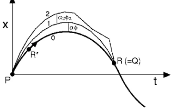
→R兲, not just at the limit ␣ = 0. We will prove this result by contradiction: assume curve

x1共t兲 共curve 1 in Fig. 10兲is not a true worldline. Consider the arbitrary comparison curve 2 in Fig. 10, which differs from 1

by the arbitrary variation ␣2␾2, with ␣2 small. Assume

共wrongly兲 that curve 1 is not a true worldline, so that the first-order variation ␦S inS between curves 1 and 2 is non-zero for arbitrary␣2␾2, and the sign of␣2 can be chosen to make S2⬍S1. But becauseS1=S0 to second order, we must have S₂⬍S₀, which is a contradiction;R is the earliest zero ofS−S0for any small variation, so that small variations giv-Fig. 10. LetRbe the earliest event along the true worldlinex₀共t兲, labeled 0, such that␦2_{S= 0 for worldlinePRalongx}

0共t兲. The unique variational func-tion achieving␦2_{S= 0 for worldline 0 corresponds to a varied curve labeled} 1. We show that for this location ofR, curve 1 is a true worldline andRis the kinetic focusQ. The arbitrary curve 2 is used to verify that curve 1 is a true worldline.

ing S−S₀⬍0 are impossible. To avoid the contradiction, curve 1 must be a true worldline. Thus we have proven that the unique variation␣␾that connectsPandR=Qwhen␦2_S goes to zero for the first time corresponds to a true worldline. This argument covers the typical case, where the integral in Eq.共20兲defining␦3S does not vanish. The only common untypical case49,57is the harmonic oscillator, which we will

discuss in Sec. VIII. The harmonic oscillator potential U

=kx2_{/ 2, for which ⳵}3_U/⳵x3 _{in Eq. 共20兲 vanishes, so that} ␦3_{S= 0 identically. Similarly, the variation} ␦4_{S and higher} variations all vanish because ⳵4U/⳵x4 and higher potential derivatives vanish. Thus for the harmonic oscillator ␦2_S=S −S0 andS−S0 remains positive up toR

⬘

=R for arbitrary ␣

共not just small ␣兲. The preceding argument with ␣→0 is

valid also for the harmonic oscillator, so that the coalescing true worldline atRagain shows thatRis the kinetic focusQ.

However, it is not necessary here to take the limit ␣→0.

Figure 3 for the harmonic oscillator shows that all true worldlines beginning atPintersect again where␦2_Sfirst van-ishes, which is the kinetic focusQ. By varying the amplitude of the alternative true worldlines for the harmonic oscillator, we can find one that coalesces with the original worldline and thus satisfies the definition of the kinetic focus. The ar-gument for other untypical cases49 is similar to that for the typical case.

In summary we have shown that as terminal eventRtakes

up positions along the worldline farther away from the initial point P, the special varied curve that leads to the earliest vanishing of␦2_{Sis typically a unique}49,58

true worldline that can coalesce with the original worldline. ThisRsatisfies the definition of the kinetic focusQ. Because the varied world-line for which␦2S= 0 for the first time is unique, it follows

that all other curves PQ adjacent to the original worldline

have␦2S⬎0.

For bound motion in a time-independent potential, world-lines that can coalesce will typically cross more than once. In the literature all of these sequential limiting crossings are called kinetic foci. The above argument is valid only for the first such crossing, which we refer to as the kinetic focus.

As we have shown, a sufficient condition for the kinetic focus Q is that it is the earliest terminal event R for which ␦2_{S= 0. In the following section we show the converse} nec-essary condition: Given the definition of the kinetic focusQ

as the first event at which a second true worldline can coa-lesce with PQ, the necessary consequence is that␦2_{S= 0 for} worldlinePQfor the variation leading to coalescence. Taken together, the arguments in these two sections prove the fol-lowing theorem, which is the fundamental analytical result of our paper:

A necessary and sufficient condition forQto be a

kinetic focus of worldlinePQ is thatQis the ear-liest event on the worldline for which␦2S= 0.

This earliest vanishing of␦2_{S occurs for one special type of} variation␣␾共which turns out to correspond to a true world-line兲, with␾unique共up to a factor兲and typically␣→0; for all other variations␦2_{Sremains positive at the kinetic focus.}

The Culverwell-Whittaker argument共more complicated than

that just given兲 is incomplete in that it addresses only the sufficiency part of the theorem 共the necessary part given in Sec. VII is new兲, and it overlooks the usual case where the limit␣→0 is necessary to locate the kinetic focus.

A simple topological picture of the action landscape in function space is emerging共see Fig. 11兲. For a short world-line PR, the action S is a minimum: the action increases in all directions away from the stationary point in function space关panel 共a兲in Fig. 11兴. For longer PR, we may reach a kinetic focusR=Qfor whichSis trough-shaped, that is, flat in one special direction and increasing in all other directions away from the stationary point 关panel 共b兲in Fig. 11兴.共The trough is completely flat for the harmonic oscillator, and flat to at least second order49for all other systems.兲As we shall

see in Sec. VII, as R moves beyond Q, the trough bends

downward, placing the action at a saddle point; that is, S

decreases in one direction in function space and increases in all other directions away from the stationary point关panel共c兲 in Fig. 11兴. Although not discussed in this paper, the pattern

may continue as R moves still further beyond the kinetic

focus Q. If R reaches a second event Q2 at which ␦2S= 0 共called the second kinetic focus in the literature兲, a trough again develops for one special variational function␾共 differ-ent from the first special ␾兲; at Q2 the action is flat in one direction in function space, decreases in one direction, and increases in all other directions. Beyond Q2 the trough be-comes a maximum, and we have a saddle point that is a maximum in two directions and a minimum in all others. Similar topological changes occur if we reach still later ki-netic foci eventsQ₃,Q₄, and so forth, a result in agreement with Morse’s theorem,34which states that the number of di-rections n in function space for which the action is a

maxi-mum at a saddle point for worldlinePRis equal to the

num-bern of kinetic foci between the end eventsP andR of the

worldline.

Fig. 11. Schematic illustration of the topological evolution of the minimum A→trough B→saddle C of the actionSfor two “directions” in function space as the final timetRincreases fromtR⬍tQtotR=tQtotR⬎tQ, respec-tively, wheretQis the kinetic focus time.共Figure adapted from Ref. 59.兲

VII. SADDLE POINT IN ACTION WHEN

WORLDLINE TERMINATES BEYOND KINETIC FOCUS

In Sec. VI we showed that a sufficient condition for the earliest event to be the kinetic focus Q is that the earliest event at which␦2S= 0 is connected to the initial eventPby a

unique true coalescing worldline. All alternative curves PQ

lead to ␦2_{S⬎0. In this section we demonstrate the} corre-sponding necessary condition, namely, given an alternative true worldline betweenPandRthat coalesces with the origi-nal worldline asR→Qand therefore definesQas the kinetic focus, we have␦2_{S= 0 for this worldline. By using an}

exten-sion of this analysis, we also show that whenRlies beyond

the kinetic focusQthe action of worldlinePQRis a saddle

point.

The essence of the proof of the first statement is outlined in the following heuristic argument by Routh.29Consider two

intersecting true worldlines P→R connecting P to R.

As-sumeRis close to the kinetic focusQso that the two world-lines differ infinitesimally, as required in the definition ofQ.

Let the action along the two worldlines be S and S+␦S,

respectively. Because both are true worldlines, the first-order variation of each is equal to zero, ␦S= 0 and ␦共S+␦S兲= 0. The difference of these two relations gives␦2S= 0 forRnear

Qand hence␦2_{S= 0 forR=Q. In the following we show that} this argument is correct in the sense that ␦2S vanishes not only atR=Q, but also vanishes toO共␣2_{兲 forR nearQ,} dif-fering from zero byO共␣3兲for RnearQ.

To make Routh’s argument rigorous, consider the two al-ternative true worldlinesx0共t兲 andx1共t兲 in Fig. 12 that con-nect the initial event P to the terminal event R, whereR is close to the kinetic focusQof x0共t兲. WhenRreachesQ, the two worldlines coalesce according to the definition of the kinetic focus Q. For definiteness, take x1共t兲 to be the top worldline in Fig. 12, which is closely adjacent to the true worldlinex₀共t兲. Hence, it is a member of the set of adjacent curves used for the variation in Sec. IV, and therefore we can employ the formalism of that section. Conversely, we can

regard x0共t兲 as a varied curve of x1共t兲, because it is closely adjacent to the other true worldline x1共t兲. Equations similar to Eqs.共5兲and共6兲are

x1共t兲=x0共t兲+␣␾共t兲, x0共t兲=x1共t兲−␣␾共t兲, 共31兲 and

x˙1共t兲=x˙0共t兲+␣␾˙共t兲, x˙0共t兲=x˙1共t兲−␣␾˙共t兲. 共32兲 We have

S₁=S₀+␦S₀+␦2S₀+␦3S₀+ ¯. 共33兲 In this case both x0共t兲 andx1共t兲 are true worldlines, so that we can also write the inverse expression

S0=S1+␦S1+␦2S1+␦3S1+ ¯. 共34兲 We subtract Eq.共34兲from Eq.共33兲and use␦S0= 0 and␦S1 = 0, because both x0共t兲 and x1共t兲 are true worldlines. The result is

2共S1−S0兲=共␦2S0−␦2S1兲+共␦3S0−␦3S1兲+ ¯. 共35兲 We then find expressions for␦2S from Eq.共19兲:

␦2_S 0=

␣2 2

冕

P

R

共−␾2U

⬙

共x0兲+m␾˙2兲dt, 共36a兲 ␦2_S

1= ␣2

2

冕

P R

共−␾2U

⬙

共x1兲+m␾˙2兲dt. 共36b兲 The first parenthesis on the right side of Eq. 共35兲 has the form

␦2_S

0−␦2S1= ␣2

2

冕

P R

dt关U

⬙

共x1兲−U

⬙

共x0兲兴␾2, 共37兲 where terms in␾˙ have cancelled. We expand U

⬙

共x1兲to first order in␣:

U

⬙

共x1兲 ⬇U

⬙

共x0兲+U

⵮共

x0兲共x₁−x0兲=U

⬙

共x0兲+U

⵮共

x0兲␣␾. 共38兲 If Eq.共38兲is substituted into Eq. 共37兲, the resulting integral contributes a further factor of␣, yielding a result ofO共␣3兲:

␦2_S

0−␦2S1⬇ ␣3

2

冕

P R

dtU

⵮共

x0兲␾3. 共39兲 The fact that the right-hand side of Eq.共39兲is proportional to␣3_{means that in Eq.共35兲we cannot neglect terms in␦}3_S that are also proportional to␣3_{.共Later terms are proportional} to ␣4 or higher.兲 From Eq. 共20兲 and the signs of ␣ in Eq. 共31兲, we have

␦3_S 0= −

␣3 6

冕

P

R

␾3_U

_⵮共

_{x0兲dt, 共40a兲}

␦3_S 1= +

␣3 6

冕

P

R

␾3_U

_⵮共

_{x1兲dt, 共40b兲}

and hence the second term on the right-hand side of Eq.共35兲 becomes

Fig. 12. By definition the kinetic focusQof the initial eventPis the first event at which two adjacent true worldlinesx0共t兲 andx1共t兲coalesce. We show that␦2_{S= 0 at the kinetic focusQfor this variational function␾in the} limitR1→Q, and that the action is a saddle point when the terminal event

R2lies anywhere on the worldline beyond the kinetic focusQ.共The lower

␣␾ has the opposite sign from the upper␣␾, and the upper and lower functions␾are slightly different due to the end-events R1 andR1⬘ being slightly different.兲