107
Job shop scheduling problem based on learning effects, flexible
maintenance activities and transportation times
Seyedhamed Mousavipour
1, Hiwa Farughi
1, Fardin Ahmadizar
11Department of Industrial Engineering, University of Kurdistan, Sanandaj, Iran
[email protected], [email protected], [email protected]
Abstract
Nowadays, scholars do their best to study more practical aspects of classical problems. Job shop Scheduling Problem (JSSP) is an important and interesting problem in scheduling literature which has been studied from different aspects so far. Considering assumptions like learning effects, flexible maintenance activities and transportation times can make this problem more close to the real life, however these assumptions have rarely been studied in this problem. This paper aims to provide a mathematical model of JSSP which covers these assumptions. MILP model is suggested, Three different sizes of instances are generated randomly, and this model has been solved for small-sized problems exactly by GAMS software and the effects of learning on reducing the value of objective function is shown. Due to the complexity of the problem, in order to obtain near optimal solutions, medium and large instances are solve by applying Ant Colony Optimization for continuous domains(ACOR) and Invasive weed Optimization (IWO) algorithm, finally results are compared.
Keywords: Job shop scheduling problem, learning effects, flexible maintenance, transportation times.
1-Introduction
The mystery that lies behind the survival of any organization is the provision of high-quality, low-price services. A factor effective on the quality and price of providing services and goods is the time when they are provided. The sequencing and scheduling of operations along the time for performing a set of jobs has been one of the concerns of decision-makers in the fields of industry and service. In today’s competitive world, efficient scheduling and sequencing is of great importance in survival of an organization in the competitive market. The problem of job shop scheduling is a versatile, important problem in the field of scheduling, considered by researchers from various aspects so far. The objective of the problem is to find an optimal scheduling where n jobs, each containing L operations, are processed on m machines, each with k positions, based on a predetermined sequence, and each job can be placed on each machine at most once. This paper seeks to present a more comprehensive and practical model of JSSP by making assumptions which have been rarely been taken into consideration in this problem, including, inter-machine transportation times, availability constraints as flexible maintenance activities and learning effects.
*Corresponding author
ISSN: 1735-8272, Copyright c 2019 JISE. All rights reserved
Journal of Industrial and Systems Engineering Vol. 12, No. 3, pp. 107- 119
108
2-Literature review
In classical scheduling, it is often assumed that the machines are always available, while they may become unavailable in the real world for certain reasons. One of these potential reasons is preventive maintenance activities planned to avoid accidental failure and to increase the useful lives of the machines. Preventive maintenance operations are of two types: fixed and flexible. In the former case, the machine becomes unavailable for performing maintenance operations after performing a number of predetermined operations, and in the latter case, the maintenance operations must be performed in a specific time window. Ma (2010) provided a comprehensive review of scheduling problems with availability constraints. Dehnar saidy and Taghavi-Fard (2008) have been studied availability constraints in different scheduling environments for both stochastic and deterministic cases. Meanwhile there are few studies on consideration of maintenance operations in the job shop environment. For example, Lei D. (2010) addressed fixed preventive maintenance operations in the fuzzy job shop problem. Lei D. (2013) investigated a multi-objective job shop problem in a nondeterministic environment by considering flexible maintenance operations, and solved it using the multi-objective artificial bee colony algorithm without presenting a mathematical model. Two-machine JSSP with predetermined maintenance activities on one machine was considered by Benttaleb et al. (2018), who presented and solved two mixed integer linear programming models using an efficient branch and bound algorithm. For minimization of makespan, a disjunctive graph model for the JSSP was presented by Tamssaouet et al. (2018) where machines are unavailable in the entire planning horizon. They used Tabu Search and Simulated Annealing for solving the problem
Vahedi Nouri et al. (2013) propose a mathematical model for flow shop scheduling problem by consideration of learning effects and flexible maintenance activities, in this study, each machine is assumed to contain a number of flexible maintenance activities, such that each maintenance activity must be done in a predetermined time window. A maintenance activity will be considered as delayed if completed later than its earliest possible finish time.
On the other hand, unlike in classical scheduling, where processing times are assumed to be fixed ,in the real production environment, repetition of a job by the operator, whether manual or semi-automatic, or of a job related to set-up in a fully-automatic environment increases the operator’s experience, and decreases operation processing times or set-up times. This phenomenon is called learning effects, first considered in scheduling problems in 1999 by Biskup. He divided learning effects into two general classes: position-based in which learning depends on the number of jobs are processed and sum-of-processing times-position-based in which processing time is considered for already-processed jobs. A large number of studies have been conducted on learning effects in single-machine and flow shop environments. Vahedi nouri et al. (2014), Amiriand and sahraeian (2015), Behnamian and Zandieh (2013), and Mousavi et al. (2018) are amongst them. Biskup (2008) and Azzur (2018) provided a comprehensive review of these studies. According to that paper, the effects of learning in the job shop environment have not yet been investigated.
Inter-machine transportation times of jobs have been ignored for simplicity in most of the studies conducted in JSSP. Transportation times can be either job-dependent or job-independent. Transportation time depends in the former case on the distance between the two machines and the job to be replaced, while it depends in the latter case only on the distance between the two machines. On the other hand, the transportation system may be multi- or single-transporter. There are an unlimited number of transporters in a multi-transporter system, while there are a limited number of them in a single-transporter system (Ahmadizar, 2014).As far as we know our paper is the first paper which considers all above mentioned assumptions together in JSSP to present a model with high compatibility with the real world.
3-Model description
In this section, assumptions, notations, parameters, scalars, decision variables and mathematical model of problem are defined:
109
3-1- Assumptions
• All jobs and machines are available at time zero. • Preemption is not allowed.
• A job cannot be processed on a machine more than once.
• Processing times of jobs are affected by classical position-based learning effects. •.The processing times include the set-up times.
• Multiple predefined flexible maintenance activities must be done on each machine. • Transportation times between machines are assumed to be job-dependent.
• Transporters don’t have any limitation.
3-2- Notations
i: Machine index j: Job index k: Position index r: Maintenance index L: Operation index
3-3-Parameters and scalars
n: Number of jobsm: Number of machines V: A large positive number
r: Number of maintenance activities performed on each machine 𝑃𝑖𝑗: Normal processing time of job 𝐽𝑗on machine 𝑀𝑖
𝑃𝑖𝑗𝑘: Processing time of job 𝐽𝑗 on the kth position of machine 𝑀𝑖
𝛼𝑖:Job processing learning index on machine 𝑀𝑖 (𝛼𝑖 ≤ 0)
𝑃𝑀𝑖𝑟:rth maintenance activity on machine 𝑀𝑖
𝐸𝐹𝑖𝑟: Earliest possible finish time of maintenance activity 𝑃𝑀𝑖𝑟
𝐿𝐹𝑖𝑟: Latest possible finish time of maintenance activity 𝑃𝑀𝑖𝑟
𝑡𝑖𝑟: Runtime of 𝑃𝑀𝑖𝑟
𝑟𝑖𝑗𝑙: A binary parameter that is 1 if the lth operation of the jth job is processed on machine𝑀𝑖, and is 0
otherwise
𝑡𝑝𝑖𝑗𝑖’:Time needed for transfer of job 𝐽𝑗 from machine 𝑀𝑖 to machine 𝑀𝑖′
3-4- Decision variables
𝑋𝑖𝑗𝑘:A binary variable that is 1 if job 𝐽𝑗 is processed on the kth position of machine𝑀𝑖, and is 0 otherwise
𝐶𝑖𝑗𝑘:Completion time of job 𝐽𝑗 if scheduled on the kth position of machine 𝑀𝑖 and 0 otherwise
𝐶𝑚𝑎𝑥: Makespan
𝑍𝑖𝑗𝑟: A binary variable that is 1 if maintenance activity 𝑃𝑀𝑖𝑟 is performed after jo𝑏𝑗 is processed on the
kth position of machine𝑀𝑖 , and is 0 otherwise
𝐹𝑀𝑖𝑟: Finish time of maintenance activity 𝑃𝑀𝑖𝑟
3-5- mathematical model
In this problem, A set of n jobs {𝐽1, 𝐽2, …, 𝐽𝑛 } each containing L operations must be processed in a
predetermined order on a set of m machines {M1, M2, …, Mm}. Each job can be processed only on one
machine at a time, and each machine can process only one job at a time. Interruption is not allowed, and there are no precedence constraints between jobs. All the jobs are available at time zero, and there are no buffer constraints between the machines. Each job 𝐽𝑗 has a predetermined normal processing time of
110
formulated by Biskup (1999). The real processing time of job 𝐽𝑗 on machine 𝑀𝑖 depends on the position
of the job in the sequence k and learning index 𝛼𝑖≤ 0, which is obtained from the equation 𝑝𝑖𝑗𝑘 = 𝑝𝑖𝑗𝑘𝛼𝑖.
Machine 𝑀𝑖 requires r maintenance activities, such that the rth maintenance operation 𝑃𝑀𝑖𝑟is completed
in a time window of [𝐸𝐹𝑖𝑟 , 𝐿𝐹𝑖𝑟] where r = 1, 2, …, r. transportation times between machines have been
taken into account as job-dependent transportation times without any limitation. Based on above mentioned assumptions, Wagner's mathematical model for JSSP has been developed to minimize makespan and sum of delays of maintenance activities as follows:
𝑀𝑖𝑛 𝑍 = 𝐶𝑚𝑎𝑥+ ∑𝑚𝑖=1∑𝑟𝑟=1(𝐹𝑀𝑖𝑟− 𝐸𝑀𝑖𝑟) (1)
(2) ∀ i = 1, … , m , j = 1, … , n
∑ 𝑋𝑖𝑗𝑘 𝑘
= 1
(3) ∀ j = 1, … , n , k = 1, … , n
∑ 𝑋𝑖𝑗𝑘 𝑗
= 1
(4) ∀ i = 1, … , m
, k = 1, … , n − 1 ∑ Cijk
j
+ ∑ Xij k+1 j
× Pij k+1≤ ∑ Cij k+1 j
(5) ∀ j = 1, … , n
, k = 1, … , n
,l= 1, … , m-1
∑ rijl i
× Cijk+ ∑ ríj l+1 í
× Xíjk× Píjk+ ∑ ∑ rijl í i
× ríj l+1× tpijí
≤ V × (1 − ∑ rijl i
× Xijk) + V
× (1 − ∑ ríj l+1 í
× Xíjk) + ∑ ríj l+1 í
× Cíjk
(6) ∀ i = 1, … , m
, j = 1, … , n , r = 1, … , r ∑ Cijk
k
− ∑ Xijk k
× Pijk − 𝐹𝑀𝑖𝑟+ 𝑍𝑖𝑗𝑟× v ≥ 0
(7) ∀ i = 1, … , m
, j = 1, … , n , r = 1, … , r 𝐹𝑀𝑖𝑟− 𝑡𝑖𝑟+ 𝑉(1 − 𝑍𝑖𝑗𝑟) ≥ ∑ 𝐶𝑖𝑗𝑘
𝑘
(8) ∀ i = 1, … , m
, j = 1, … , n 𝐶𝑖𝑗𝑘 ≤ 𝑉 × 𝑋𝑖𝑗𝑘
111
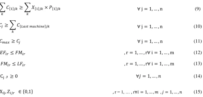
(9) ∀ j = 1, … , n
∑ 𝐶[1]𝑗𝑘 𝑘
≥ ∑ 𝑋[1]𝑗𝑘 𝑘
× 𝑃[1]𝑗𝑘
(10) ∀ j = 1, … , n
𝐶𝑗 ≥ ∑ 𝐶[𝐿𝑎𝑠𝑡 𝑚𝑎𝑐ℎ𝑖𝑛𝑒]𝑗𝑘 𝑘
(11) ∀ j = 1, … , n
𝐶𝑚𝑎𝑥 ≥ 𝐶𝑗
(12) ∀ i = 1, … , m
, r = 1, … , r 𝐸𝐹𝑖𝑟≤ 𝐹𝑀𝑖𝑟
(13) ∀ i = 1, … , m
, r = 1, … , r 𝐹𝑀𝑖𝑟 ≤ 𝐿𝐹𝑖𝑟
(14) ∀𝑗 = 1, … , 𝑛
Cj و ≥ 0
(15) ∀𝑖 = 1, … , 𝑚 , 𝑗 = 1, … , 𝑛
,r = 1, … , r X𝑖j, 𝑍𝑖𝑗𝑟 ∈ {0,1}
In this model, the first equation is the objective function to minimize makespan and sum of delays of maintenance activities. Constraints 2 and 3 state that each job can assign to one position and each position can involve one job. Constraint 4, calculates completion time of jobs on each position of machines regarding to learning effects. Constraint 5 is the precedence constraint and considers transportation times, Constraints 6 and 7 determine finish time of maintenance activities. Constraint 8 express that the completion time of job 𝐽𝑗 is 1 if it is scheduled in the kth position of machine 𝑀𝑖, and is 0 otherwise;
constraints 9-11 compute completion time of each job and makespan as well. Constraints 12 and 13 indicate time window for each maintenance activity. Finally two last constraints reveal positive and binary variables.
4-Data generation
Due to the novelty of the proposed model and lack of benchmarks in the literature, three types of problems in small, medium, and large sizes are randomly generated. If a, b, and c represent the number of machines, jobs, and maintenance operations, respectively, the borders of these three groups have been considered 30 and 60 regarding to the CPU times of solution methods which have been gained by trial and error. In this way, small-sized problems lie in the range a.b.c ≤ 30, Medium-sized problems lie in the range 30 ≤ a.b.c ≤ 60, and a.b.c > 60 in large-sized problems. Table 1 illustrates the quality of data generation for random instances. It is worth mentioning that formulations for 𝐸𝐹𝑖𝑟 and 𝐿𝐹𝑖𝑟 have been
generated by trial and error, based on vahedi-Nouri et al. (2013).
Table 1. Data Generation
parameter Notation Value
n Number of jobs {2…12}
m Number of machines {3…14}
r Number of maintenance on each machine 2
𝛼𝑖 Learning index of machine Mi Uniform distribution(-0.9 , -0.1)
𝑡𝑖𝑟 maintenance execution time Uniform distribution(5,35)
𝐸𝐹𝑖𝑟 Earliest possible finish time of
maintenance activity 𝑃𝑀𝑖𝑟
K(∑𝑛𝑗=1𝑃𝑖𝑗) ∕ (k+1) + 30(i-1)
𝐿𝐹𝑖𝑟 Latest possible finish time of maintenance
activity 𝑃𝑀𝑖𝑟
K(∑𝑛𝑗=1𝑃𝑖𝑗) ∕ (k+1) + 30(i)
𝑡𝑝𝑖𝑗𝑖′ Transportation times Uniform distribution (1,40)
112
5-Proposed solution methods
Since the JSSP is a strongly NP-hard problem, the presented MILP model is solved using the solver of CPLEX of GAMS 24.8.5 for small-sized problems, and two metaheuristic algorithms are applied for finding near-optimal solutions in medium and large-sized problems, where the exact methods are incapable of finding optimal solutions within logical time. MATLAB 2015 and a PC with a Core i5 2.5GHz CPU, 3MB cache, and 4GB RAM have been used for coding these algorithms.
5-1- metaheuristic algorithms
To handle medium and large instances, two metaheuristic algorithms i.e. ACOR which is Ant Colony Optimization (ACO) algorithm extended for continuous domains and Invasive Weed Optimization (IWO). The ant colony algorithm was introduced by Colorni et al. (1992). It is a population-based metaheuristic that can find near-optimal solutions in complex hybrid optimization problems based on the behavior patterns of ants. For the algorithm to be utilized, artificial ants progressively generate solutions by moving on the graphs. The process of generating solutions is random, and is biased using the pheromone model. The algorithm uses a discrete structure for specification of solutions. That is, each of the decision variables is divided into a specific number of modes in the defined range. The discretization of the variable space restricts the algorithm, which in turn reduces its accuracy. Bilchev and Parmee (1995), proposed the ACOR algorithm. A probability density function (PDF) is used in the algorithm to make the space continuous in the decision variables. Mehrabian and Lucas (2006) introduced a random optimization algorithm inspired by colonizing weeds. They state that weeds are wild plants with aggressive growth habits, which makes them a serious threat to desired plants, disordering agriculture. They have indicated the great capability of adaptation to the environment and stability. IWO algorithm seeks to present a simple, efficient method for solving problems by imitating the stability, adaptation, and random behavior in the weed colony. Noteworthy is to mention that parameters of these algorithms have been tuned by trial and error. Figure1 shows flowchart of IWO
5-2- Solution representation
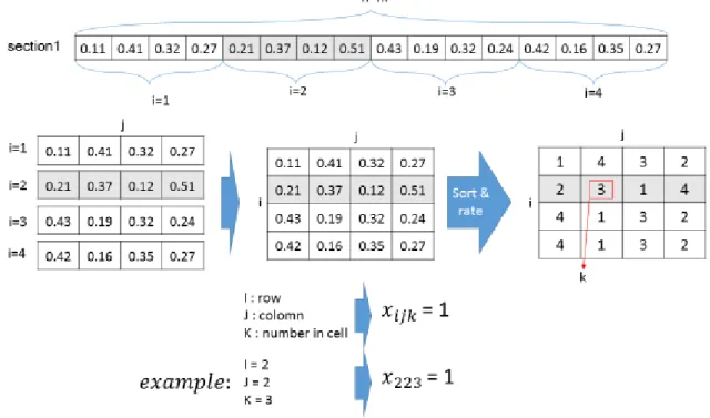
JSSP is a NP-hard problem (Fattahi, 2017). A dimension which is added to it by the learning effects makes it more complicated. Therefore, we should seek for appropriate and efficient solution methods to solve medium and large instances. In this way, a string of decimal numbers is used for presentation of the solution. The solution representation should represent only one solution to the problem. The string is as long as "the number of machines" × "the number of jobs". Each string is divided into number of machines, and each section is arranged in ascending order. In each section, the sequence of jobs that each machine is assigned is specified by the sequence of arranged numbers for that machine. Figure 2 demonstrates this procedure.
113
Fig 1. Flowchart of IWO (Velmurugan, 2016)
114
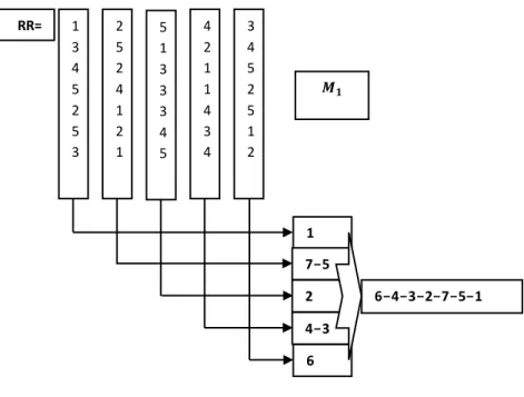
Noteworthy is to mention that, for gaining the feasible solutions, an initial solution for the problem is created at the beginning of the algorithm with a heuristic method that generates the first feasible solution for each machine greedily. Figure 3 depicts this procedure.
Fig 3. Generating an initial solution
(Sequence of jobs processed on machine M1)
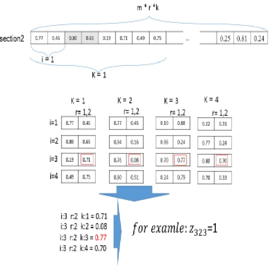
As figure 4 Depicts, The following section of the solution representation of length "the number of machines" × "the number of maintenance activities" × "the number of positions" concerns specification of maintenance operations r performed at position k after processing 𝐽𝑗on machine 𝑀𝑖. Here, the highest
value of k is specified for every machine and maintenance activity. This value of k specifies where the maintenance operations are performed on the machine.
6-Comparison of the solutions
To compare the solution methods, three metrics have been applied. The first one is Relative Percentage Deviation (RPD). Equivalent RPD of each solution is calculated by equation (16), where 𝐴𝑙𝑔𝑠𝑜𝑙the
objective value is obtained by solving an instance using the considered solution method, and 𝑀𝑖𝑛𝑠𝑜𝑙 is
the minimum objective value obtained by solving that instance using solution methods. The value of RPD for each solution method shows the ability of solution method to find more appropriate solutions such that the less value of RPD indicates that solution method has been managed to find the less value of objective function. Furthermore, Imp (Improvement) as the second metric indicates the amounts of improvement occurred in the initial solution, obtained by equation (17), where 𝐴𝑙𝑔𝑖𝑛𝑖𝑡𝑖𝑎𝑙𝑠𝑜𝑙 is the objective value of the
initial solution of the solution method, and 𝐴𝑙𝑔𝑓𝑖𝑛𝑎𝑙𝑠𝑜𝑙 is the objective value of its final solution. CPU
time of each solution method is the third metric for comparison the efficiency of each method. RPD =𝐴𝑙𝑔𝑠𝑜𝑙−𝑀𝑖𝑛𝑠𝑜𝑙
𝑀𝑖𝑛𝑠𝑜𝑙 × 100 (16)
Imp =𝐴𝑙𝑔𝑖𝑛𝑖𝑡𝑖𝑎𝑙𝑠𝑜𝑙−𝐴𝑙𝑔𝑓𝑖𝑛𝑎𝑙𝑠𝑜𝑙
𝐴𝑙𝑔𝑖𝑛𝑖𝑡𝑖𝑎𝑙𝑠𝑜𝑙 × 100 (17)
1 3 4 5 2 5 3 2 5 2 4 1 2 1 5 1 3 3 3 4 5 4 2 1 1 4 3 4 3 4 5 2 5 1 2 1 5 -7 6 3 -4
2 6-4-3-2-7-5-1 RR=
115
Fig 4. Determining the position of maintenance activity
7-Computational results
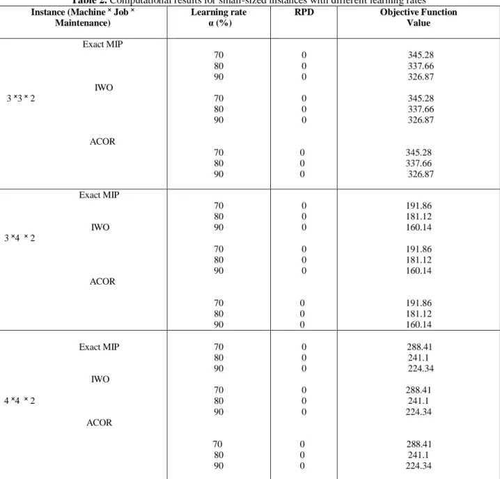
To validate the model and investigate the effects of learning on the objective function value and to ensure that metaheuristic methods function correctly, four small-sized examples are solved using GAMS and metaheuristic methods at three different rates of learning, and the results are shown in table 2.
116
Table 2. Computational results for small-sized instances with different learning rates
As table 2 shows the values of RPD for exact and metaheuristic methods are 0, consequently the ability of ACOR and IWO is confirmed to obtain optimal solutions for small problems, moreover we are convinced about the validity of these algorithms to find near optimal solutions for medium and large problems. On the other hand results indicate that by increasing the learning rate, the value of objective function is reduced, it means that the more learning in environment can decrease the value of objective function and improve the productivity
.
Instance (Machine ˟ Job ˟ Maintenance)
Learning rate α (%)
RPD Objective Function Value
Exact MIP IWO 3 ˟3 ˟ 2
ACOR 70 80 90 70 80 90 70 80 90 0 0 0 0 0 0 0 0 0 345.28 337.66 326.87 345.28 337.66 326.87 345.28 337.66 326.87 Exact MIP IWO
3 ˟ 4 ˟ 2
ACOR 70 80 90 70 80 90 70 80 90 0 0 0 0 0 0 0 0 0 191.86 181.12 160.14 191.86 181.12 160.14 191.86 181.12 160.14 Exact MIP IWO
4 ˟ 4 ˟ 2
ACOR 70 80 90 70 80 90 70 80 90 0 0 0 0 0 0 0 0 0 288.41 241.1 224.34 288.41 241.1 224.34 288.41 241.1 224.34
117
Table 3. Computational results for medium and large instances
IWO ACOR
Representation RPD CPU time
(s)
Imp RPD CPU time
(s)
Imp
4 × 5 × 2 0 153.152 0.141 0 226.77 0.136
5 × 5 × 2 0 186.45 0.188 0.0003 234.26 0.187
5 × 6 × 2 0 198.63 0.09 0.0130 287.34 0.276
6 × 7 × 2 0 206.45 0.283 0.0486 337.45 0.30
8 × 9 × 2 0 217.69 0.4284 0.115 362.72 0.392
10 × 9 × 2 0 726.54 0.470 0.0895 1085.23 0.563
12 × 10 × 2 0 809.55 0.373 0.102 1261.08 0.454
14 × 12 × 2 0 965.43 0.410 0.179 1636.54 0.437
Mean 0 409.70 0.297 0.0683 678.91 0.343
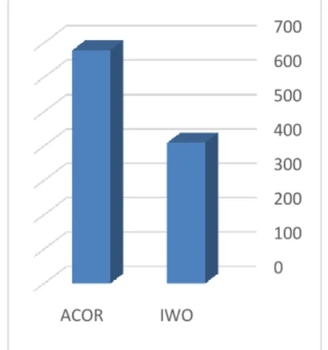
Table 3 shows the results of solving model by IWO and ACOR for 8 medium and large instances. Figure 5 illustrates mean CPU times for these instances, as this figure shows IWO enjoy less CPU time. As figure 6 reveals, regarding to the mean values of RPD, both algorithms find semi same results but IWO can find rather better solutions, although difference between mean RPD of IWO and ACOR is less than 1 percent. As figure7 demonstrates ACOR create more improvement in proportion to the initial solution, this difference is less than 0.05.
Fig 5. "Mean CPU times" for IWO and ACOR Fig. 6- Mean values of "RPD" for IWO and ACOR
Fig 7. Mean values of "Imp" for IWO and ACOR
0 100 200 300 400 500 600 700
IWO ACOR
0 0.01 0.02 0.03 0.04 0.05 0.06 0.07
IWO ACOR
0.27 0.28 0.29 0.3 0.31 0.32 0.33 0.34 0.35
IWO ACOR
118
8-Conclusion
In this paper a novel position-based model has been suggested for the JSSP in which practical assumptions contain learning effects, flexible maintenance activities and transportation times have been taken into account. We have shown that consideration of learning effects can improve objective function and consequently production costs can be reduced. Proposed MILP model has been solved in small scale by GAMS software moreover for solving this model in large scale two metaheuristic algorithms i.e. Invasive Weed Optimization (IWO) and Ant Colony Algorithm for continues domains (ACOR) have been applied, finally results have been compared based on three metrics, and meanwhile IWO can gain better results mildly. For future researches, considering issues like sequence –dependent set up times, other types of learning effects and fixed maintenance activities in JSSP and other production environments can be appealing.
References
Amirian, H., Sahraeian, R. (2015). Augmented ε-constraint method in multi-objective flow shop problem with past sequence set-up times and a modified learning effect. International Journal of Production Research ,53 (19), 1-15.
Ahmadizar, F., Shahmaleki, p. (2014). Group-shop scheduling with sequence-dependent set-up and transportation times, Applied Mathematical Modelling, 38(21) 5080-5091.
Azzouz, A., Ennigrou, M., & Ben Said, L. (2018). Scheduling problems under learning effects: classification and cartography, International Journal of Production Research, 56(4), 1642–1661.
Behnamian, J., Zandieh,M.(2013). Earliness and Tardiness Minimizing on a Realistic Hybrid Flowshop Scheduling with Learning Effect by Advanced Metaheuristic, Arab J Sci Eng 38, 1229–1242 .
Benttaleb, M., Hnaien, F., & Yalaoui, F. (2018). Two-machine job shop problem under availability constraints on one machine: Makespan minimization; Computers & Industrial Engineering 117, 138–151. Bilchev, G., Parmee, I. (1995). The Ant Colony Metaphor for Searching Continuous Design Spaces. In Fogarty, T.C., and ed.: Evolutionary Computing. AISB Workshop. Springer, Sheffield, UK: 25–39. Biskup, D. (1999). Single-machine scheduling with learning considerations, European Journal of Operational Research, 115 (1), 173–178.
Biskup, D. (2008). A state-of-the-art review on scheduling with learning effect, European Journal of Operational Research, 188(2), 188 – 315.
Colorni, Am., Dorigo, M., Maniezzo, V (1992). Distributed Optimization by Ant Colonies. EUROPEAN CONFERENCE ON ARTIFICIAL LIFE, PARIS, FRANCE, ELSEVIER PUBLISHING, 134–142. Dehnar saidy, H., Taghvi-Fard, M. (2008). Study of Scheduling Problems with Machine Availability Constraint. Journal of Industrial and Systems Engineering Vol. 1, No. 4, pp 360-383.
Fattahi, p, Daneshamooz, F. (2017). Hybrid algorithms for job shop scheduling problem with lot streaming and a parallel assembly stage. Journal of Industrial and Systems Engineering, 10(3), 92-112.
119
Lei, D., (2010). Fuzzy job shop scheduling problem with availability constraints. Computers & Industrial Engineering 58, 610–617.
Lei, D., (2013). Multi-objective artificial bee colony for interval job shop scheduling with flexible maintenance, Int J Adv Manuf Technol 66, 1835–1843.
Ma, Y., Chu, C., & Zuo, C. (2010). A survey of scheduling with deterministic machine availability constraints. Computers & Industrial Engineering, 58(2), 199–211.
Mehrabian, A.R., Lucas, C. (2006). A novel Numerical Optimization Algorithm Inspired from Weed Colonization, Ecological Informatics, 1,.355- 366.
Mousavi,S.M., Mahdavi,L., Rezaeian, J., Zandieh,M. (2018). Bi-objective scheduling for the re-entrant hybrid flow shop with learning effect and setup times;Scientia Iranica E 25(4), 2233-2253.
Tamssaouet, K., Dauzère-Pérès, S., & Yugma, C. (2018). Metaheuristics for the job-shop scheduling problem with machine availability constraints; Computers & Industrial Engineering 125: 1–8.
Vahedi-Nouri, B., Fattahi, P., & Ramezanian, R. (2013). Hybrid firefly-simulated annealing algorithm for the flow shop problem with learning effects and flexible maintenance activities, International Journal ofProduction Research, 51(12), 3501-3515.
Vahedi-Nouri, B., Fattahi, P., Tavakkoli-Moghaddam, R., and Ramezanian, R. (2014). A general flow shop scheduling problem with consideration of position-based learning effect and multiple availability constraints, International Journal of Advanced Manufacturing Technology, 73 (5) ,601–611 (2014). Velmurugan,T., Sibaram, k., Nadakumar,S., Saravanan,B. (2016). Seamless Vertical Handoff usingInvasive Weed Optimization (IWO) algorithm for heterogeneous wireless networks. Ain Shams Engineering journal, 7(1), 101-111.
Wagner, H.M. (1959). An integer linear-programming model for machine scheduling, Naval Rest Logis Q, 6 (2), 131–40.