Design and Implementation of Stewart Platform Robot for Robotics Course Laboratory

DESIGN AND IMPLEMENTATION OF STEWART PLATFORM ROBOT FOR ROBOTICS COURSE LABORATORY

A Thesis

presented to

the Faculty of California Polytechnic State University,

San Luis Obispo

In Partial Fulfillment

of the Requirements for the Degree

Master of Science in Mechanical Engineering

by

Trent Robert Peterson

©2020

COMMITTEE MEMBERSHIP

TITLE: Design and Implementation of Stewart Platform Robot for Robotics Course Lab-oratory

AUTHOR: Trent Robert Peterson

DATE SUBMITTED: March 2020

COMMITTEE CHAIR: Saeed B. Niku, Ph.D.

Professor of Mechanical Engineering

COMMITTEE MEMBER: William R. Murray, Ph.D.

Professor of Mechanical Engineering

COMMITTEE MEMBER: John R. Ridgely, Ph.D.

ABSTRACT

Design and Implementation of Stewart Platform Robot for Robotics Course Laboratory

Trent Robert Peterson

A Stewart Platform robot was designed, constructed, and programmed for use in Cal Poly’s ME 423 Robotics: Fundamentals and Applications laboratory section. A Stewart Platform is a parallel manipulator robot with six prismatic joints that has six degrees of freedom, able to be defined in both position and orientation. Its purpose is to supplement parallel robot material covered in lecture. Learning objectives include applying and verifying the Stewart Platform inverse kinematics and investigating the Stewart Platform’s operation, range of motion, and limitations. The Stewart Plat-form geometry and inverse kinematics were modeled and animated using MATLAB. The platform was then built using linear actuators, magnetic spherical bearings, and acrylic plates. Control of the Stewart Platform is achieved using an Arduino Due and a custom HexaMoto shield. Users interact with the system using a GUI created with MATLAB’s App Designer.

ACKNOWLEDGMENTS

I would like to thank Dr. Saeed Niku for providing me the opportunity to create a robot and give back to the university, and for the guidance and patience along the way.

I would like to thank the members of my thesis committee, Dr. William Murray and Dr. John Ridgely, for imparting onto me the knowledge to make this robot and thesis possible.

I would like to thank Charlie Refvem for reviewing my board and giving me advice as I assembled my electronics hardware, saving me lots of time and potentially wasted effort.

I would like to thank the Cal Poly Mechanical Engineering Department for funding this robot, and to Christine Haas for working with me through the process.

I would like to thank Progressive Automations for the (pending) donation of the linear actuators.

I would like to thank Helical Products Company for supplying flexible couplings for use with the robot.

TABLE OF CONTENTS

Page

LIST OF TABLES . . . x

LIST OF FIGURES . . . xi

CHAPTER 1 Introduction and Background . . . 1

1.1 Robots: A General Overview . . . 1

1.2 Parallel Robots . . . 2

1.2.1 Advantages and Disadvantages . . . 3

1.3 Stewart Platform . . . 4

1.3.1 Geometry Stability . . . 5

1.3.2 History . . . 6

1.3.3 Kinematic Equations . . . 7

1.3.4 Applications . . . 12

1.3.5 Stewart Platform Specifications . . . 13

2 Mechanical Design . . . 15

2.1 Linear Actuators . . . 15

2.1.1 Selection Guidelines . . . 18

2.1.2 Progressive Automation PA-14P-8-35 . . . 18

2.2 Magnetic Spherical Joints . . . 19

2.3 Platform Material . . . 21

2.4 Shaft Couplers . . . 22

2.5 6-3 Configuration Geometry . . . 24

3 Electronic Design . . . 29

3.1 Microcontroller - Brief Overview . . . 30

3.1.1 Microcontroller Selection . . . 30

3.1.2 Arduino Due Specifications . . . 32

3.2 HexaMoto Shield . . . 33

3.2.1 Design Requirements . . . 34

3.2.2 Robot Power’s MultiMoto Arduino Shield . . . 35

3.2.3 HexaMoto Design . . . 36

3.2.4 Component Details . . . 38

3.2.4.1 STMicroelectronics L9958SBTR Motor Driver . . . . 38

3.2.4.2 I/O Hardware Components . . . 40

3.3 HexaMoto Shield Assembly . . . 40

3.4 DC Power Supply . . . 42

3.5 Connectors . . . 43

3.6 Electrical Assembly and Integration . . . 45

4 Software Design . . . 47

4.1 Matlab Platform Simulation . . . 47

4.1.1 Geometrical Properties . . . 47

4.1.2 Motion Profile . . . 49

4.1.3 Calculation and Animation . . . 50

4.2 Arduino Sketch . . . 52

4.2.1 Arduino Sketch Source Credit . . . 53

4.2.2 Setup and Initialization . . . 54

4.2.3 Calibration and Homing . . . 54

4.3.1 Serial Connection . . . 56

4.3.2 Platform Configuration . . . 56

4.3.3 Linear Actuator Position Calculation . . . 57

4.3.4 Saving and Sequencing Points . . . 58

4.3.5 Motion . . . 59

5 Testing and Future work . . . 60

5.1 Testing . . . 60

5.2 Conclusion . . . 64

5.3 Improvements . . . 64

5.3.1 HexaMoto Shield . . . 64

5.3.2 Acrylic Plates . . . 65

5.4 Future Work . . . 66

6 Lab Manual . . . 68

6.1 Lab Manual . . . 68

6.2 Learning Objectives . . . 68

BIBLIOGRAPHY . . . 69

APPENDICES A PA-14P Datasheet . . . 71

B WAC20-4mm-4mm Datasheet . . . 79

C Mechanical Drawings . . . 81

D Mechanical Bill of Materials . . . 90

E MultiMoto Schematic . . . 91

F HexaMoto Schematic . . . 94

G Electrical Bill of Materials . . . 97

I Matlab Simulation Script . . . 105

J Arduino Sketch . . . 117

K Matlab GUI Code . . . 123

LIST OF TABLES

Table Page

1.1 Stewart Platform Specifications . . . 14

2.1 Magnetic Spherical Joint Product Options [1] . . . 20

3.1 Arduino Due Technical Specifications [3] . . . 32

4.1 Inverse Kinematics Solution for 6-6 Configuration . . . 52

5.1 Commanded and Actual Actuator Lengths . . . 60

5.2 Stewart Platform Positional Test Measurements . . . 61

LIST OF FIGURES

Figure Page

1.1 Closed and Open Kinematic Loop Mechanisms . . . 2

1.2 Stewart Platform Configurations . . . 4

1.3 Typical Stewart Platform Joint Configuration . . . 5

1.4 Unstable 6-6 Configuration . . . 6

1.5 Tire Testing Machine Application of Stewart Platform [13] . . . 7

1.6 Home Position of Stewart Platform Robot . . . 8

1.7 AMiBA Radio Telescope in Hawaii [12] . . . 13

2.1 Section View of an Electric Linear Actuator [10] . . . 17

2.2 Ball Joint Rod Ends [14] . . . 19

2.3 Magnetic Spherical Joint Properties . . . 21

2.4 Helical WAC20mm-4mm-4mm Couplings . . . 23

2.5 Range-of-Motion Limitation with Sharing Spherical Joint . . . 24

2.6 Range-of-Motion Limitation with Sharing Spherical Joint . . . 25

2.7 Joint Angle of Spherical Joint in 6-3 Configuration . . . 25

2.8 Electronic Enclosure . . . 27

2.9 Arduino Due Mount . . . 27

2.10 Molex Connector Retainer and Label . . . 28

3.1 Stewart Platform System Diagram . . . 29

3.2 Arduino Due [3] . . . 32

3.3 Progressive Automation PA-14P Pinout [19] . . . 35

3.5 HexaMoto Board Layout, Top Layer . . . 37

3.6 L9958 Block Diagram and PowerSO16 Pinout [22] . . . 38

3.7 L9958 Application Circuit [22] . . . 39

3.8 SunLED Bi-Directional LED [9] . . . 39

3.9 HexaMoto Shield I/O Hardware . . . 40

3.10 HexaMoto Shield, Post Solder Paste Application and Reflow . . . . 41

3.11 HexaMoto Shield, Completed . . . 42

3.12 PA-14P Current Draw vs Load [19] . . . 43

3.13 Power and USB Receptacle Connectors Enclosure . . . 44

3.14 MicroUSB to USB-B Connector . . . 44

3.15 Painted Electronic Enclosure with PSU and Connectors . . . 45

3.16 Enclosure Wiring . . . 46

4.1 Animation Screenshots . . . 47

4.2 Motion Profile Creation . . . 49

4.3 Matlab Simulation Plots for Joint Values . . . 50

4.4 Matlab Simulation Plots for Orientation Values . . . 51

4.5 6-6 Configuration Model for Inverse Kinematics Solution . . . 51

4.6 Arduino State Transition Diagram . . . 53

4.7 Matlab GUI for Stewart Platform . . . 55

4.8 Serial Connection and Calibration . . . 56

4.9 Top and Bottom Joint Locations . . . 57

4.10 Position and Orientation Input . . . 57

4.11 Save and Sequence Panel . . . 58

Chapter 1

INTRODUCTION AND BACKGROUND

1.1 Robots: A General Overview

A robot is a machine that can be easily commanded, typically by a computer, to perform a set of tasks automatically. Robots are extraordinarily diverse in size, performance, cost, and operation. They typically have multiple links and actuators that create kinematic chains, and connect to an end effector. An end effector is a tool that is connected to the end of a robotic mechanism. The end effector may move in space in up to six ways called degrees of freedom (DOF). Three degrees of freedom are translation which occur along mutually-orthogonal axes, typically referred to as X, Y, and Z. Another three DOF may be rotation, which occur about these three axis. These six DOF are necessary to completely define the position and orientation of an object in space.

accurately is more difficult. Links are rigid members that connect the joints of a robot.

Forward kinematics and inverse kinematics are an integral segment of robotic study and analysis. Forward kinematics allows the position and orientation of the end effector to be known, given all joint values. Inverse kinematics determines the joint values given a known or desired end effector position and orientation.

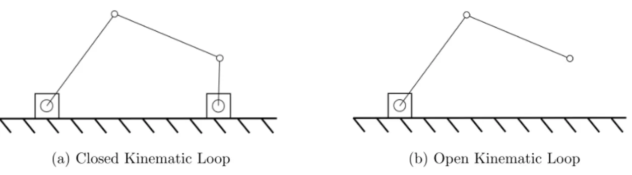
The combination of joints and links comprise a kinematic loop, which can be either closed or open. An open kinematic loop occurs when links are connected in serial form via joints. The kinematic loop is closed when each link, which includes ground, is connected to a minimum of two other links. A four-bar linkage is a common mechanism that has a closed kinematic loop. The arm of an excavator is an example of an open loop mechanism (Figure 1.1).

(a) Closed Kinematic Loop (b) Open Kinematic Loop Figure 1.1: Closed and Open Kinematic Loop Mechanisms

1.2 Parallel Robots

geometry gives a parallel robot its distinct characteristics, analysis, and behavior. Parallel robots can have up to six DOF and have various constructions.

1.2.1 Advantages and Disadvantages

It is important to compare the differences between serial and parallel robots and illustrate the areas in which each type of robot excels. An important characteristic of a robot is its payload-to-mass ratio, which is typically higher for parallel robots. This is due to the closed-loop construction of a parallel robot. By distributing the loading of the robot between its actuators, this construction supports greater forces that comes with increased mass or acceleration. In comparison, the open-loop construction of a serial robot successively increases the load seen by each joint. The outermost joint, the wrist, needs to support the mass and inertial forces from the end effector only. The next joint, the elbow, must support the end effector, the wrist joint, and the forearm link. This continues to the base of the robot. Loading of an open-loop mechanism can cause deformation that is not detected by sensors which reduces positional accuracy. To compensate, the serial robot must be made very stiff, and this over-designed geometry increases robot weight. High stiffness and payload-to-mass ratios in parallel robots is generally accompanied by a reduction in workspace compared to similarly-sized serial robots.

1.3 Stewart Platform

The Stewart Platform is a common type of parallel manipulator and possesses six degrees of freedom. In their paper, Cruz, Ferreira, and Sequeira [5] state that “the generic Stewart-Gough platform is composed of two rigid bodies connected through a number of prismatic actuators as in a parallel arrangement of kinematic chains. Usually six actuators are used, pairing arbitrary points in the two bodies.”

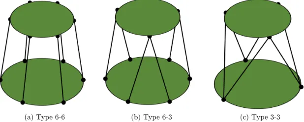
The actuators are connected to the rigid bodies by spherical or universal joints. This would mean the Stewart Platform is a spherical-prismatic-spherical, or SPS, robot. Although the joint positions can be arbitrary, evenly spacing them results in special cases. When the joints are spaced 60°around the base and the moving platform, this is called a 6-6 configuration. When a pair of actuators share the same joint spaced 120° on the moving platform, this is called a 6-3 configuration. 120° spacing on top and bottom platforms results in a 3-3 configuration as shown in Figure 1.2.

(a) Type 6-6 (b) Type 6-3 (c) Type 3-3

1.3.1 Geometry Stability

In a literature survey, a true type 6-6 Stewart Platform was never found to be used in practice. Typically, platforms were designed as a mix between the 6-6 and 3-3 configuration. Instead of pairs of actuators sharing the same joint, each actuator had its own joint like in a 6-6 configuration; pairs of joints were separated by a small gap, resulting in a geometry visually similar to Type 3-3. A diagram of this geometry is shown in Figure 1.3 and example platforms are shown in Section 1.3.4.

Figure 1.3: Typical Stewart Platform Joint Configuration

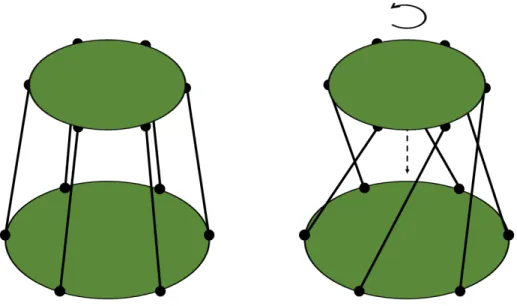
Figure 1.4: Unstable 6-6 Configuration

1.3.2 History

the platform has become known as the Stewart-Gough Platform, or more informally as the Stewart Platform.

Figure 1.5: Tire Testing Machine Application of Stewart Platform [13]

1.3.3 Kinematic Equations

The Stewart Platform kinematics are derived from analysis of its six kinematic chains. The following derivation is drawn from Dr. Saeed Niku’s inverse kinematic derivation of the Stewart Platform, found in the 3rd edition of his book,Introduction to Robotics:

Figure 1.6: Home Position of Stewart Platform Robot

A fixed reference framexyz is placed at the center of the platform base. Thez-axis is normal to the base and the x-axis is parallel to it, pointed towards a spherical joint. A moving reference framenoa is similarly placed at the center of the moving platform with thea-axis normal to the moving platform face and then-axis pointed towards a spherical joint. The spherical joints are assumed to be connected through the linear actuator. Frame noa rotates by θ,φ,ψ respectively.

Four parts compose each kinematic chain C: A connects the origin of the fixed reference frame and base spherical joint at an angle from x. B connects the origin of the moving reference frame and moving platform spherical joint at an angle from

Li =P +Bi−Ai (1.1)

for i = 1..6.

For chainC1,A1 and B1 lie along thex-axis andn-axis respectively and their angles

are zero. In a Type 6-6 Stewart Platform, subsequent chains will be multiples of 60° from thex and n axes. This is not always the case, and the remaining angles can be arbitrary values; in practice, Stewart Platforms will have some degree of symmetry.

Following the vector convention of Introduction to Robotics by Dr. Saeed Niku [16],

Ai for the general case can be written as

Ai =

        

Acos(ith)

Asin(ith)

0 1          (1.2)

where the ith term is the angle that Ai makes with the x axis.

Ai for i=1..6 will remain constant throughout the motion of the Stewart Platform for

a given geometry.

Similarly, Bi can be written as

Bi =

        

Bcos(ith)

Bsin(ith)

for the moving platform when it is in the home position as shown in Figure 1.6. The home position is achieved after the robot is calibrated, and all the actuators are at their minimum length.

Because Bi is attached to moving frame noa, its components will change as the

plat-form rotates. To account for this rotation, Bi must be pre-multiplied by rotation

matrices. Using the variables from the moving reference frame, the rotation matrices are:

Rot(x, θ) =

     

1 0 0

0 cosθ −sinθ

0 sinθ cosθ

      (1.4)

Rot(y, φ) =

     

cosφ 0 sinφ

0 1 0

−sinφ 0 cosφ

      (1.5)

Rot(z, ψ) =

     

cosψ −sinψ 0

sinψ cosψ 0

0 0 1

      (1.6)

Equations 1.4, 1.5, and 1.6 are from equations 2.20 and 2.21 inIntroduction to Robotics

[16]. These 3x3 rotation matrices only account for rotation. They can be expanded to 4x4 to include position, in which the fourth row and column are zero, except for a value of one located in element 4,4.

In order to determine the value ofBi after rotation for each kinematic chain, it must

        

Bix

Biy

Biz

1          rot =

Rot(z, ψ) Rot(y, ψ) Rot(x, θ)

        

Bix

Biy

Biz

1          home (1.7)

Multiplying Rot(z, ψ) andRot(y, φ) yields

Rot(z, ψ) Rot(y, ψ)

=      

cosφcosψ −sinψ cosψsinφ

cosφsinψ cosψ sinφsinψ

−sinφ 0 cosφ

      (1.8)

Multiplying the result of Equation 1.8 by Rot(x, θ) yields

     

cosφcosψ −sinψ cosψsinφ

cosφsinψ cosψ sinφsinψ

−sinφ 0 cosφ

           

1 0 0

0 cosθ −sinθ

0 sinθ cosθ

      =      

cosφcosψ cosψsinφsinθ−cosθsinψ sinψsinθ+cosψcosθsinφ

cosφsinψ cosψcosθ+sinφsinψsinθ cosθsinφsinψ−cosψsinθ

−sinφ cosφsinθ cosφcosθ

      (1.9)

After combining the rotation matrices, Equation 1.7 becomes

        

Bix

Biy

Biz 1          rot =         

cosφcosψ cosψsinφsinθ−cosθsinψ sinψsinθ+cosψcosθsinφ 0 cosφsinψ cosψcosθ+sinφsinψsinθ cosθsinφsinψ−cosψsinθ 0

−sinφ cosφsinθ cosφcosθ 0

0 0 0 1

                 

Bix

Biy

[Bi]home is known from the Stewart Platform geometry, and θ, φ, and ψ are known

upon specifying the orientation of the moving platform. Therefore, [Bi]rot can be

solved. Expanding the vectors Equation 1.1 into component form yields

      Lix Liy Liz       =       Pix Piy Piz       +       Bix Biy Biz       −       Aix Aiy Aiz       (1.11) for i=1..6.

The linear actuator lengths are the desired quantity from the kinematics. The mag-nitude of each length is determined by

|Li|=

q

(Lix)2+ (Liy)2+ (Liz)2 (1.12)

for i=1..6.

These calculated lengths become the setpoints for controlling the Stewart Platform.

1.3.4 Applications

properly. In astronomy, Stewart Platforms are used in spherical radio telescopes and trajectory tracking, such as the one shown in Figure 1.7.

Figure 1.7: AMiBA Radio Telescope in Hawaii [12]

1.3.5 Stewart Platform Specifications

Table 1.1: Stewart Platform Specifications Metric Specification Actual Value

Mechanical Properties Weight < 40 lb 23.7 lb Length < 24 in 21 in

Width < 24 in 21 in Height < 36 in 31 in

Range of Motion

θ >30° 44°

φ >30° 54°

ψ >60° 90°

X 6 in 13.5 in

Y 6 in 14.5 in

Z 6 in 25.0 in

Accuracy

Angular <2° 1°

Positional 0.25 in 0.25 in

The mechanical properties were set to allow the robot to fit comfortably on a desk surface, and be moved by one person. The specified range of motion demonstrates that the Stewart Platform can properly utilize each of its six degrees of freedom. The robot is not being used for tooling or processing applications, and does not need to be extremely accurate; it must be accurate enough to pass visual observation by the user.

Chapter 2

MECHANICAL DESIGN

There were several important foci of the mechanical design of the Stewart Platform. The first was to create a platform that was easy to assemble and disassemble into var-ious configurations. As mentioned prevvar-iously in Section 1.3, the Stewart Platform has three primary configurations, 6-6, 6-3, and 3-3. To avoid limiting the Stewart Plat-form to just one configuration, it was designed to be re-configurable within minutes with just a hex key.

Another design focus was ability to manufacture and assemble the Stewart Platform with only university resources. This focus was coupled with budget considerations, as special tooling and outsourcing manufacturing could significantly increase cost. Therefore, all components were required to be manufactured in-house using machine shop resources.

2.1 Linear Actuators

There are three common characteristics in linear actuator terminology: stroke, force, and speed. The stroke is the difference between the actuator length when fully ex-tended and fully retracted. The force is the maximum load the linear actuator can handle and this can be rated for both static and dynamic conditions. Speed is simply how fast the actuator extends or retracts.

Hydraulic cylinders with servo-valves under position control would provide sufficient positional accuracy for a Stewart Platform to function properly. Additionally, under a typical hydraulic pressure of 3000 psi, a single piston with a 0.5 inch cylinder could actuate with a force up to 589 lb. While hydraulics satisfies the force and positional control requirements, it requires dedicated infrastructure and relatively high cost, as hydraulic systems require pumps, filters, valves, hoses, and tubing. Therefore, hydraulic actuation is inappropriate for this Stewart Platform.

Pneumatic systems, generally speaking, can be created with less cost and infrastruc-ture than hydraulic systems, and provide sufficient force within the defined scope of this Stewart Platform. However, the positional control of pneumatic cylinders is difficult due to the compressibility of air and its nonlinear behavior. Even indus-trial, purpose-built pneumatic positioning controllers [24] after optimized tuning, can achieve as as little as ±1 mm (or ±0.039 inches) positional accuracy. Products that can achieve these specifications are beyond the budget for the project, and pneumatic actuation is also inappropriate for the Stewart Platform.

Figure 2.1: Section View of an Electric Linear Actuator [10]

Most electric linear actuators have factory-installed limit switches that cut the power to the motor once the actuator has reached its maximum or minimum travel distance. Typically, a 12 VDC motor is used to drive linear actuators, but DC motors at other voltages and AC motors are available as well. Some electric linear actuators also have position feedback, usually provided from a potentiometer.

Progressive Automations, Thomson, and Firgelli Automations offer linear actuators in their product line that range from miniature with light payload ratings, around 5 lb, to heavy duty models able to carry several hundred pounds.

2.1.1 Selection Guidelines

As described above, there are several specifications available for choosing electric linear actuators. The scope of the project helped dictate these specifications. The physical envelope of the robot was established to have an approximate 1.5 ft. by 1.5 ft footprint, with a vertical range between 1.5 - 2 feet. Using these guidelines, a stroke between 6 inches to 10 inches was desired. It is important to note that when fully extended, the overall length of the linear actuator will be at least twice the stroke. The intended usage of the Stewart Platform is for experimentation with kinematics and motion, and will not be carrying heavy loads or aligning precise equipment. Therefore, high-speed, low-load actuators are the best fit for this design. Non-hardware design decisions include low cost and ease of use and implementation, as excessive cost or time to implement would be harmful to the project completion and cause delays if spare parts are needed or installed. After looking through several vendors, the PA-14P-8-35 linear actuator offered by Progressive Automations best fits the design parameters.

2.1.2 Progressive Automation PA-14P-8-35

code provided for controlling multiple actuators and their timing, monitoring their current, and more. Further information can be found in the PA-14P Datasheet [19] in Appendix A.

2.2 Magnetic Spherical Joints

The Stewart Platform has 6, 9, or 12 passive spherical joints, depending on the configuration of the platform. The contribution of spherical joints to the degrees of freedom of the platform was discussed in Section 1.3. A common hardware choice for a spherical joint is a ball joint, shown in Figure 2.2. The swivel angle is a characteristic of a ball joint that specifies the amount of rotation possible from the axis normal to the axis of the rod. This is an important characteristic because the range of the ball swivel affects the range of the platform operation. On McMaster Carr’s website, most ball joint rod ends have a maximum ball swivel between 20°-30°[14].

Figure 2.2: Ball Joint Rod Ends [14]

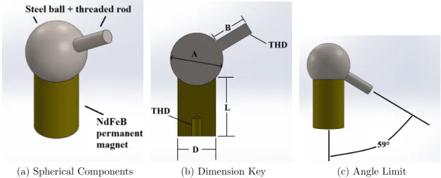
shows a range of common values for these magnets. The terminology in the table corresponds to the labels in Figure 2.3b, and all dimensions are in millimeters.

Table 2.1: Magnetic Spherical Joint Product Options [1]

Type D L A B THD Holding Force Cost

KD310 10 20 10 12 M3 18 N $3.65

KD312 10 20 12 12 M3 18 N $3.95

KD413 13 20 13 12 M4 40 N $4.84

KD418 13 20 18 12 M4 40 N $5.11

KD625 20 25 25 16 M5 150 N $6.55

KD725 25 35 25 16 M5 200 N $8.85

Cost, size, and holding force were all considered when selecting the magnetic spher-ical joints. In general, all three of these characteristics increase together. A lower cost spherical joint is preferred, especially since 12 joints are needed. This must be balanced by the need for sufficient holding force. If the holding force is too low, then the magnetic joint may separate during normal operation which must be avoided. The holding force cannot be too high either; if a binding condition occurs, the joint needs to be able to fail and separate. This prevents the linear actuator from stalling and overheating while relieving the acrylic plate loadings. The maximum force the linear actuators can exert is 35 lb, equivalent to 156 N. The KD625 seems to perfectly meet this requirement but there is very little cushion between the holding force and actuator force. On the other end, the KD310 is the lowest cost joint, but is dwarfed by the linear actuators, and can hold little more than the weight of the linear actu-ators. The KD418 was chosen as a moderate cost, size, and holding force solution, and it has functioned as intended in operation of the Stewart Platform.

(a) Spherical Components (b) Dimension Key (c) Angle Limit Figure 2.3: Magnetic Spherical Joint Properties

This angle is well beyond the angles of the linear actuators relative to the base and removes the joints as a limiting factor of range of motion. Friction was a concern ini-tially because of a lack of lubrication between the steel and magnet surfaces. Friction was very apparent when the steel ball was rotated against the magnet by hand, and smooth rotation was difficult to achieve. However, the rotation was much smoother once the linear actuator was attached to the joint. This is because the linear actu-ator provides several inches of leverage, whereas twisting the sphere or pushing the threaded rod only gives about an inch of leverage. When installed on the Stewart Platform, the actuators easily overcome friction and rotate smoothly.

2.3 Platform Material

platform. Wood and acrylic have lower densities than aluminum, but aluminum is stiffer, allowing for plate thickness and weight reduction; no material has a significant advantage for weight. Wood is around 2.5 times cheaper than acrylic and several times cheaper than aluminum for the same raw material volume. Reducing the plate thickness for aluminum still results in a much higher relative cost. All materials are able to be manufactured at Cal Poly; wood and acrylic can be cut using a laser cut-ter, and the aluminum can be cut with a water jet. While wood can be aesthetic, acrylic and aluminum are best suited to the Stewart Platform’s more industrial and mechanical appearance.

Acrylic was chosen because it is the best overall fit due to its moderate weight, cost, and easy to laser-cut. The base and top plates are both 1/4 inch thick acrylic sheets and weigh 2.67 lb and 1.66 lb respectively. For reference, if made out of aluminum 6061-T6 of equivalent size, their weights would be 6.02 and 3.75 lb respectively. Laser cutting of the acrylic was straightforward and resulted in aesthetic Stewart Platform plates. Additionally, acrylic is transparent which is beneficial because the electronics under the base platform are visible, exposing students to the components that control and drive the system.

2.4 Shaft Couplers

compliance. Bram Vanderborght gives a helpful introduction to compliance, sum-marizing that a compliant member will allow deviations from its equilibrium when a force acts on it, whereas a stiff member will not, within the device limits [23].

The magnetic joints, linear actuators, and acrylic are considered stiff components. However, the acrylic is the least stiff of the three so if the robot encounters a binding position or an unintended loading condition, the acrylic plates will take the load, risking deformation and breakage. This should be avoided by placing a compliant member in series with the linear actuator. The compliant member must be in a compact and professional package, and removable if the Stewart Platform can be run without the compliant member.

Helical shaft couplings were chosen to be the compliant member because they sat-isfied the above requirements. Shown in Figure 2.4, they are primarily intended for torque transmission but offer the flexibility in axial and bending motions to provide the necessary compliance. The shaft couplings chosen are the WAC20-4mm-4mm Aluminum Alloy Couplings and the data sheet is located in Appendix B.

2.5 6-3 Configuration Geometry

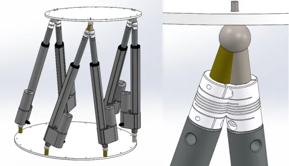
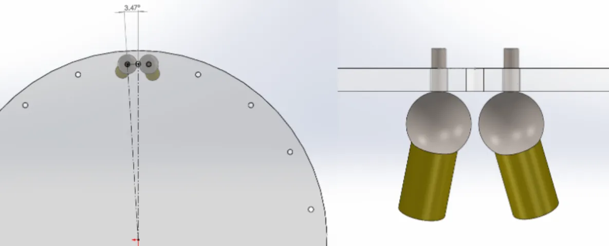
In a 6-3 configuration, the six base joints are evenly spaced at 60°angles and the three top joints are evenly spaced at 120°angles. Two actuators have to share a joint in this configuration. When two magnets are attached to a single steel ball to accomplish this, there is interference shown in Figure 2.5, where the Stewart Platform is in a normal position and orientation.

Figure 2.5: Range-of-Motion Limitation with Sharing Spherical Joint

Figure 2.6: Range-of-Motion Limitation with Sharing Spherical Joint

To fix this, the spherical joints had to be separated. Separation means the robot will not truly be in a 6-3 configuration, only close to it. The geometry of the spheres drove the angle separation of 3.47°between each joint from the 120° centerline is shown in Figure 2.7.

This solution creates a new problem; the joint angles for the 6-3 configuration are no longer at 120°because of this angle of separation. This joint angle must be included in the modeling and kinematic equations of the Stewart Platform. This implementation is discussed in Section 4.1.1.

2.6 Electronics Enclosure

There are a few key electronic components required for the operation of the Stewart Platform. These components include a power supply, microcontroller, motor driver, and connection ports, plugs, and switches. These components are further discussed and detailed in Chapter 3. The components must be housed in an electronics en-closure for safety and reliability, protecting users from contact with live power and internal components from careless or accidental handling. Optimally, the enclosure should be relatively lightweight and portable, provide sufficient airflow, and be easy to manufacture at a low material price. Furthermore, the enclosure is an appropriate means to connect the PA-14P motor and potentiometer through the included 6-pin connector.

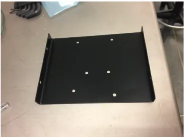
Sheet metal was chosen to be the electronics enclosure material because of its easy manufacturability, high strength, and low cost. Alternatives considered were plastic 3D printed enclosures or acrylic. The volume was too large and geometry too simple to justify all the 3D printed material. Acrylic could have been cut on the a laser cutter, but each surface would have to be fastened together. The sheet metal enclosure was designed, cut with a water jet, and bent using Cal Poly resources. The enclosure is shown in Figure 2.8

(a) Enclosure Front (b) Enclosure Rear Figure 2.8: Electronic Enclosure

that attach to the linear actuator connectors. On the walls of the enclosure are vents that allow air circulation. The enclosure will be attached underneath the base of the Stewart Platform, making the Stewart Platform and its electronics a complete unit.

The power supply resides in the bottom of the electronics enclosure. Suspended above it is the Arduino due and motor driver, to be discussed in Chapter 3, which helps keep the enclosure compact. This uninstalled bracket is shown in Figure 2.9. The drawings for all manufactured mechanical parts are located in Appendix C.

When the 6-pin female Molex connectors were inserted into the enclosure walls, the wall thickness was insufficient to retain the connectors. When the linear actuator was plugged in, the force would push the connector back into the enclosure, which would be impossible to bring back into place when the enclosure is installed under the Stewart Platform base. Retainers were printed to increase the wall thickness, allowing the connectors to stay in place when the linear actuators are plugged in. These retainers are shown in Figure 2.10. An additional benefit from these retainers is a permanent labeling solution, ensuring that the actuator number cannot be switched or removed.

Figure 2.10: Molex Connector Retainer and Label

Chapter 3

ELECTRONIC DESIGN

The electronic design of the Stewart Platform must meet the operational needs of the robot. The robot needs power to drive the actuators through its motions, which need to be accurately calculated and controlled. A controller can apply a control loop and send actuation signals based on calculated inputs and current positions of the linear actuators.

Figure 3.1: Stewart Platform System Diagram

drivers, and a power supply comprise the core electronic components. The bottom of the diagram incorporates the code inside the controller and the user interface with the Stewart Platform, discussed in Chapter 4.

3.1 Microcontroller - Brief Overview

A microcontroller uses a microprocessor, along with peripherals including read-only memory (ROM), random-access memory (RAM), and input and output capabilities (I/O) to make a computer on a chip [4]. They are typically used as part of an electronic or mechanical system with dedicated functionality. This is known as an embedded system, which are often subject to real-time constraints. There are count-less microcontrollers available to control the Stewart Platform.

3.1.1 Microcontroller Selection

a ready-made board, installing it, and downloading the project to the new board. This method is a near-turnkey solution to replacing the microcontroller.

Availability of usable software and resources was another driving factor in deciding to use the Arduino platform. This served to reduce development time, errors, and shift the development focus from setup to application and refinement. Progressive Automations has several examples of Arduino code that apply directly to their linear actuators. Examples of code applicable to this project include “Controlling Multiple Actuators with the Multimoto Arduino Shield” and “Controlling the Timing of a Single Linear Actuators Motion” [20]. The provided code helped with the setup and initialization required for working with the PA-14P actuators. Further details regarding the software used for operating the robot are discussed in Section 4.2.

(a) Isometric View (b) Top View Figure 3.2: Arduino Due [3]

3.1.2 Arduino Due Specifications

The following section describes the selected Arduino Due in further detail and its application to the Stewart platform. Table 3.1 summarizes some of the technical specifications of the Arduino Due.

Table 3.1: Arduino Due Technical Specifications [3]

Feature Value

Microcontroller AT91SAM3X8E Operating Voltage 3.3V

Digital I/O Pins 54 Analog Input Pins 12 Analog Output Pins 2

Flash Memory 512

SRAM 96 KB

Clock Speed 84 MHz

COM port to a connected computer. The Native USB connects to the SAM3X, en-abling serial communication over USB. The Native port can also emulate various USB devices, or act as a USB host. Both ports can be used for programming the Due, but there are some notable differences. When the Programming port is connected at 1200 baud and opened or closed, a SAM3X “hard-erase” procedure is performed, activating the Erase and Reset pins before UART communication. In comparison, the Native port performs a “soft-erase” procedure when opened and closed at 1200 baud. Flash memory is erased and the bootloader restarts the board. Programming via the Programming port is preferred because it is more reliable compared to the soft-erase procedure, which may not perform when the microcontroller has crashed. However, the Programming port is limited to a baud rate of 115200, which can be an issue if high-speed serial communication is required. The Native port is capable of much higher serial communication speeds because of the USB connection, and setting a baud rate in the Arduino sketch is ignored. This functionality and performance dif-ference was notable in programming and operating the robot. Uploading code using the Native port was several times faster than uploading via the Programming port. However, the Programming port was used when uploaded sketches crashed because of its reliability. For normal operations, functionality, and data transmission, the Native port was used [3]. All further information on the Arduino Due, including overview, technical specifications, and documentation, are available on the cited Arduino Due web page.

3.2 HexaMoto Shield

to complete the electronic hardware design. Two approaches include purchasing an aftermarket motor driver board or designing and assembling a custom board.

3.2.1 Design Requirements

The motor driver shield will need to have six channels to power each linear actuator. Each motor driver must provide a form of speed control. The robot operation would not be acceptable if the actuators could only operate at maximum speed. Addition-ally, it would be ideal to incorporate the potentiometer signals on the Arduino shield. This would provide an inclusive solution in which all inputs and outputs (except for 12V motor power) interface with the Arduino Due through the shield.

A potentiometer outputs a voltage as its analog signal. An 8-bit analog-to-digital converter (ADC) can output 256 discreet values. For a 4-inch stroke, each discreet change in the ADC reading of the potentiometer corresponds to a length of 0.0156 inches. For a 12-inch stroke, this value is 0.0469 inches. Similarly, a 10-bit ADC that outputs 1024 values means each increment is a change in length of 0.004 inches for a 4-inch stroke and 0.012 inches for a 12-inch stroke. It is important to note that ADCs have sources of measurement error, and they are not completely accurate to the above values.

Figure 3.3: Progressive Automation PA-14P Pinout [19]

3.2.2 Robot Power’s MultiMoto Arduino Shield

Progressive Automations has various products suggested for controlling and powering their linear actuators. One such product is a MultiMoto Arduino Shield, designed by Robot Power as shown in Figure 3.4.

(a) Isometric View (b) Top View

According to Robot Power’s website, the MultiMoto features four independently con-trolled and fully-reversible channels due to the use of the H-bridge design. Each channel can handle 6.5A continuous on a 6-36V input voltage. With current and over-temp limiting safety features, the general design and scope of the board is ap-propriate for the environment and application for the Stewart Platform. However, this board is two channels short of controlling the 6 linear actuators required on the Stewart Platform. It will however provide to be a useful reference point in designing a purpose-built driver. The schematics for the Robot Power Multimoto Arduino Shield are included in Appendix E.

3.2.3 HexaMoto Design

The HexaMoto is designed to meet all the requirements set in Section 3.2.1. It uses six L9958SBTR motor drivers, pin headers to interface with the Arduino Due, and 13 screw terminals for I/O. The specifics of these components are detailed in the following subsection. The schematic for the HexaMoto may be found in Appendix F.

Investigating different PCB vendors, JLCPCB offered two-layer boards under 100 mm by 100 mm at $2 for quantity five. This drove the overall dimension of the HexaMoto. By its own virtue, the shield must have pin headers that match with the Arduino due, so these were placed about the center plane. The motor drivers and their screw terminals were arranged around the bottom half of the board, and the potentiometer screw terminals were placed around the top half perimeter.

primarily routed vertically. This trace design helps keep traces organized and reduce overlapping and space issues, which are common occurrences when routing the last few traces of a board.

Figure 3.5: HexaMoto Board Layout, Top Layer

3.2.4 Component Details

3.2.4.1 STMicroelectronics L9958SBTR Motor Driver

The primary component of the HexaMoto Shield is the motor driver. The MultiMoto uses the L9958 motor driver [21] and it contains the functionality required for driving a Progressive Automation linear actuator. It is designed to drive brushed DC motors, and can output up to 8.6A at 4V to 28V. Protection features include undervoltage and overvoltage protection, and H-bridge over temperature and short circuits [22]. The block diagram and pinout of the selected PowerSO16 power package are shown in Figure 3.6.

Figure 3.6: L9958 Block Diagram and PowerSO16 Pinout [22]

Figure 3.7: L9958 Application Circuit [22]

All associated resistors and capacitors were included on the HexaMoto Shield. The 10nF capacitors on the outputs are decoupling capacitors, to reduce high frequency noise to the outputs. The 100µF and 1µF capacitors connected to Vs are for

decou-pling to increase the robustness of the output short protection.

An LED was used to visually indicate the direction of each L9958 motor driver’s output. The extension of the linear actuators is indicated by a green output. Retrac-tion of the linear actuators are indicated by a red output. This was accomplished by connecting the LED between OUTA and OUTB of the L9958 motor driver. This LED is made by SunLED, and shown in Figure 3.8.

3.2.4.2 I/O Hardware Components

Screw terminals were used for connecting the linear actuator wiring. 2-position screw terminals were used for the input voltage from the DC power supply unit, discussed in Section 3.4, and for the six outputs to the linear actuator motors. 3-position screw terminals, as shown in Figure 3.9b, connect the linear actuators’ potentiometer, comprised of the sensor, 3.3V, and GND. Pin headers are used to easily connect the HexaMoto Shield to the Arduino Due. Standard 0.10 inch pin headers are shown in Figure 3.9a. Note that the Arduino Due operates on +3.3VDC logic instead of +5VDC, hence the difference in the voltage used for the potentiometer.

(a) Pin Header, 0.10 in Pitch [7]

(b) Screw Terminal, 3 Position[8]

Figure 3.9: HexaMoto Shield I/O Hardware

3.3 HexaMoto Shield Assembly

and an oven. The stencil is a sheet of metal that is laser cut to match the solder pads on the PCB. The solder paste is applied to the stencil and distributed, resulting in a small and even deposit of solder paste on each pad. The components are placed on the PCB and then the PCB is put into an oven, allowing the solder to reflow. Figure 3.10 shows the HexaMoto Shield after reflow and cooling. Please note that solder paste can be irritating to the eyes, skin, and respiratory system. Make sure to handle solder paste with care, avoiding contact with eyes, skin, and vapor inhalation. Use isopropyl alcohol for solder paste cleanup.

Figure 3.10: HexaMoto Shield, Post Solder Paste Application and Reflow

Figure 3.11: HexaMoto Shield, Completed

After the assembly of the HexaMoto Shield was complete, it was fit-tested on the Arduino Due. The pin headers aligned and the shield fit on the Due successfully. During the fit test, it became apparent that the DI pin header was connected to the Arduino TX pin. The TX pin is the transmit pin for serial communication and while it theoretically can be used as a general purpose digital I/O pin, it is not realistic in practice. Therefore, the trace to the TX pin was broken and a jumper wire connected it to an available pin header.

3.4 DC Power Supply

Figure 3.12: PA-14P Current Draw vs Load [19]

A power supply unit was selected to support the maximum current draw of the system. If all linear actuators encountered a simultaneous maximum-load condition, then 30A would be drawn. A 12VDC, 360W power supply was chosen to supply the necessary power. With a maximum output of 30A, the unit can sufficiently power the robot. Additionally, the PSU has a built-in fan that always operates when powered. This provides intake towards the rear of the unit, and exhausts heated air through the front of the unit. Elevated temperatures were not noticed during extended cycle times. The electrical bill of materials may be found in Appendix G.

3.5 Connectors

The PC host connects to the Arduino with a B cable that plugs into the USB-B receptacle in the electronics enclosure. The receptacle is Digikey part number MUSB-D511-00 and is shown in Figure 3.13b.

(a) Power Receptacle (b) USB-B Receptacle

Figure 3.13: Power and USB Receptacle Connectors Enclosure

The Arduino Due requires a micro-USB connection. A micro-USB cable was spliced into the USB-B receptacle, as shown in Figure 3.14. This provides the intermediate connection between the host PC and the Arduino Due.

3.6 Electrical Assembly and Integration

The following details the progression of the electrical assembly and wiring of the electronic enclosure. First, the PSU, switch, and power receptacle were inserted and wired into the enclosure as shown in Figure 3.15.

Figure 3.15: Painted Electronic Enclosure with PSU and Connectors

(a) Beginning (b) Completion Figure 3.16: Enclosure Wiring

Chapter 4

SOFTWARE DESIGN

4.1 Matlab Platform Simulation

During the design stage, a kinematic simulation of the Stewart Platform was created using Matlab. This simulation uses the geometrical properties of the platform, and given a predetermined motion profile, calculates the joint lengths required to perform the move. Joint velocities are found by numerical differentiation of the joint lengths. Platform position, orientation, joint lengths and their respective velocities are plotted over time, with an accompanying 3D animation to visually verify the motion profile. Figure 4.1 shows the Stewart Platform oscillating by 15°about ψ, 2 inches above and below a Pz value of 20 inches, and increase linearly in θ from -15° to +15°.

Figure 4.1: Animation Screenshots

4.1.1 Geometrical Properties

connections. Similarly, the top vector is comprised of the distance and angle of the joint connections on the top plate. The top vectors must be rotated according to the orientation of the plate.

The simulation can be set for a true 6-6 configuration or 6-3 configuration. In a true 6-6 configuration, each joint on the base and top plate are spaced at 60°, which is set automatically in the simulation. In reality, this configuration is unstable, per the discussion in Section 1.3.1. Joints spaced other than 60° degrees apart will still be considered 6-6 configurations but the angles are set manually in the simulation setup. In the 6-3 configuration, there is an angle offset of the joints from the 120°centerline, as discussed in Section 2.5. This modifies Equation 1.3 to become

Bi=

        

B∗cos((i−1)∗60−angle)

B∗sin((i−1)∗60−angle)

0 1         

, Bi+1=

        

B∗cos((i−1)∗60+angle)

B∗sin((i−1)∗60+angle)

0 1          (4.1)

for i = 1, 3, and 5 where angle is 3.47° for this Stewart Platform.

4.1.2 Motion Profile

The motion profile in the simulation is predetermined and set independently for each degree of freedom. The duration of the motion is set in seconds. The number of steps within that duration can be set depending on how coarse or fine the simulation needs to be. Each of the six degrees of freedom can be set to a constant value, a continuous function, or a piecewise-defined function to achieve the desired motion. The motion profile used to create the animation in Figure 4.1 is included in Figure 4.2 as an example.

Figure 4.2: Motion Profile Creation

4.1.3 Calculation and Animation

The calculations for the joint lengths are completed in the Matlab simulation accord-ing to equations 1.11 and 1.12 in Section 1.3.3. In order to achieve the animation, the motion profile above (Figure 4.2) is linearly divided into hundreds of discreet steps over a specified time span. The inverse kinematics are calculated for each step giving a resolution equal to the motion profile time divided by the total number of steps. For example, the following plots show the length and velocities of linear actuators (Figure 4.3) for the given motion profile. This motion profile was specified to take 10 seconds and was calculated with 400 steps, for a resolution of 25 ms/step.

(a) Joint Lengths (b) Joint Velocitiess Figure 4.3: Matlab Simulation Plots for Joint Values

Figure 4.4: Matlab Simulation Plots for Orientation Values

Table 4.1 is provided as an example of these calculations for a Stewart Platform in a 6-6 configuration with the following values: a = 9 in, b = 7 in, θ = 0°, φ = −30°,

ψ = 45°, Px = 0, Py = 0, Pz = 22 in. A 3D representation of these values is shown in

Figure 4.5. These calculations are done for every step of the animation.

Table 4.1: Inverse Kinematics Solution for 6-6 Configuration

Loop 1 2 3 4 5 6

ax 9.00 4.50 -4.50 -9.00 -4.50 4.50

ay 0 7.79 7.79 0 -7.79 -7.79

az 0 0 0 0 0 0

bx 7.00 3.50 -3.50 -7.00 -3.50 3.50

by 0 6.06 6.06 0 -6.06 -6.06

bz 0 0 0 0 0 0

bx rotated 4.29 -2.14 -6.43 -4.29 2.14 6.43

by rotated 4.29 6.43 2.14 -4.29 -6.43 -2.14

bz rotated 3.50 1.75 -1.75 -3.50 -1.75 1.75

dx -4.71 -6.64 -1.93 4.71 6.64 1.93

dy 4.29 -1.36 -5.65 -4.29 1.36 5.65

dz 25.50 23.75 20.25 18.50 20.25 23.75

d 26.28 24.70 21.11 19.57 21.35 24.49

4.2 Arduino Sketch

The Arduino code must fulfill 3 primary requirements: Manage I/O, communicate over a serial connection, and run a control loop for the actuators. A state transition diagram, shown in Figure 4.6 was created to lay out the design of the code to achieve these design requirements.

First, the robot needs to establish serial communication with the host PC. Once this connection is made, then the robot will perform an initial calibration and homing procedure. Once successfully calibrated and homed, the code will wait for a com-manded position for each actuator. When received, the Arduino Due will run the control loop in the sketch and move the linear actuators.

Figure 4.6: Arduino State Transition Diagram

of the sketch, setup() runs once and after completion, loop() is repeatedly called. Custom functions can be declared in the sketch and called within loop().

4.2.1 Arduino Sketch Source Credit

The code satisfied the design requirement set above. Rather than developing brand-new code that would just result in near-identical function, the code was taken, with proper credit, verified, and adapted to this particular Stewart Platform, and may be found an Appendix J.

4.2.2 Setup and Initialization

The setup waits for the serial connection between the host PC and the NativeUSB port before starting. Once connected, the direction, PWM, and potentiometer pins are declared, and all outputs are set low. The control loop error is cleared to prevent premature or unexpected actuation. This setup is followed by a calibration and homing routine.

4.2.3 Calibration and Homing

4.3 Matlab GUI

A graphical user interface (GUI) was created using Matlab App Designer to allow users to easily connect to the robot and operate it. The user interface is shown in Figure 4.7, and the source code may be found in Appendix K. This section will cover the design choices and software flow of the app and its intended usage.

4.3.1 Serial Connection

Matlab first connects to the Arduino using serial communication over the COM port specified by the GUI. Determining the correct COM port is detailed in the Lab Man-ual. Once the correct COM port is entered, and the ’Calibrate’ button is clicked, the Stewart Platform begins its calibration procedure. When the calibration completes, the ’Calibrate’ button changes to ’Calibrated’. Only when the serial connection is successful and calibration is complete can the joint lengths be calculated. This portion of the GUI is shown in Figure 4.8.

Figure 4.8: Serial Connection and Calibration

4.3.2 Platform Configuration

the joints on the top plate. Both options allow the user to input the joint positions on the base plate. This portion of the GUI is shown in Figure 4.9.

Figure 4.9: Top and Bottom Joint Locations

4.3.3 Linear Actuator Position Calculation

The actuator lengths can now be calculated with the correct joint locations. The position and orientation of the platform is set by the user as desired. There are no software limits on the position and orientation values. There are dozens of possible configurations of the Stewart Platform, and each one has a different range of motion. Students will investigate the range of motion for two of these configurations. This portion of the GUI is shown in Figure 4.10.

Once the position and orientation of the Stewart Platform are given, the joint lengths can be calculated. It is important to note that if the joint positions are not set correctly, the length calculation will not be correct. At best, the robot will actuate to an incorrect position. Worse cases include the robot actuating to an unstable condition and collapsing. The results of the length calculation will be presented in two forms. The first form is in units of inches. If the length of any actuator is calculated to exceed its stroke to attain a certain position, an error will result. The robot will not be allowed to move to this location or be saved.

4.3.4 Saving and Sequencing Points

The user has the option to save the current calculated position under the ’Save and Sequence Setpoints’ panel shown in Figure 4.11. It can be saved in any of the six options. If a saved setpoint is no longer desired, it can be cleared, and saved setpoints can be overwritten. An option is provided to move to a setpoint after it has been saved.

4.3.5 Motion

This GUI panel, shown in Figure 4.12 contains the settings that alter the robot motion and the buttons that command robot motion. By checking the ’Enable Path Planning’ button, the controller will divide the move into smaller moves specified in the ’Points’ text box. This path is normalized in each degree of freedom via interpolation.

Figure 4.12: Motion Control Panel

Chapter 5

TESTING AND FUTURE WORK

5.1 Testing

Testing was performed on the linear actuators to ensure that they would achieve the length commanded. Table 5.1 contains the data taken for each actuator as they were commanded from 0 to 8 inches in 1 inch increments. The measurements were taken with a tape measure with a resolution of 1/16” (0.063”), and measured values interpolated to the nearest 1/32” (0.031”). The data shows that the actuators were accurate to within 1/16 of an inch across the entire stroke.

Table 5.1: Commanded and Actual Actuator Lengths

Input Actuator 1 Actuator 2 Actuator 3 Actuator 4 Actuator 5 Actuator 6

0 0.00 0.00 0.00 0.00 0.00 0.00

1 1.00 1.00 1.00 1.00 1.00 1.00

2 2.00 2.00 2.00 2.00 2.00 2.00

3 3.00 3.00 3.00 3.00 3.00 3.00

4 4.00 4.06 4.03 4.03 4.03 4.03

5 5.00 5.06 5.06 5.03 5.03 5.03

6 6.03 6.06 6.06 6.03 6.03 6.03

7 7.06 7.06 7.06 7.03 7.03 7.03

8 8.06 8.06 8.06 8.03 8.03 8.03

The position of the Stewart Platform was measured first. The height (Z) was simply measured from the top surface of the base platform to the top surface of the moving platform. This measurement was taken with a tape measure with markings every 1/16 inches. The moving platform position in the x-axis and y-axis was measured by attaching a weighted pendulum to the top platform, which would make contact with a ruled grid placed on the base platform below. The grid had markings every tenth of an inch. Table 5.2 contains the nominal values input to the GUI and the actual position achieved by the Stewart Platform.

Table 5.2: Stewart Platform Positional Test Measurements

X [in] Y [in] Z [in]

Input Measured Input Measured Input Measured

-4 -4.25 -4 -4.20 18 17.94

-3 -3.20 -3 -3.10 19 18.97

-2 -2.10 -2 -2.05 20 20.00

-1 -1.05 -1 -1.00 21 21.00

0 0.00 0 0.00 22 22.00

1 1.05 1 1.00 23 23.00

2 2.10 2 2.00 24 24.03

3 3.15 3 3.10

4 4.20 4 4.20

The platform was most accurate at the center of its positional range of motion. The height of the platform was very accurate and had a maximum error of 1/16” at the minimum height and 1/32” at the maximum height. The error along the x-axis and y-axis increased fairly linearly, by approximately 0.05 inches per inch.

the y-axis; each axis was measured separately. The measurement resolution of the inclinometer was 1°. Examples of these measurements are shown in Figure 5.1.

Figure 5.1: Inclinometer App Example Readings

Table 5.3: Stewart Platform Orientation Test Measurements

θ [degrees] φ [degrees] ψ [degrees]

Input Measured Input Measured Input Measured

-30 -30 -30 -31 -60 -61

-25 -24 -25 -26 -50 -51

-20 -19 -20 -20 -40 -41

-15 -14 -15 -15 -30 -30

-10 -9 -10 -10 -20 -20

5 -4 -5 -5 -10 -10

0 0 0 0 0 0

5 4 5 4 10 10

10 10 10 9 20 19

15 15 15 14

20 20 20 19

25 25 25 24

30 30 30 29

5.2 Conclusion

A Stewart Platform was successfully designed, assembled, and implemented as part of a lab experiment. It covers many facets of robots at an introductory level, in-cluding inverse kinematics, simulation, assembly and disassembly, and motion imple-mentation. Using the platform does not require a steep learning curve and performs satisfactorily for student experimentation. The mechanical design allows for easy re-configuration and uses the magnetic joints as the mode of failure, protecting the rest of the system components. While the Stewart Platform is an overall success, it is open to further improvements and future work.

5.3 Improvements

5.3.1 HexaMoto Shield

Figure 5.2: HexaMoto Shield Improvements

The placement of screw terminals could also be changed to improve ease of assembly. The labels 1-6 correspond to the linear actuator. The potentiometer and power terminals are separated across the board. Pairing these terminals by mirroring across the horizontal would make more sense, as only actuators 3 and 4 would be separated across the board. During board design, pairing the power and potentiometer terminals was attempted, but it was ultimately decided to keep the motor drivers together.

5.3.2 Acrylic Plates

Platform is reconfigured per the lab manual. Aluminum threads can wear down under these conditions.

The current angle spacing on the base and moving platforms is 20°. A spacing of 30° may be more appropriate; 20°spacing offered a few too many configuration options, and 30° spacing is more intuitive when using sine, cosine, and the x and y-axes. Additionally, the angles increased in the clockwise direction from a top view. This should be changed to counter-clockwise in order to follow the right-hand rule for Cartesian coordinates. Currently, CW results in +Z in the downwards direction.

To achieve this, the material would have to be sourced and purchased. If using only Cal Poly resources is desired then the aluminum should be cut with a water jet. Once cut, the threads in the top platform would need to be tapped, ideally for threaded inserts.

5.4 Future Work

A method of jogging the robot would be a helpful addition to the Stewart Platform. This could be accomplished using buttons mapped to increasing or decreasing the value of a degree of freedom. A joystick, a phone, or a 3D mouse (Figure 5.3) would be particularly suited to controlling a Stewart Platform.

This device is able to sense in all 6 degrees of freedom, which matches the Stewart Platform. Any user input to the 3D mouse would be matched by the moving platform. The mouse can also sense magnitude. A light push or twist of the mouse could jog the robot slowly, and larger twists etc. would result in faster jogging.

Figure 5.3: 3Dconnexion 3D Mouse [2]

Chapter 6

LAB MANUAL

6.1 Lab Manual

A lab manual was developed in conjunction with the Stewart Platform. The experi-ment investigates inverse kinematics, reconfiguration, range-of-motion, and use of the Stewart Platform as a flight simulator. The simulation script from Section 4.1 will be used by students to verify their inverse kinematics. Next, the students will reassemble the robot into two configurations, and determine the range-of-motion of each. Finally, students will plan and run a movement sequence to simulate basic flight motion. The full lab manual can be found in Appendix L.

6.2 Learning Objectives

BIBLIOGRAPHY

[1] AliExpress. KD418 Universal ball and socket joint, 2019. Accessed 8 October 2019.

[2] AmericanXplorer13. Space navigator. Web, March 2007. Accessed 5 February 2020.

[3] Arduino. ARDUINO DUE, 2019. Accessed 22 June 2019.

[4] K. J. Ayala. The 8051 microcontroller. Cengage Learning, 2004.

[5] P. Cruz, R. Ferreira, and J. Silva Sequeira. Kinematic modeling of stewart-gough platforms. ICINCO, 2005.

[6] B. Dasgupta and T. Mruthyunjaya. The stewart platform manipulator: a review. Mechanism and Machine Theory, 35(1):15–40, December 1998.

[7] Digi-Key. Molex 0022284060. Web, August 2019. Accessed 18 August 2019.

[8] Digi-Key. Molex 0398800303. Web, August 2019. Accessed 18 August 2019. [9] Digi-Key. SunLED XZMDKVG55W-4. Web, August 2019. Accessed 18

August 2019.

[10] Firgelli Automations Team. Linear Actuators 101 - Everything you need to know about Linear Actuators. Web, November 2018. Accessed 13 June 2019.

[11] IBS Magnet. Magnetic ball joints, 2019. Accessed 13 June 2019.

[13] Matthewbarry. Eric gough’s tire testing machine. Web, March 2016. Accessed 10 January 2020.

[14] McMaster-Carr. Ball Joint Rod Ends Datasheet, 2019. Accessed 13 June 2019.

[15] J. Merlet. Parallel Robots. Springer Netherlands, P.O. Box 17, 3300 AA Dordrecht, The Netherlands, 2006.

[16] S. B. Niku. Introduction to Robotics: Analysis, Control, Applications. John Wiley and Sons, 2nd edition, 2011.

[17] S. B. Niku. Introduction to Robotics: Analysis, Control, Applications. John Wiley and Sons, 3rd edition, 2020.

[18] Progressive Automations. Multimoto arduino shield. Web, August 2019. Accessed 18 August 2019.

[19] Progressive Automations. PA-14P Datasheet, 2019. Accessed 13 June 2019.

[20] Progressive Automations. Resources. Web, August 2019. Accessed 19 August 2019.

[21] Robot Power. Multimoto product information. Web, August 2019. Accessed 18 August 2019.

[22] STMicroelectronics. L9958, December 2013. Accessed 20 August 2019.

[23] B. Vanderborght. Compliant robots. Web, January 2012. Accessed 10 October 2019.

APPENDICES

Appendix A

PA-14P DATASHEET

Contents

PA-14P

Data Sheet

2 3 4 5 6 7 8 Specifications

Dimensions

Speed/Current vs Load

Specifications

2

1" to 40"

Internal - Non-Adjustable Customizable

ACME Screw

Brushed or Brushless DC Motor See Page 5

40" (customizable) 6062 Aluminum Alloy

Aluminum Alloy/Stainless Steel (customizable)

Polyformaldehyde (35 lbs only)/Powder Metallurgy Steel Alloy Silver

Silver <45dB

25% (5 minutes on, 15 minutes off)

-25ºC to 65ºC (-13ºF to 149ºF) IP54 (IP65 customizable) Potentiometer (see page 5) CE/RoHS

See Page 6

Customizable Stroke

Limit Switch

Limit Switch Feedback Screw Type Motor Type Connector Type Wire Length Housing Material Rod Material Gear Material Color (Shaft) Color (Motor End) Noise Duty Cycle Operational Temperature Protection Class Feedback Options Certifications Mounting Brackets Mounting Ends Full Load

Load (LBS) Speed (inch/sec)

No Load No Load Current (A)

12VDC 24VDC 36VDC 48VDC

0.3 0.3

Full Load Current (A) 12VDC 24VDC 36VDC 48VDC

PA-14P Stroke 6.511 7.51 8.513 9.514 11.51 13.51 14.51 15.51 17.51 19.51 21.51 23.519 12 16 7.51 9.51 11.51 13.51 17.51 21.51 23.51 25.51 29.51 33.51 37.51 41.51

Dimensions

Hole to Hole

2 6 8 20

25.51 27.51 45.51 49.51 24 29.51 35.51 53.51 66.61 A B 40 45.51 85.51

10 14 18 22 30

For Stroke Length

A = Stroke Length + 5.51" B = Stroke Length x 2 + 5.51"

3

Speed vs Load

Current vs Load

Connectors & Feedback

5

1

2

2-Pin Connector (Standard)

Component Part Number

Housing 39-01-2025

Part Name

Molex Mini Fit Jr 2-Pin Receptacle

Mating Part Number

39-01-3029/ 39-01-2026

Resistance* 0-10kΩ

Tolerance +/- 5% Number of Turns

10

Potentiometer Specifications

Signal

+5VDC gnd

*Actual resistance value may vary within the 0-10kΩ range based on stroke length *For Stroke Length up to 40"

1 2

M- M+

Mounting Brackets

6

BRK-14

Ø0.07 0.99 0.76

0.14

0.18

Ø0.23

Ø0.38

Ø0.23 Ø0.10

1.26 1.34 1.15

1.04 0.12

1.74 1.74

2.30 0.68

0.32

1.43 R0.32

0.36 1.04

0.57

R0.18

2.30 Ø0.32

0.52

0.49

(Dimensions in inches)

BRK-03

M4 x 16 Bolt

M4 Hex Nut

Internal Components