INFORMATION THEORETIC INTERPRETATIONS OF RENORMALIZATION GROUP FLOW
Raymond Eveleth Fowler III
A dissertation submitted to the faculty of the University of North Carolina at Chapel Hill in partial fulfillment of the requirements for the degree of Doctor of Philosophy in the
Department of Physics.
Chapel Hill 2019
©2019
ABSTRACT
Raymond Eveleth Fowler III: Information Theoretic Interpretations of Renormalization Group Flow (Under the direction Louise Dolan and Jonathan Heckman)
We interpret the renormalization group flow between quantum field theories as a communication channel problem, which allows us to quantify UV-IR mixing in terms of information theoretic quantities, i.e., we can quantify the information of the UV theory that remains accessible in the IR theory. Because of the AdS-CFT interpretation of the renormalization group flow, our interpretation applies to the AdS-CFT correspondence too.
In our interpretation, the UV variables are the input signal for the channel, the output variables are the IR variables resulting from the renormalization group flow, and the renormalization group transformation is viewed as the communication channel. To make this interpretation, we make use of the Kullback-Leibler (KL) divergence, which quantifies the information theoretic distance between two probability distributions. In order to use the KL divergence with quantum field theories, we study the probability distributions associated with Euclidean quantum field theories; the KL divergence thus computes the relative entropy between these Euclidean quantum field theories, as in statistical field theory. We then use the renormalization group and the techniques of effective field theory to find the probability distributions that we need to use with the KL divergence in order to measure the information lost upon performing the renormalization group transformation.
TABLE OF CONTENTS
LIST OF FIGURES . . . viii
LIST OF ABBREVIATIONS . . . xi
1 Introduction . . . 1
2 Effective Field Theories in the Standard Model and Beyond . . . 7
2.1 Standard Model–Overview . . . 9
2.2 Excursis: Hierarchy Problem . . . 14
2.3 Supersymmetry . . . 16
2.4 String Compactification . . . 18
2.5 Excursis: Kaluza-Klein Compactification . . . 20
2.6 Intersecting Branes and Chiral Matter from M/F theory . . . 21
2.7 Excursis: Warped Large Extra Dimensions . . . 25
3 Renormalization Group–Overview . . . 28
3.1 Kadanoff . . . 28
3.2 Wilson . . . 31
3.3 Wilson and the Callan-Symanzik Equation . . . 33
3.4 Polchinski . . . 34
3.5 AdS/CFT Holography . . . 36
3.6 RG in General . . . 37
4 Communication Channel . . . 39
4.1 The KL Divergence . . . 39
4.2 Channel Capacity and UV/IR Mixing . . . 44
4.4 Information Bottleneck . . . 48
4.5 Quantum Relative Entropy . . . 51
5 Decimation . . . 53
5.1 Different Decimation Procedures . . . 58
5.2 Thermodynamic Interpretation . . . 59
6 Continuum . . . 61
6.1 CFTs . . . 61
6.2 Continuum RG Result . . . 62
6.3 Fast and Slow Modes . . . 65
6.4 Matching Lattice to Continuum: Part 1 . . . 68
6.5 Matching Lattice to Continuum: Part 2 . . . 71
7 Warm-up Example: Ising Model Perturbations . . . 74
7.1 1D Perturbations . . . 76
8 Example: Ising Model Decimation. . . 84
8.1 1D Decimation . . . 84
8.1.1 1D Decimation: Rescaling . . . 91
8.2 2D Decimation . . . 94
8.2.1 2D Decimation: Rescaling . . . 106
8.2.2 2D Decimation: Mean Field Theory . . . 110
8.3 (1 + epsilon) Dimensions . . . 112
9 Channel Capacity Example: Ising Model . . . 116
9.1 1D Ising Model on Tree . . . 116
10 Continuum Examples . . . 122
10.1 Scalar field . . . 122
10.2 Irrelevant deformation . . . 123
11 Conclusion . . . 127
APPENDIX A: MATHEMATICA CODE FOR 1D ISING MODEL FIGURES . . . 130
APPENDIX B: MATHEMATICA CODE FOR 2D ISING MODEL FIGURES . . . 137
LIST OF FIGURES
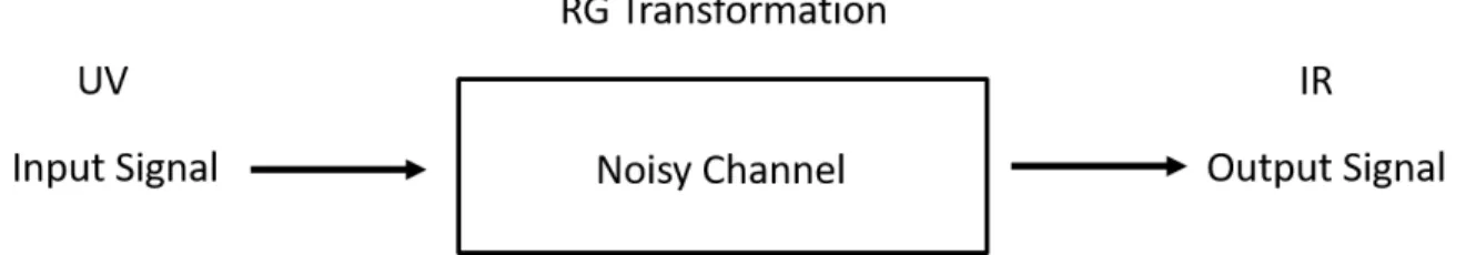
1.1 A schematic representation of viewing the RG transformation as a noisy com-munication channel. The variables of the UV theory are the input. The RG transformation is the noisy channel that produces the output variables of the
IR theory. . . 2 1.2 A schematic representation of viewing the RG transformation as
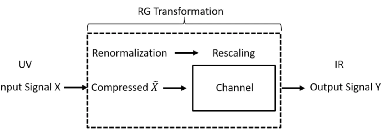
communica-tion through an informacommunica-tion bottleneck. The variables of the UV theory are the input. The renormalization/coarse-graining step of the RG transformation performs the compression toX˜. The re-scaling step sends the compressed
variables to the output IR theory. . . 3
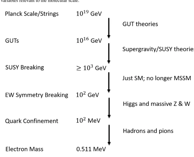
2.1 A representation of effective theories of particle physics. We start with the Planck scale and go all the way down to the scale of the electron mass. At each scale, a new effective theory with its own fields becomes the useful description,
especially as symmetries are broken with the lowering of the energy scale. . . 8
3.1 An example of grouping spins into blocks in a 2D lattice. In this particular case of blocking, the blocks are squares and contain nine spins; the center spin is chosen for the block, resulting in a lattice with fewer spins and a greater spacing between spins. Other blocking methods could be chosen, e.g., triangles,
and different amounts of spins could be included in the blocks. . . 29
5.1 A 2D lattice of with sites labeled as black and white as a preparation to
decimating the lattice. . . 53 5.2 A 2D lattice of white sites after decimating the black sites. The lattice is rotated
by 45 degrees relative to its original orientation, as can be seen by simply rotating it by 45 degrees, and the nearest neighbors lie along the diagonals of the squares of the original lattice, resulting in a lattice spacing of√2times the
original lattice spacing. . . 54 5.3 A 1D chain of sites labeled as black and white as preparation for decimating
the lattice. The lines show which sites are coupled to each other (nearest neighbors). . . 59 5.4 Result of decimation of white sites of 1D lattice before rescaling. Rescaling
just changes the spacing between the sites to the original lattice spacing. . . 59 5.5 Result of decimating white sites of 1D lattice, then black sites, and forming a
joint distribution. . . 59
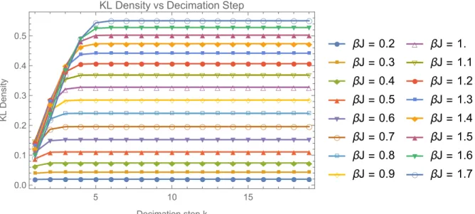
8.1 The KL density for the 1D Ising model as a function of decimation step for fixed, low values ofβJ. There is no critical value for the 1D Ising model, but
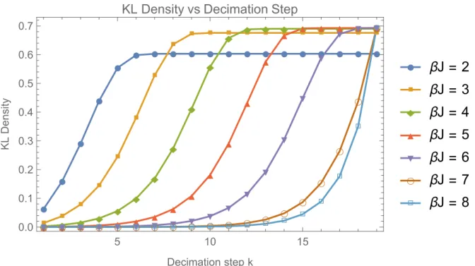
8.2 The KL density for the 1D Ising model as a function of decimation step for fixed, higher values ofβJ. We start to see the curves converge on the final
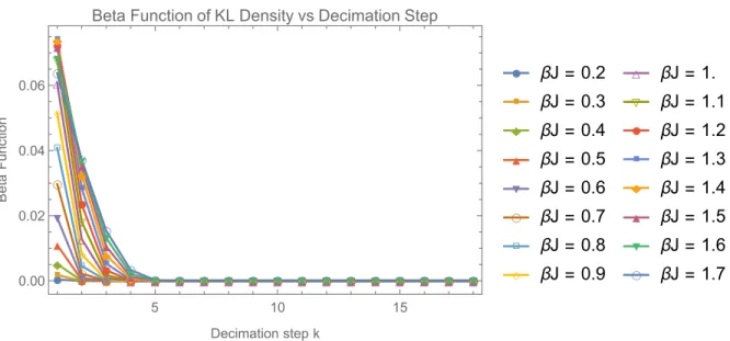
curve shown in this figure. . . 87 8.3 The beta function of the KL density for the 1D Ising model as a function of
decimation step for fixed, low values ofβJ. These are the same values that
were used for the KL density at low values ofβJ. . . 89 8.4 The beta function of the KL density for the 1D Ising model as a function of
decimation step for fixed, higher values ofβJ. These are the same values that
were used for the KL density at higher values ofβJ. . . 90 8.5 The KL density for the 1D Ising model as a function of decimation step for
fixed, low values ofβJ. The distributionq is formed from decimation plus rescaling. There is no critical value for the 1D Ising model, but we cover the
parameter space that includes the critical value of the 2D Ising model. . . 92 8.6 The KL density for the 1D Ising model as a function of decimation step for
fixed, high values ofβJ. The distributionqis formed from decimation plus
rescaling. We start to see the curves converge on the final curve shown in this figure. . . 93 8.7 The KL density for the 2D Ising model as a function of decimation step for
fixed values ofβJabove the critical value≈0.50698. . . 96 8.8 The KL density for the 2D Ising model as a function of decimation step for
fixed values ofβJbelow the critical value≈0.50698. . . 97 8.9 The beta function of the KL density for the 2D Ising model as a function of
decimation step for fixed values ofβJ above the critical value≈0.50698. . . 98 8.10 The beta function of the KL density for the 2D Ising model as a function of
decimation step for fixed values ofβJ below the critical value≈0.50698. . . 99 8.11 The KL density for the 2D Ising model as a function of the couplingβJ for
various decimation steps. Only a few steps are shown because the curves merge to the exact same curve around decimation step 8, i.e., the KL density stops significantly changing after each decimation step after around eight decimation
steps. The critical value is≈0.50698. . . 101 8.12 The KL density for the 2D Ising model as a function of the couplingβJ after
one decimation step. The critical value is≈0.50698. . . 102 8.13 The KL density for the 2D Ising model as a function of decimation step for
fixed values ofβJ below the critical value of≈0.50698. The distributionq
is formed from decimation plus rescaling. There are similarities to the results when using decimation plus forming a joint distribution for values below the
8.14 The KL density for the 2D Ising model as a function of decimation step for fixed values ofβJabove the critical value of≈0.50698. The distributionqis formed from decimation plus rescaling. These are very different results from when using decimation plus forming a joint distribution: notably, the curves
LIST OF ABBREVIATIONS
ADE An object that corresponds to the A, D, or E type of simply laced Dynkin diagrams AdS Anti-de Sitter space
CFT Conformal Field Theory EFT Effective Field Theory
EW Electroweak
h.c. Hermitian Conjugate GUT Grand Unified Theory
IR Infrared
KL Kullback-Leibler
KK Kaluza-Klein
LED Large Extra Dimension
MERA Multi-scale Entanglement Renormalization Ansatz MSSM Minimally Supersymmetric Standard Model RG Renormalization Group
SM Standard Model
SUGRA Supergravity SUSY Supersymmetry
QED Quantum Electrodynamics QCD Quantum Chromodynamics QFT Quantum Field Theory
UNC University of North Carolina at Chapel Hill
CHAPTER 1 Introduction
Effective field theories provide a general framework for organizing and calculating physical phe-nomena. Different particles and physical phenomena become relevant for calculations and observation at different energy and distance scales. Accordingly, there are different effective field theories for the different scales at which physics occurs: the effective field theory at each scale allows for making calculations taking into consideration only those phenomena that are relevant to the scale of the problem, simplifying calculations. The effects of the particles and physics at higher energy and smaller distance scales (called ultraviolet physics) are incorprated into the coupling constants of the lower energy (called infrared physics) effective field theory, and when an effective field theory has divergences or broken symmetries, changing the scale of the theory to higher energies where new particles become relevant to interactions can remove or soften the divergences and restore the symmetries. An effective field theory that breaks down at some energy scale is then not a problem of the theory but a feature: it just means the effective theory is not the full theory, not containing all particles and their interactions. In the effective field theory framework, all theories in physics are effective theories, except for the fundamental theory at the highest of energy and smallest of distance scales.
A renormalization group (RG) flow is used to change the scale of a theory and generate effective field theories. In performing a renormalization group flow down from ultraviolet (UV) scales to IR scales, mixing between the UV and IR modes (UV-IR mixing) will occur. This gives rise to the possibility of detecting UV effects–and in particular, string compactification effects–while being able to only access the IR physics of the effective field theory.
Therefore, some questions arise: Is there a way to quantify this UV-IR mixing in order to distinguish between similar IR theories and thereby access information about the UV, and if so, how can this be done? It could also turn out that the measure used to distinguish the UV theories will show that classes of UV theories are indistinguishable: applying this to string theory means that classes of string theories could turn out to be indistinguishable according to this measure, thereby reducing the number of distinct string vacua.
Figure 1.1: A schematic representation of viewing the RG transformation as a noisy communication channel. The variables of the UV theory are the input. The RG transformation is the noisy channel that produces the output variables of the IR theory.
Our answer is that we can think of the UV information accessible at the IR physics as a signal sent from the UV scale to the IR scale. The renormalization group transformation is then viewed as a noisy communication channel that the UV information traverses to the IR scale. We can thus evaluate the mutual information and find the channel capacity of the channel. See Figure1.1for a schematic representation of this idea.
before rescaling the lattice or momentum). See Figure1.2for a schematic representation of this idea. We explore this idea a little in this thesis to show how the bottleneck concept works in general and would work with our ideas, but we do not fully develop this point, and we ultimately conclude it is easier to just calculate the KL divergence and interpret our results in terms of Figure1.1.
Figure 1.2: A schematic representation of viewing the RG transformation as communication through an information bottleneck. The variables of the UV theory are the input. The renormalization/coarse-graining step of the RG transformation performs the compression toX˜. The re-scaling step sends the compressed variables to the output IR theory.
In short, we can think of the renormalization group flow in terms of information theoretic quantities and thereby provide a direct, information theoretic measure of the UV information accessible at the IR scale. The renormalization group flow can also be thought of in terms of the AdS/CFT correspondence, where the energy scale associated with renormalization goes in the direction of the bulk AdS space as in, e.g., [4–7], so we are also providing an information theoretic interpretation of the AdS/CFT view of the renormalization group flow.
Thinking along these terms, we will make use of the Kullback-Leibler (KL) divergence as in [8,9] to measure the information difference. For normalized probability distributionspandq, it is,
D(p||q) = Z
Dµ plogp
q, (1.1)
While progress has been made in calculating the UV information in the IR physics by using the geo-metric entanglement entropy [10–14], using the KL divergence has some advantages over the geogeo-metric entanglement entropy [15,16]. The geometric entanglement entropy depends on the geometry of how the subspaces of the Hilbert space are formed: the KL divergence does not depend on the geometry. The geometric entanglement entropy also has difficulties being defined for gauge theories and dealing with extended objects like Wilson loops [17], while there is a possibility of using the KL divergence with gauge theories since all one needs is a well-defined probability distribution produced by the gauge theory’s action. Furthermore, the interpretation of the renormalization group flow as a communication channel, thereby allowing for interpretation of the whole problem in information theoretic terms, has not yet been considered in uses of the geometric entanglement entropy.
There are other measures of information loss under the RG flow via the A and C theorems. In 2D, there is a numberCthat decreases monotonically under the RG flow and is equal to the central charge at fixed points of the RG flow [18]. Similarly, for other even dimensions, there is a numberA[19–21]. For odd dimensions, sphere partition functions provide this monotonically decreasing quantity [22,23]. Because these numbers decrease monotonically under the RG flow, they provide some measure of the degrees of freedom that are lost under the RG flow and thereby some measure of the information loss. However, there are two difficulties with using these quantities to quantify information loss. The first is that these theorems are only proven in 2D, 3D, and 4D: the rest is yet to be proven still. The second is that these numbers do not directly quantify the information loss: the numbers decrease with information loss, but unlike the KL divergence, they do not directly measure the information loss in terms of, e.g., bits.
We will proceed as follows. We first discuss effective field theories in Section2. In that section, we show many examples of effective field theories, their problems, and how new UV physics continues to fix effective field theories as the scale goes to higher and higher energies. We start with the Standard Model, then discuss grand unified theories and supersymmetry, then finally string theory compactifications. At the end of the section, we discuss warped large extra dimensions, since it ties in nicely with an AdS/CFT interpretation of the renormalization group flow.
the connection between the RG flow and AdS/CFT in Section3.5and close the section by discussing the RG procedure in general to prepare for discussing the information theoretic connection.
Next, in Section4we discuss the concept of a communication channel and the tools used for making calculations of quantities related to a communication channel. We first discuss the KL divergence in Section4.1and then subsequently discuss its use in calculating information-theoretic quantities, such as the mutual information and the channel capacity. After discussing the channel capacity, we make the connection to an information theoretic interpretation of the RG flow in Section4.3. We then discuss the information bottleneck as another possible information theoretic quantity of interest to our problem and finish the section by discussing how our procedure with the KL divergence connects to the quantum theory.
In the discussion of the communication channel and the KL divergence, it is noted in the beginning of Section4.2that a difficulty in using the KL divergence to measure UV-IR mixing is that it naively requires the use of marginalizing distributions over IR modes, i.e., integrating out IR modes. Integrating out IR modes leads to non-local interactions in the effective field theory. Another difficulty that is noted in Section4.1is that the KL divergence is quadratic to leading order, which leads to integrated two-point functions and contact terms.
We therefore study these difficulties next and work to find a way around them. We do so by studying lattice theories first and then continuum theories. We consider lattice theories in Section5, studying a particular RG procedure for general lattice field theories: the decimation procedure. The lattice theories are in position space and so do not have the conceptual difficulty of integrating out IR modes, and the lattice theories come with a natural regulator (the lattice spacing), so there is no need for concern about contact terms. We find that there are two different ways to perform the decimation procedure so as to calculate the mutual information between a UV theory and an IR theory resulting from the decimation procedure. At the end of the section, we show an interpretation of the mutual information in terms of thermodynamic quantities.
lattice theories and find that both decimation procedures produce the same result in the continuum limit. Finally, in Section6.3, we find a way to define a UV completion for continuum theories when using the KL divergence with continuum theories. The UV completion removes the contact terms of our earlier result. We then find the energy scale dependence of the information of the UV theory in the IR theory.
Having discussed and done much theoretical formulation and general calculations, we then make concrete calculations for a variety of example models, starting with lattice models and then continuum models. As a warmup example, we first find the KL divergence between an Ising model and an Ising model with a perturbation in Section7. We consider the general calculation for both 1D and 2D Ising models and then we make a specific calculation with the 1D model, where we also find the thermodynamic largeN limit for the 1D model. We then make calculations for example decimated theories in Section8. We study both 1D and 2D Ising models, along with a(1 +ε)D model. We make progress towards an example calculation of the channel capacity in Section9by studying a 1D Ising model on a tree, which also provides an example of a more general block renormalization group procedure.
CHAPTER 2
Effective Field Theories in the Standard Model and Beyond
The idea of low energy physics being sensitive to the physics at higher energies is encapsulated in the framework and machinery of effective quantum field theories. Start with a quantum field theory defined by an actionSΛwith a cutoffΛ. An effective quantum field theory is produced by integrating out higher energy modes down to some lower energy scaleΛ0to produce an actionSΛ0 [24]. The mathematics of this will be discussed in more detail with the discussion of the Renormalization Group in Section3. See also [25] for another mathematical treatment of effective field theories.
The effective field theory is understood as capturing the physics that exists at the energy scaleΛ0, which provides a regulator for the theory [24]. The end result of the process of convertingSΛtoSΛ0 is that higher energy variables are eliminated (they are integrated out), which then allows for describing the theory in terms of variables that exist at the lower energy scale. The effects of the higher energy variables are encoded in the coupling constants of the lower energy variables.
Thinking of effective actions in terms of Feynman graphs, consider a diagram at the original scaleΛ that includes interactions of the higher energy particles with the lower energy particles. The effective action at scaleΛ0will have intersecting lines in place of the loops and exchanges of the higher energy particles. Reversing the process by changing the scale back to the originalΛresults in replacing the point where the lines intersect with loops and exchanges of the higher energy particles [25].
This Feynman graph picture of effective field theories helps conceptualize what an effective action is describing in terms of particles. There are high energy particles that cannot be detected (or have highly suppressed interactions) at lower energies. Thus, the exchange and interactions of these higher energy particles cannot be detected when computing the interactions of the lower energy particles. Instead, there is an effective interaction of the lower energy particles that remains.
collective effect at each energy scale. Taking this perspective of effective field theories, we see that all non-fundamental descriptions of physics are effective theories, and therefore, all physics is dependent on the energy scale of the problem. Furthermore, because physics can be described in terms of quantities that are detectable at a particular energy scale, one does not need the full, fundamental description of physics in order to make use of physics at a lower energy scale.
The dependence of physics on energy scale is in fact the usual procedure in physics. For the purposes of describing books sliding on ramps, one uses books, centers of mass, normal forces, and friction; one does not describe the purpose in terms of the molecular interactions that make up the friction, normal force, books, and ramps. However, if one wished to describe molecular interactions, one must use variables relevant to the molecular scale.
As an example of an effective quantum field theory, consider the strong interaction [26,27]. At a high energy scale (the QCD scale), we can describe our theory in terms of quarks and exchanges of gluons. For lower energies, spontaneous chiral symmetry breaking occurs, producing Goldstone modes. In this case, the Goldstone modes are pions. If we are not at a high enough energy scale where we need to describe physical objects and interactions in terms of quarks and gluons, the pion Lagrangian is easier to use for describing the lower energy effective interactions, thereby showing the utility of effective field theories. See Figure2.1for a graphical diagram of effective field theories as the energy scale is lowered; we will discuss a number of these effective theories in the sections that follow.
Effective field theories are not only useful for calculations, but they are also useful for removing UV divergences in a theory and for naturally having new particles at higher energies than the scale of a particular effective theory. Furthermore, because effective field theories encode the UV physics in the coupling constants of the lower energy theory, effective field theories provide a useful way to think about the problem of quantifying information about UV physics that is present in the IR physics. Furthermore, in the cases where a variety of different theories at a UV scale produce similar effective field theories at the IR scale, quantifying the information of the UV physics still present in the IR physics can be used to distinguish the lower energy effective theories from each other, providing a measure of the proximity of these quantum field theories to each other.
We shall now give an overview of a variety of quantum field theory models in the remainder of this section, showing how the idea of a fuller theory existing at a higher energy scale continues to solve the problems of the corresponding lower energy theories. In particular, we are especially interested in the Standard Model (SM) and its problems, since whatever UV physics exists needs to reproduce the SM at lower energies, so we will begin by discussing the Standard Model and its shortcomings.
2.1 Standard Model–Overview
before electroweak symmetry breaking is,
L=Lkinetic+Lh+Lyuk+LνR
= (Lgauge+Lquark+Llept) +Lh+Lyuk+LνR,
(2.1)
where we have broken the Lagrangian down into kinetic terms, a piece involving both the kinetic and mass terms of the Higgs, and a piece involving kinetic and mass terms for right-handed neutrinos, supposing they exist. We will use the following conventions. We use the mostly minus metric(+− −−), and we have assumed the various gauge fields transform asexp(−iα(x)ata)φ(x), thereby giving a covariant derivative of the formDµ = ∂µ+igAaµta, where theta is the generator of the corresponding group symmetry. Notice that the convention for the field transformation is opposite that of Peskin and Schroeder (Eqs 15.21 and 15.42 in Peskin and Schroeder) [27], which results in a different convention for the covariant derivative (Eq 15.45 in Peskin and Schroeder). To switch between the conventions, plug in−g
wherever the couplings appear in the equations. However, as in Peskin and Schroeder, we will take the electron coupling to beg=−|e|.
Because of the above gauge field conventions, we take the gauge fields to infinitesimally transform with a minus sign as Aaµta → Aaµta− 1g∂µαata+i[αata, Abµtb], and we do the same with the finite transformation. The field strengths are then defined asGaµν =∂µGaν−∂νGaµ−g3fabcGbµGcν. We take
the commutator generators to go as[ta, tb] =ifabctc.
Writing the Standard Model Lagrangian piece by piece we have,
Lgauge =−1
4G
a
µνGµνa−
1 4BµνB
µν−1
4W
A
µνWµνA, (2.2)
whereGis the gluon field strength,B andW the field strengths for theB andW bosons. We have written the Lagrangian in terms of the components of the field strengths.
Lquark=
3 X
N=1
iq¯Li,I,Nγµ(δijδIJ∂µ+ig3GaµTijaδIJ +ig2WµAtAIJδij +ig1Bµ 1
6δijδIJ)q
j,J,N L
+iu¯i,NR γµ(δij∂µ+ig3GaµTija+ig1Bµ
2 3δij)u
j,N R
+id¯i,NR γµ(δij∂µ+ig3GaµTija−ig1Bµ 1 3δij)d
j,N R ,
where theg3,g2,g1are the gauge coupling constants ofSU(3)C×SU(2)W ×U(1)Y, respectively. The
color indices arei=1, 2, 3, and the flavor indices areI =1, 2. TheN =1,2,3 is the generation index. The summation over the color and flavor indices are implied by the summation convention. Theqare the quark fields, and theuanddare the up and down quark fields. We are clearly using Dirac fermions (because of the presence ofγµ) and soq¯=q†γ0, but we have broken the Dirac fermions into right and left components, e.g.,q=qL+qR.
The covariant derivatives have been written out explicitly. ThetA
ij = 12σijA, where theσAijare the Pauli
matrices. TheTija = 12λija, where theλaij are the Gell-Mann matrices. The weak hyperchargeYW has
already been evaluated in the Lagrangian, and the convention we use isQ=T3+YW as in Peskin and
Schroeder.
Llept=iψ¯LI,Nγµ(δIJ∂µ+ig2WµATIJA −ig1Bµ 1 2δIJ)ψ
J,N L
+i¯eNRγµ(∂µ−ig1Bµ)eNR,
(2.4)
where theψare the lepton fields, and theνandeare the neutrino and electron fields. The sum over the
N generations is implied and will be assumed in the rest of the Lagrangian pieces.
Lh =φ†(∂µ−ig2WµAtA−ig1Bµ 1
2)(∂µ+ig2W
A
µtA+ig1Bµ
1
2)φ−λ(φ
†φ−ν2 2 )
2, (2.5)
whereφis the complex Higgs doubletφT = (1/√2)(φ1+iφ2, φ0+iφ3). Notice that this is both the kinetic term and mass term for the Higgs, whereas the previous Lagrangians only included the kinetic terms for the various particles. We takeν2 =−µ2/λandµ2 <0to achieve symmetry breaking. We then have the mass of the Higgsm2h =−2µ2= 2λν2. Upon spontaneous symmetry breaking from the Higgs, these interactions generate masses for theW andB bosons.
Lyuk=−yIJe ψ¯LI,NeRJ,Nφ−ydIJδijq¯Li,I,Ndj,NR φ−yIJu δijq¯Li,I,Nuj,NR iσ2φ∗+h.c., (2.6)
Neutrinos are known to have mass and so should have a mass term. Supposing that the neutrinos are Dirac particles and that right handed neutrinos exist, the following piece must be added to the SM Lagrangian,
LνR=iν¯RNγµ(∂µ)νRN−yνIJψ¯ I,N L ν
J,N R iσ2φ
∗+h.c., (2.7)
where we have both a dynamical term and a Yukawa interaction term. In this equation, the h.c. should only be that of the Yukawa interaction term.
Although very successful experimentally, the Standard Model has a number of shortcomings [29–31]. There is the hierarchy problem [30,32–36]: the electro-weak force is stronger than gravity by a factor of 1024without an explanation for this large difference within the Standard Model. There is the problem that the Standard Model only contains massless neutrinos, despite them having a small mass. The Standard Model does not have a dark matter sector, which is the most popular solution to explain such things as galaxy rotation curves and star formation. The Standard Model also cannot explain the observed baryon asymmetry: a vastly unequal amount of matter and anti-matter [37].
Another fundamental problem is that the Standard Model does not include a renormalizable theory of quantum gravity. There is also the related problem of requiring a regulator to be well-defined. The Standard Model cannot be put on a lattice, so there is no UV complete non-perturbative definition of the Standard Model. We see then that the Standard Model cannot be the full story for physics: there must be something beyond the Standard Model that explains and solves these difficulties.
Colliders such as the LHC can put bounds on new physics by studying Standard Model interactions. Even at currently accessible energy scales, there is in fact a tower of higher dimensional operators in the Standard Model made of Standard Model fields that go beyond the usual Standard Model interactions. The new physics can be parameterized in terms of the coefficients of these higher dimensional operators, and colliders seek to find and put bounds on the coefficients of these operators. Putting bounds on these operators then provides bounds on the kinds of new physics that would generate the coefficients of those operators.
Standard Model breaks down is therefore just the regulator of an effective field theory. This point of view also gives an understanding of why the Standard Model breaks down: beyond some energy scale, the lower energy fields, such as quarks and electrons, no longer provide an accurate description of the physics. The lower energy fields are a composite of higher energy fields and their interactions. This idea of the Standard Model as an effective field theory then points in the direction of there being new physics beyond the scale of the Standard Model.
A question arises as to whether the UV physics of the higher energy theory can fix some of the Standard Model’s shortcomings. As a first step beyond the SM, there is the idea of Grand Unified Theories (GUT), in which the coupling constants of the fundamental forces approximately unify around 1015GeV and a mechanism is provided for a small neutrino mass, among other nice features. A number of GUT candidates and their properties are discussed in [29].
Two popular GUT candidates areSO(10)[38] andSU(5)[39].E6is another possibility [40]. Below the GUT scale of1015GeV, the larger symmetry of the GUT group is broken and breaks so as to produce the SM gauge group, along with some extra matter. There can be a number of different intermediate symmetry breakings before reaching the SM. Some examples of how these groups break to the SM are as follows [29],
E6 →SO(10)×U(1)
SO(10)→SU(5)×U(1)→GSM
SU(5)→GSM,
(2.8)
whereGSM is the SM gauge group.
GUTs still leave many problems of the SM unsolved, such as the hierarchy problem and that of not including gravity. However, they provide a first look into possible UV physics solving problems with a lower energy effective field theory, and GUT groups are a motivation for constructing supersymmetry and string compactification models, as shall be seen.
the Higgs field mass cause the Higgs mass to have a quadratic UV divergence that should push the Higgs mass to the Planck scale: but the Higgs mass is small, giving a small electroweak scale.
New UV fields can remove a UV divergence and also provide more matter content (possibly providing dark matter candidates). Before discussing proposed UV physics beyond the SM, we will discuss the hierarchy problem to show the manner in which the UV divergence occurs in calculating the Higgs mass and why UV fields at a higher energy scale could be a solution to the problem.
2.2 Excursis: Hierarchy Problem
The hierarchy problem is not a problem particular to the Standard Model Higgs: it occurs with any fundamental scalar field with a quartic interaction, and so in particular, it occurs with the the SM Higgs field. We can compute the quantum 1-loop correction to a fundamental scalar field mass as follows. The exact two-point function for the scalar field (in Euclidean space) is [27],
Z
d4xexp(ikx)hφ(x)φ(0)i= 1
k2+m2 + 1
k2+m2Π(k 2) 1
k2+m2
+ 1
k2+m2Π(k 2) 1
k2+m2Π(k 2) 1
k2+m2 +...
= 1
k2+m2−Π(k2),
(2.9)
where we have summed the geometric series and where Π(k2) (the self-energy) is the sum of all one-particle irreducible graphs. As can be seen, the self-energy gives the mass correction to the field. Working in perturbation theory, we can compute the self-energy to 1-loop and thereby compute the 1-loop correction to the scalar field mass. Using a cutoffΛ0 to regulate the integral, the result is [27],
Π(k2) =−λ
Z |p|≤Λ0
d4p
(2π)4 1
p2+m2
= −λ 16π2
Λ20−m2ln
1 + Λ 2 0
m2
.
(2.10)
We see that the loop correction grows quadratically with the cutoff. This means that the physical mass is [27],
m2phys =m2−Λ20 λ
16π2 −O(ln(Λ 2
0)), (2.11)
Not only the Higgs self-interaction, but the Higgs interaction with the Standard Model particles also give contributions to the Higgs mass that grow quadratically with the cutoff from the 1-loop diagrams [30]. Now, the physical mass of the Higgs is 125 GeV, and the cutoff is the scale of new physics. For a fundamental scalar field, the scale of new physics should go all the way to the Planck scale of1019GeV. Hence, the bare massm2will need to undergo a fine cancellation with the quantum corrections in order to produce the relatively small Higgs mass.
We used a cutoff to compute the correction to the Higgs mass, but we could have used dimensional regularization. Using dimensional regularization we get [27],
Π(k2) = −λm 2
16π2
2
ε−γE+ 1−log
m2
4π
(2.12)
No quadratic divergence appears. Instead, a divergence proportional to 1/ε appears, as it does for anything done with dimensional regularization. Theεis not a physical parameter and represents no scale, so it would appear there is no hierarchy problem. However, the quadratic divergence is just hidden in the dimensional regularization scheme, which treats all divergences the same. To see that the hierarchy problem still appears, consider a coupling of a light scalar field to a heavy massive scalar particleΦwith massM at a high energy scale where new physics should occur:λφ2Φ2. The one-loopΦcorrection to the lightφmass is [27,30],
Π(k2) = −λM 2
16π2
2
ε−γE+ 1−log
m2 4π
, (2.13)
with similar results for coupling to fermionic fields. We see then that we still have a quadratic dependence of the physical mass on the heavy particle with massM. A finely tuned cancellation still needs to occur to produce the small mass of the light scalar field (and therefore also needed to produce the small Higgs mass).
[33,34,41–43]. Another proposal is to make use of extra dimensions, see [44–46] and [47–49]. See [50] for another take on extra dimensions to solve the hierarchy problem that uses the extra dimension as a mere tool, leaving a 4d physical space-time.
Still another proposal is supersymmetry, where each bosonic field has a fermionic pair. This new symmetry can be used to cancel the quadratic divergences and give the Higgs field a naturally lower mass. We will now discuss supersymmetry as an example of UV physics that addresses the SM’s shortcomings and should have information encoded about itself in the SM’s couplings (as all effective theories have about their higher energy counterparts).
2.3 Supersymmetry
As just noted, supersymmetry (SUSY) is one proposal to address the problems of the SM, especially the hierarchy problem (as discussed above). This symmetry relates bosons to fermions as [29,30],
Q|f ermioni=|bosoni
Q|bosoni=|f ermioni,
(2.14)
whereQis the generator of the SUSY algebra and the details depend on the specifics of the SUSY theory. SUSY is classified by the number of generators:N = 1SUSY corresponds to having one generator,Q, etc.
The generatorQhas the following anti-commutation relations (extensions of the SUSY algebra for multiple generators use a similar anti-commutation relation),
{Qα,Q¯β˙}= 2σµαβ˙Pµ
{Qα, Qβ}= 0,
(2.15)
where theQare anticommuting Weyl spinors and thePµis the spacetime momentum; the dotted indices
There are a variety of proposed SUSY extensions of the SM, with the minimal supersymmetric standard model (MSSM) among them. SUSY extensions of the SM are discussed in [29,30] with some early SUSY extensions of the SM found in [51–54]. Early proposed SUSY scales can be found in [55]. Usually, we are interested in a minimal supersymmetric extension of the Standard Model, and we thereby chooseN = 1SUSY [29]. Because SUSY has not been observed at the scale of the SM, the
N = 1SUSY must also be broken at some energy scale above the Standard Model. In order for SUSY to result in a naturally small Higgs mass, the SUSY scale must be set around 1 TeV. However, SUSY still has not been observed despite probing higher energies, and there is increasingly less room for finding 1 TeV SUSY [56]. When we discuss string compactifications, it should be noted that the goal of compactification historically has been to preserveN = 1SUSY after the compactification is performed and to generate a GUT group that breaks to the SM, but because of the non-observence of 1 TeV SUSY, string compactification models will instead skip preserving SUSY at all and try to generate the Standard Model group directly from the compactification.
As noted earlier, SUSY addresses the hierarchy problem [55,57]. This new proposed symmetry makes the Higgs mass naturally low because the fermionic loops (which contribute with opposite sign) cancel the paired bosonic loops to eliminate the quadratic divergences [29, 30, 58–61]. A specific example of this calculation to one loop can be seen in Ibañez with the Wess-Zumino model (a simple SUSY theory) [29].
SUSY also provides new (as yet) unobserved particles and thereby dark matter candidates [62]. Furthermore, it allows for a more exact gauge coupling unification by changing the running of the couplings of the Standard Model forces. The gauge couplings can now unify at1016GeV, instead of only approximately unifying [29,39,54,55,63–68].
We thereby see how the UV physics of SUSY and SUGRA can address a number of the problems of the low energy SM. Because these theories produce the same low energy SM, as previously stated, these too should have information encoded about themselves in the lower energy SM theory. However, supersymmetry is not the fundamental theory. None of the SUGRA theories are known to be UV finite non-perturbatively, and they do not contain chiral fields, even when compactifying extra dimensions [29]. Hence, if they have any connection to the SM, these supergravity theories must also be low energy limits of a more fundamental theory that will allow for reduction to the SM.
2.4 String Compactification
String theory is one candidate for the fundamental physics at the Planck scale from which all the effective theories of SUGRA and the SM are generated. The quantum strings need to be supersymmetric and in 10D in order to produce fermions at low energies and in order for the string theory to be mathematically consistent. The 10d SUGRA models are still useful in the string framework because they provide the low energy effective field theory (i.e., massless tree level) to the 10d superstring theories.
String theory solves a number of problems that are in the SM and remain in the SUGRA theories. String theory solves the problem of quantizing gravity by always including a closed string in its spectrum (which corresponds to the spin 2 graviton). Unlike the SUGRA models, string theory is UV finite by introducing the string length as a smallest length scale regulator. By compactifying the extra dimensions and taking a low energy limit, string theory can produce quantum fields that resemble existing SM particles, including chiral fields. We will discuss how string theory compactifications can produce the SM gauge group in this chapter, following the discussions in [29] throughout. From our discussion, it will also become apparent that there are many different compactification schemes; counting the distinct compactifications produces the10500(or larger) number for the number of distinct string vacua (with some1015different F-theory compactifications that have been found that produce the chiral SM gauge group [80]).
As stated previously, when performing these compactifications, it is usually desirable to preserve SUSY (although sometimes desirable to reduce the amount of supersymmetry upon compactification) and then break SUSY at a lower scale after compactification. To preserve SUSY, Calabi-Yau manifolds are often used for the compactification space [81–84]. Orbifolds are also used as compactification spaces [85–88], getting rid of more supersymmetry and not requiring one to use a supergravity approximation to the string theory.
For making string compactifications in general, there are five consistent supersymmetric string theories. Type I, Type IIA, Type IIB,E8xE8heterotic, andSO(32)heterotic. They differ in the gauge symmetries that they have, the charges and branes that exist in them, and whether they include open strings on the perturbative level. The five superstring theories are related by dualities, so they are not entirely different theories. They are in fact believed to be low energy limits of a more fundamental M-theory: a theory of 2d and 5d membranes. 11d SUGRA is then believed to be a low energy approximation (massless, tree-level) of M-theory, as the 10d SUGRA is for the 10d superstring theories.
M theory is defined as the strong coupling limit of Type IIA theory; in that limit, the Type IIA theory gains an 11th dimension [89]. F theory [90–93] has a similar relation to Type IIB theory, which can be seen as follows. F theory can be defined as M-theory compactified on a 2-torus in the limit of vanishing area. Compactifying M theory on one of the circles of the vanishing 2-torus produces Type IIA theory with a dimension compactified on a vanishing circle; T-duality then produces Type IIB theory compactified on a circle with infinite radius, i.e., the full Type IIB theory [94,95]. The Type IIB theory comes with a varying axio-dilaton, and F theory then geometrically parameterizes the varying axio-dilaton by having two extra auxiliary dimensions via elliptic fibration over the Type IIB spacetime.
Heterotic string compactifications are one way to produce chiral fields [96,97]. Other ways to obtain chiral fields include forming stacks of intersecting D6-branes in Type IIA theory and stacks of intersecting D7-branes in Type IIB theory [98–103]. (To get chiral matter in 4d from the intersecting branes in Type IIB theory, fluxes need to be turned on in the compactified space.) The intersecting D-brane models are of interest because M theory and F theory can also produce chiral matter via compactifications [104–107] and do so in a similar manner to the compactifications involving intersecting D-branes.
theory limits [108]. However, first we will show a simple example of compactification that we also will use later: Kaluza-Klein reduction on a circle.
2.5 Excursis: Kaluza-Klein Compactification
For a simple concrete example of how compactification works, consider a Kaluza-Klein (KK) reduction of a 5d theory onto a circle [109,110]. Start with a free scalar field theory in 5d (For this subsection and the remainder of this chapter, we switch to using the mostly plus metric convention (−+ ++).),
S5d=−
1 2
Z
d5x∂Mφ∂Mφ, (2.16)
whereM, N run from 0 to 4. Now put the 5th dimension (which we will label byy) on a circleS1and Fourier expandφto get,
φ=X
k
φk(xµ) exp(iky/R), (2.17)
whereRin this equation is the radius of theS1. Placing this back into the 5d action and integrating out y gives,
S4d=−
2πR
2 Z
d4x∂µφ0∂µφ0−(2πR) ∞ X
k=1 Z
d4x∂µφk∂µφ∗k+ k2 R2φkφ
∗
k, (2.18)
whereφ∗k =φ−k. We see then that we have a 4d free scalar field theory for the zero modes and a tower
of 4d massive scalar fields for the other Fourier modes. The massive modes are suppressed by1/R, so at energies that are much smaller than1/R, the massive fields cannot be observed, leaving just the massless scalar field from the zero modes. Choosing a smaller circle makesRsmall and so the non-zero modes become very massive and harder to observe at low energies.
To see how other kinds of particles can be produced from compactification, consider a 5d metric
GM N, whereM, N again run from 0 to 4. The action is,
S5d= M53
2 Z
d5x√−GR5d, (2.19)
whereM5is the 5d Planck mass andG= det(GM N). Now put the 5th dimension on a circle again and
Fourier expandGto get,
GM N =X
k
whereRin this equation is again the radius of theS1. As before, this could be substituted back into the 5d action and integrated overyto get a 4d massless action plus a tower of massive 4d fields from the Fourier modes. The zero modes give us a scalarG044 =σ, a vectorG0µ4 =Aµ, and a 4d graviton
G0µν = gµν. The zero mode action gives Einstein gravity along with electromagnetism and an extra scalar,
S40d=M53πR
Z
d4x√−gR4d(g)−1
6∂µσ∂
µσ− 1
4 exp(σ)F 2
µν, (2.21)
whereFµν is the usual Maxwellian field strength.
A simple KK reduction is not a realistic compactification, but the calculation outlines how particles can be produced with more complicated compactifications and how the tower of unobserved particles are heavy when the compactified dimension is small (thereby making them unobservable at low energies). One ingredient of finding realistic compactifications is finding compactifications that both produce the correct SM gauge fields and chiral matter. Gauge groups in string theory can be produced from stacks of branes at the same location.N branes at the same position produce aU(N)gauge group from open strings beginning and ending at the various branes in the stack. TheU(N)gauge group can decompose into the Standard Model gauge groups, along with some extraU(1)’s, as follows,
U(N) =SU(N)×U(1). (2.22)
The extraU(1)field is usually assumed to be heavy and unobservable at low energies.
As for producing chiral matter in string theory, we will discuss how chiral matter can be generated from M and F theory, after first reviewing how chiral matter appears from intersecting D-brane models as a first step towards understanding the M and F theory compactifications.
2.6 Intersecting Branes and Chiral Matter from M/F theory
stack ofM D6-branes by an angleθso that they fill and intersect in the 4D space and thereby intersect at a point in the remaining six dimensions. This produces three intersection anglesθ1,θ2, andθ3in 2-planes of the remaining six dimensions. The gauge group for the system is nowU(N)×U(M).
Because we started with(N +M)2 =N2+M2+ 2N M degrees of freedom, this same number of degrees of freedom must be found in the system after unfolding. The stack ofN carriesN2, due to itsU(N)gauge group (from strings going between branes on the stack ofN), and similarly the stack ofM carriesM2. The remaining2N M degrees of freedom can be found from the decomposition of
U(N +M)intoU(N)×U(M): there are two bifundamentals in the adjoint ofU(N)×U(M)that are not in the adjoint ofU(N+M). They are the(N,M¯)and( ¯N , M). Because these are created from strings going between the two stacks, the chiral matter is found at the intersection of the brane stacks so that the string tension is minimized. Hence, the chiral matter is found in the 4D intersection and has massless modes. Intuitively, the chiral matter has appeared because parity was broken in the 6D space: a preferred direction was established with the anglesθi.
The SM group can be directly generated by having four stacks of intersecting branes. A stack of three branes gives theSU(3), the stack of two gives theSU(2), and the intersections produce chiral matter. Two stacks each with one brane are also used, which intersect with the stack of three and stack of two, in order to produce theU(1)and theSU(2)singlet field. However, note that there are some extra scalar fields that appear from the decomposition of theU(3)andU(2), which (as noted previously) are usually assumed to be too heavy to be observed at low energies.
In the M theory lift of the D6-branes, the D6-branes become geometrized to a purely metric back-ground. The space transverse to the D6-branes asymptotically goes according to a multi-center 4D Taub-Nut geometry,
ds2 =V(x)dx2+V(x)−1(dx10+ω·dx)2,
V(x) = 1 +
N
X
a=1 1 2|x−xa|
,
∇ ×ω=−∇V(x),
(2.23)
wherex∈R3 parameterizes the 3D space that is transverse to the D6 branes, andωis the 3D vector potential forN Dirac magnetic monopoles located atxa. The D6 branes are located at the positionsxa
its role in M-theory compactifications; it is the 11th dimension of M-theory: the direction along which the M-theory compactification circleS1lies.
The total 11d space breaks up asM7×X4, whereX4 has the Taub-Nut geometry (arising from theX4needing to preserve half the supersymmetries and therefore havingSU(2)holonomy) and is a fibration ofS1(the M-theory compactification circle) overR3:X4 =R3×S1.
As can be seen from (2.23), intersecting branes are located at singularities of the Taub-Nut geometry
xa, which are places where theS1fibers shrink to zero size. Stacks of branes enhance the singularities.
2-cycles can be defined between the locations of non-intersecting branes, and the singularities from the non-intersecting branes pinch the 2-cycles. As branes approach each other to overlap, the 2-cycles vanish. M2 branes can be wrapped on these vanishing 2-cycles. The intersection pattern of the wrapped M2 branes then produces the Dynkin diagram of ADE singularities. ADE singularities are those that have an intersection pattern that is in the shape of the Dynkin diagram of the A, D, or E types of simply laced algebras (strictly speaking, the singularities need to be "blown up," and the blow ups of the singularities have the Dynkin diagram intersection pattern). ADE singularities can be described as the singularities of hypersurfaces ofC3, e.g., theA
N singularity is described byy2+x2+zN+1 = 0.
To produceN = 1supersymmetry, a manifold with G2 holonomy is needed. To produce chiral matter, the manifold must be singular. As already noted, in M-theory, the singularities produced are of the ADE type. Although the A and D type can be recognized as resulting from the lift of overlapping D6 branes, the E type is a non-perturbative result.
Instead of considering two stacks of intersecting D6 branes (which are now part of the geometrical background), consider the intersection of two Taub-NUT geometries. The Taub-NUT geometries produce
AN−1andAM−1singularities with an enhanced co-dimension 7AN+M−1 singularity at the intersection. The singularities in the geometry can then be viewed as being unfolded in the same way as unfolding the stacks of D6 branes:AN+M−1 →AN−1×AM−1. When doing so, extra chiral degrees of freedom are
found at the co-dimension 7 singularity.
This unfolding procedure can then be generalized to other G2 manifolds with other kinds of ADE singularities as an unfolding ofG→ ⊗rGr, whereGis the symmetry of the enhanced ADE singularities
generated this way is [29,111],
E6→SO(10)×U(1),
27→161+ 10−2+ 14
78→450+ 10+ (16−3+ ¯163).
(2.24)
Some examples of anSU(5)GUT group generated this way are [29,111],
SU(6)→SU(5)×U(1),
6→51+ 1−5
20→10−3+ ¯103
35→240+ 10+ (56+ ¯5−6).
SO(10)→SU(5)×U(1),
10→52+ ¯5−2
16→10−1+ 1−5+ ¯53
45→240+ 10+ (104+ ¯10−4).
(2.25)
Chiral matter in F theory appears in a similar manner to how it appears in M theory. First, consider intersecting D7 branes in Type IIB and perform the same unfolding as with the intersecting D6 branes. The chiral matter will appear at the intersection. However, the D7 branes intersect in a 6d space, so the chiral matter is 6d. The 6d chiral matter cannot be dimensionally reduced to produce 4d chiral matter: only vector-like fermion objects appear upon reduction. To produce 4d chiral matter, a flux on the D7 branes must be turned on. A 6d chiral fermion contains both a left and right Weyl spinor. The flux ensures that only the massless zero mode of the left or right Weyl spinor survives the compactification to 4d, hence ensuring chirality in 4d.
In the internal space of the base, the 7 branes wrap 4-cycles and intersect in 2 cycles. The 7 branes additionally intersect in a 4d Minkowski space. The singularity intersection patterns and different symmetry groups thus depend on the intersection of their 4-cycles in the internal space. Gauge fields then live on the base space, and matter is located at the intersection curves on the base (hence the 2 cycles are called matter curves). A triple intersection produces Yukawa couplings. By this scheme, the SM group can be directly generated [80,112].
F theory can also generate GUT groups. As one example, F theory can generateSU(6)andSO(10) groups just like M theory, so see again (2.25) for some examples ofSU(6)andSO(10)breaking into
SU(5).
We have thereby seen how the fundamental theory (M theory) can produce chiral matter and the SM gauge group via compactifications. We have worked our way up to higher and higher energies through various effective theories to finally arrive at the proposed fundamental theory that should have some information encoded about itself in the lower energy theory of the SM. There are a number of different proposed UV physics that could produce the SM, and quantifying their information content in the SM could be used to distinguish between their effective field theories at the SM energy scale.
We will now discuss the Renormalization Group, which provides the mathematical tools for generating effective field theories, after a brief discussion of another possibility for higher energy physics via warped Large Extra Dimensions (LEDs). The possibility of warped LEDs provides another solution to the hierarchy problem, should 1 TeV SUSY not be found (although at this time, it appears the warped LED solution is highly constrained), and it provides a geometrical picture for the AdS/CFT correspondence that we will be using as an additional interpretive framework of our concepts and results.
2.7 Excursis: Warped Large Extra Dimensions
Take a 5d spacetime with a finite 5th dimension with coordinatey∈[0, L]. One way to do this is to takeS1/Z2withS1radiusL/π, so thaty → −y. Place a 3 brane aty= 0and another 3 brane aty=L. The Standard Model is localized on the brane atLwith tensionT, and the Planck scale physics is on they= 0brane with tension−T. So we have LagrangiansLbrane=±√−gT. The space between the branes is the “bulk” space that traverses the energy scales between them.
Compactification of any extra dimensions produces a 4d graviton, as before, but the SM fields are localized on a brane at the start [122,123]: the localization process must then be what produces the chiral fields. There is no tower of states for the localized Standard Model fields, since the compactification was performed in the bulk, so the extra dimensions can be larger and still be consistent with experimental bounds.
The warped metric in this scheme with an exponential warping factor goes as,
ds2= exp
−2|y| r
ηµνdxµdxν+dy2,
Λ = −24M 3
r2 ,
r= 24M 3
T ,
(2.26)
whereM is the 5d gravity scale,Λis the 5d bulk cosmological constant. Thinking of the hierarchy problem in terms of the strength of gravity in comparison to the other forces, gravity propagates throughout the full higher dimensional space, so its strength is diluted accross the extra dimensions. However, the strength of the Standard Model interactions is not diluted, since the interactions are localized to the SM brane.
More precisely, we have an exponential shift of the metric within the fifth dimension,
gµν(y=L) = exp(−2L/r)gµν(y= 0), (2.27)
so mass scales are exponentially suppressed on the SM brane compared to the Planck brane. Hence, the Higgs mass will also be exponentially suppressed as,
The exponential factor thus suppresses the quantum correction to the bare Higgs mass so as to produce the correct low energy value (with an appropriate positioning of the SM brane and Planck brane in the extra dimension). WithL/r≈16, the Higgs mass is on the order of the TeV scale.
CHAPTER 3
Renormalization Group–Overview
The discussion of effective field theories and integrating out variables to have an effective description at a lower energy scale is tied into the renormalization group. We here discuss the concept of the renormalization group and various procedures that are in use and that we will use to make calculations later.
The renormalization group procedure is a way to transform a description of a theory at higher energy physics into a description at lower energy physics. The procedure results in a loss in the number of degrees of freedom. There are a number of ways to perform this transformation. Three common procedures are those of Kadanoff [124,125], Wilson [24,126], and Polchinski [127–129].
3.1 Kadanoff
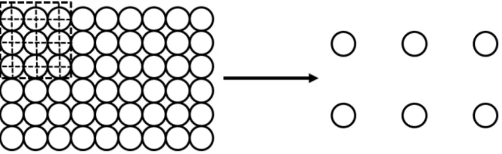
The Kadanoff procedure, often called the block-spin method, is a lattice procedure. It is also the primary method that we use since we make specific calculations involving various Ising models. The procedure is as follows. Start with a large lattice of spins,σr, whereris a vector index labeling the spin’s position in the lattice. The action isS[σ;K], whereKare the coupling constants. The partition function is then,
Z=X
σ
exp(−S[σ;K]). (3.1)
Next, group neighboring spins together. These spins form a block. The block can be formed in all sorts of ways. For example, if we grouped nearest neighbor spins together in a block around a spin at site
r, then the grouped spins would consist ofσrand the spins located one lattice unit away from it; since the nearest neighbors are in the block, the block will look like a diamond.
in the block,σr0 =average of all the spins in a block centered atσrand consisting ofσrand all spins
located one lattice unit away fromσr. Another possibility is to take the majority spin in the block, aka the majority rule (e.g., if most of the spins were up, then the spin that replaces the block will also be up). So for example,σr0 =the spin that occurred the most frequently in the block centered atσr. If a tie-breaker is needed, the new spin takes a random value of the allowed spin values. See Figure3.1for an example of blocking spins in a 2D lattice.
Figure 3.1: An example of grouping spins into blocks in a 2D lattice. In this particular case of blocking, the blocks are squares and contain nine spins; the center spin is chosen for the block, resulting in a lattice with fewer spins and a greater spacing between spins. Other blocking methods could be chosen, e.g., triangles, and different amounts of spins could be included in the blocks.
The replacing of the spins in the block by one spin can be described as a transformationT[σ0|σ], which is normalized as,
X
σ0
T[σ0|σ] = 1. (3.2)
The transformationT is known as a block-spin transformation. Notice the similarity to a conditional probability distribution. This similarity will be exploited in later sections.
The new effective action is then defined as,
exp(−Sef f[σ0;K0]) =X
σ
T[σ0|σ] exp(−S[σ;K]), (3.3)
same as the old partition function,
Znew =X
σ0
exp(−Sef f[σ0;K0])
=X
σ0 X
σ
T[σ0|σ] exp(−S[σ;K])
=X
σ
exp(−S[σ;K]) =Z.
(3.4)
Because each block of spins was replaced with a single spin (known as a block spin), we now have a lattice of spins that have fewer spins than before. Because the block spins are located at the center of each block, the resulting spins are separated by a larger distance (from center to center), thereby indicating a change of scale to lower energy. Once the spins are replaced with new spin variables, the form of the action can be re-written in terms of the interactions between sitesσ0. Hence, we have new couplingsK0
for these interactions. We now have a new actionS[σ0;K0]that has the same form of interactions as the earlier action but with effective coupling constants and defined on a lattice with fewer sites. This effective action in general will also include higher order interactions than the original action, which can be understood to have had zero coupling constant in the original action.
Continuing our example of using a block centered atr, if the lattice originally had a spacinga, it now has a spacing√2a. The new lattice will be rotated relative to the original lattice. Since the new spins are separated by a larger distance, our description of the spin lattice can be understood as a lower energy effective description in terms of the new spin variablesσ0r.
Aside from a constant (i.e., spin-independent) shift in the action, the only thing that will change in the action is the coefficients in front of the spin operators in the action. The partition function is held fixed, so the physics is the same (alternatively, the constant shift in the action can be absorbed into the partition function, in which case the new partition function will differ from the old by an exponential factor of the constant shift).
3.2 Wilson
The Wilsonian method is a continuum procedure for renormalization. It is not really a different method from the Kadanoff procedure but should be thought of as a continuum limit of the Kadanoff procedure with a particular choice of transformationT. Historically, Wilsonian renormalization was used to find fixed points in an RG flow and thereby find universal behavior [126]. In this section, we will be following the treatment of [24].
Unlike the Kadanoff procedure that is used in position space, the Wilsonian renormalization occurs in momentum space. As with the Kadanoff procedure, one starts with an actionS[Φ;K], whereΦare the original field variables (not necessarily scalar) and theKare the original coupling constants. Using the path integral representation, the partition function is,
Z = Z
DΦ exp(−S[Φ;K]). (3.5)
As before, a transformation must be chosen in order to define the effective action. For the Wilsonian method, variables that represent momenta that are higher than some scaleΛare integrated out, while the variables that represent momenta lower than the scaleΛare left for describing the physics at the lower scaleΛ. An easy way to do this is to first define a cutoff for the momentumΛ0. Then split the fields into fast (χ) and slow modes (φ) as,
Φ(x) = Z
p>Λ
dDp Φ(p)eipx+ Z
p<Λ
dDp Φ(p)eipx≡χ(x) +φ(x). (3.6)
We can then integrate out theχfields to produce the lower energy theory. The transformation looks like,
T[φ|Φ] = Z
We define an effective action as,
exp(−Sef f[φ;K0]) = Z
DΦ T[φ|Φ] exp(−S[Φ;K])
= Z
Dχ exp(−S[φ+χ;K]),
(3.8)
where theK0are again the new coupling constants after re-writing the effective action in terms of local operators. Note that the effective action has a cutoff at the scaleΛbecause momentum betweenΛand Λ0 was integrated out. The effective action therefore describes the physics in terms of lower energy variables, i.e., the scale has been changed. The partition function is again the same,
Znew= Z
Dφ exp(−Sef f[φ;K0])
= Z
DφDχ exp(−S[φ+χ;K])
= Z
DΦ exp(−S[Φ;K]) =Z.
(3.9)
As with the Kadanoff procedure, the action must be re-written in terms of local interactions and effective coupling constantsK0. When doing so, new higher order interactions will generally appear; indeed, all possible higher order terms consistent with the symmetries will appear and so will all lower order terms (including a constant operator-independent term: the identity operator). Also, to return the effective action to its original form and to be able to iterate the Wilsonian procedure to find fixed points, a rescaling of the momenta must be done to return the cutoff to its original valueΛ0. After rescaling, one could even relabel the fieldsφasΦso that the end result is an effective action that looks the same as the original action but with different couplings and additional interactions.
The Wilsonian procedure uses a specific transformationTthat allows the procedure to continually be iterated, which is usually used to find fixed points in the RG flow. The rescaling does not affect the numerical values of the coupling constants, and the form of the action is the same, so there is again a flow in the coupling constants with a change in scale (understanding the new higher order interactions to have had coupling constant of zero in the original action) while the rest of the action remains the same:
Also as with the Kadanoff procedure, a constant, operator-independent term will appear in the effective action. This term can be absorbed into the partition function or left in the effective action to keep the partition function fixed.
3.3 Wilson and the Callan-Symanzik Equation
The conceptual result of Wilsonian renormalization as changing the scale of a theory can be applied to the partition function. Doing so results in an example of a Callan-Symanzik equation. A Callan-Symanzik equation shows how observables change with scale to compensate for changes in the coupling constants of the action as the scale is changed. Callan-Symanzik equations are then useful for solving for the couplings and renormalization factors (like the wave-function renormalization factor) as a function of scale, and we will make use of relating observables to changes in scale when we make use of the KL divergence later.
Let us now see an example of a Callan-Symanzik equation. LetZΛ(g(Λ))be the partition function at scaleΛwith coupling constantsg(Λ). Because the partition function is invariant under scale changes, we must have [24,27],
Λ d
dλZΛ(g) =
Λ ∂
∂Λ|g(Λ)+ Λ
∂g(Λ)
∂Λ
∂ ∂g|Λ
Z(g) = 0. (3.10)
By definition,
β≡Λ∂g(Λ)
∂Λ =
∂g(Λ)
∂log(Λ) (3.11)
is the beta function for the coupling constant. Likewise, the wavefunction renormalization factor,Z, will reappear in the kinetic term after performing a renormalization group transformation, and its logarithmic scale derivative is also labeled as,
γ≡ −1
2Λ
∂log(Z(Λ))
∂Λ =−
1 2
∂log(Z(Λ))
∂log(Λ) , (3.12)
andγis known as the anomalous dimension of the field.
Renormalization of correlation functions changes the correlation functions as,