The
EAGLE
simulations of galaxy formation: the importance
of the hydrodynamics scheme
Matthieu Schaller,
1‹Claudio Dalla Vecchia,
2,3Joop Schaye,
4Richard G. Bower,
1Tom Theuns,
1Robert A. Crain,
5Michelle Furlong
1and Ian G. McCarthy
51Institute for Computational Cosmology, Durham University, South Road, Durham DH1 3LE, UK 2Instituto de Astrof´ısica de Canarias, C/ V´ıa L´actea s/n, E-38205 La Laguna, Tenerife, Spain
3Departamento de Astrof´ısica, Universidad de La Laguna, Av. del Astrof´ısico Franciso S´anchez s/n, E-38206 La Laguna, Tenerife, Spain 4Leiden Observatory, Leiden University, PO Box 9513, NL-2300RA Leiden, the Netherlands
5Astrophysics Research Institute, Liverpool John Moores University, 146 Brownlow Hill, Liverpool L3 5RF, UK
Accepted 2015 September 16. Received 2015 September 2; in original form 2015 July 17
A B S T R A C T
We present results from a subset of simulations from the ‘Evolution and Assembly of GaLaxies and their Environments’ (EAGLE) suite in which the formulation of the hydrodynamics scheme is varied. We compare simulations that use the same subgrid models without recalibration of the parameters but employing the standardGADGETflavour of smoothed particle hydrodynamics (SPH) instead of the more recent state-of-the-artANARCHYformulation of SPH that was used in the fiducialEAGLEruns. We find that the properties of most galaxies, including their masses and sizes, are not significantly affected by the details of the hydrodynamics solver. However, the star formation rates of the most massive objects are affected by the lack of phase mixing due to spurious surface tension in the simulation using standard SPH. This affects the efficiency with which AGN activity can quench star formation in these galaxies and it also leads to differences in the intragroup medium that affect the X-ray emission from these objects. The differences that can be attributed to the hydrodynamics solver are, however, likely to be less important at lower resolution. We also find that the use of a time-step limiter is important for achieving the feedback efficiency required to match observations of the low-mass end of the galaxy stellar mass function.
Key words: methods: numerical – galaxies: clusters: intracluster medium – galaxies: forma-tion – cosmology: theory.
1 I N T R O D U C T I O N
Cosmological hydrodynamical simulations have started to play a major role in the study of galaxy formation. Recent simulations are able to cover the large dynamical range required to study the large-scale structure dominated by dark matter as well as the centres of haloes where baryon physics dominates the evolution. Compar-isons of such simulations with observations show broad agreement and help confirm the predictions of the CDM paradigm (e.g. Vogelsberger et al.2014; Schaye et al.2015).
Galaxy formation involves a mixture of complex processes and the numerical requirements to simulate that all of the relevant scales are enormous. A direct consequence of this is the need to model some of the unresolved processes with subgrid prescriptions. Other processes, taking place on larger scales, can in principle
E-mail:[email protected]
be followed accurately by numerical hydrodynamics solvers. The shocking of cold gas penetrating haloes and the turbulence gen-erated by supernova activity within galaxies are examples of the processes that can, in principle, be treated by the hydrodynamics solver. Conversely, the accretion of gas on to black holes and the formation and evolution of stars are examples of processes that occur on scales that are too small to be simulated jointly with the large-scale environment. In practice, however, these two cat-egories of processes are interleaved and it is hence difficult to demonstrate convergence even of the purely hydrodynamical pro-cesses. Practitioners are therefore forced to chose a numerical hy-drodynamics solver that gives accurate results at the resolution of interest.
Many numerical techniques (e.g. Adaptive Mesh Refinement, particle techniques, moving-mesh techniques and mesh-free tech-niques) have been developed over the years to solve the equations of hydrodynamics, each of them coming in different ‘flavours’, i.e. coming with slightly different equations, assumptions and
limitations. For the processes that can be simulated using standard numerical solvers, the main question is how the various parame-ters that enter these hydrodynamics solvers affect the formation of galaxies in the simulations. For example, it has been reported that different numerical techniques and choices of parameters affect the disruption of a cold gas blob in a low-density hot medium, a case di-rectly relevant to the accretion of gas and satellite of galaxies (Frenk et al.1999; Marri & White2003; Okamoto et al.2003; O’Shea et al.
2005; Agertz et al.2007; Wadsley, Veeravalli & Couchman2008; Mitchell et al. 2009; Kereˇs et al.2012; Sijacki et al. 2012). In principle, the values of these numerical parameters can be set by performing controlled numerical experiments for which the solution is known.
In the case of simulations using smoothed particle hydrodynam-ics (SPH) solvers (Lucy 1977; Gingold & Monaghan1977, see Springel2010a; Price2012for reviews), the free parameters relate to the treatment of shocks, artificial viscosity and conduction and are related to the way the SPH equations are derived, leading to dif-ferent flavours of the technique. Performing controlled tests such as Sedov explosions or Kelvin–Helmoltz instabilities (e.g. Price2008; Read, Hayfield & Agertz2010; Springel2010b; Hu et al.2014; Hopkins2015; Beck et al.2015) enables the simulator to identify well-motivated values for the parameters and understand the limi-tations of the formulation. Early flavours of SPH had issues dealing with discontinuities in the fluid. One of many examples of this prob-lem is the ‘blob test’ of Agertz et al. (2007) which was widely used in the literature to demonstrate the failure of SPH. A lot of effort has then been spent by the community to improve the situation and many alternative solutions have been proposed to overcome the ap-pearance of spurious surface tension that prevents the correct mixing of phases. Solutions using either an alternative formulation of the equations in which the discontinuities are smoothed were proposed (e.g. Ritchie & Thomas2001; Read et al.2010; Abel2011; Saitoh & Makino2013) as well as solution involving additional terms dif-fusing material across the discontinuities (e.g. Price2008). Both types of solutions to the discontinuity problem present shortcom-ings (see discussion at the end of Section 2.2) and this motivated the implementation of SPH used in this paper, which uses a combi-nation of both solutions. Although one can in principle calibrate the free parameters using tests, it is unclear whether there is a single set of values that is suitable for all problems and whether these parameter values are also the best choice when performing simula-tions of very hot and diffuse condisimula-tions, such as those present in the hot haloes of galaxies (e.g. Sembolini et al.2015). Moreover, the large gap in resolution between these controlled experiments and cosmological simulations makes the extrapolation of the solver’s behaviour a difficult and uncertain task. The correct treatment of entropy jumps across shocks or of the spurious viscosity that can appear in differentially rotating discs can have direct consequences for the population of simulated galaxies.
In their comprehensive study of galaxy formation models, Scannapieco et al. (2012) used multiple hydrodynamics solvers coupled to multiple sets of subgrid models to simulate the forma-tion of galaxies in a single halo and to study the relative impact of the choice of solver and subgrid model. One of their main find-ings was that the variations in the hydrodynamics solvers led to much smaller changes in the final results than did the changes to the subgrid model parameters. This was especially the case for the prescription of feedback, which can change the final galaxy tremen-dously (e.g. Schaye et al.2010; Haas et al.2013; Vogelsberger et al.
2013; Crain et al.2015). A more controlled experiment was per-formed by Kereˇs et al. (2012), who compared two hydrodynamics
solvers but used only a simplified model of galaxy formation and, apart for the most massive galaxies, found very little difference in the galaxy population despite the large gap in accuracy between the hydro solvers tested. Their two simulations, however, displayed significant differences in the gas properties, especially in the cold gas fractions. More realistic subgrid models, especially of feedback, are likely to suppress some of these differences.
Building on those studies, we attempt to quantify the impact of the uncertainties in two different implementations of SPH solvers on a simulated galaxy population. TheEAGLEsimulation project (Crain
et al.2015; Schaye et al.2015) uses a state-of-the-art implemen-tation of SPH, calledANARCHY(Dalla Vecchia in preparation, see
also appendix A of Schaye et al.2015) and the time-step limiter of Durier & Dalla Vecchia (2012).EAGLE’s subgrid model parameters
were calibrated to reproduce the observed local Universe population of galaxies. In this study, we vary the hydrodynamics solver. We compareANARCHYto the older Springel & Hernquist (2002) flavour of SPH implemented in theGADGETcode (Springel2005) and
com-pare the resulting galaxy population to the one in the reference
EAGLEsimulation and to those in simulations with weaker/stronger
stellar feedback and to runs without AGN feedback. SinceEAGLE
broadly reproduces the observed galaxy population, our test is espe-cially relevant and enables us to disentangle the effects of the hydro solver from the effects of the subgrid model.
This paper is structured as follows. In Section 2, theEAGLEmodel
and the two flavours of SPH that we consider are described. Section 3 discusses the impact of the hydrodynamics solver on the simulated galaxies, whilst Section 4 presents differences in the gas properties of the haloes. A summary of our findings can be found in Section 5. Throughout this paper, we assume a Planck2013flat CDM cosmology (Planck Collaboration XVI2014) (h=0.6777,b=
0.04825,m=0.307 andσ8=0.8288) and express all quantities
withouthfactors.
2 T H E E AG L E S I M U L AT I O N S
TheEAGLEset consists of a series of cosmological simulations with
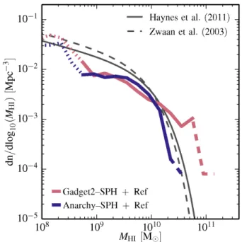
state-of-the-art subgrid models and SPH. The simulations have been calibrated to reproduce the observed galaxy stellar mass function (GSMF), the relation between galaxy stellar mass and supermassive black hole mass and galaxy mass–size relation atz=0.1. The sim-ulations also broadly reproduce a large variety of other observables such as the Tully–Fisher relation and specific star formation rates (SSFRs; Schaye et al.2015), the H2and HIproperties of
galax-ies (Lagos et al.2015, Bahe et al. in preparation), the evolution of the GSMF (Furlong et al.2015), the column density distribution of intergalactic metals (Schaye et al.2015) and HI(Rahmati et al. 2015) as well as galaxy rotation curves (Schaller et al.2015) and luminosities (Trayford et al.2015).
TheEAGLEsimulations discussed in this paper follow 7523≈4.3×
108dark matter particles and the same number of gas particles in a
503Mpc3
cubic volume fromCDM initial conditions. Note that the simulation volumes considered here are a factor of 8 smaller than the main 1003Mpc3
EAGLErun. The mass of a dark matter particle
ismDM=9.7×10⁶Mand the initial mass of a gas particle is
mg=1.8×10⁶M. The gravitational softening length is 700 pc
(Plummer equivalent) in physical units belowz=2.8 and 2.66 kpc (comoving) at higher redshifts. The simulations were run with a heavily modified version of theGADGET-3N-body tree-PM and SPH
impact on the simulation outcome is the topic of this paper. In the next subsections, we will describe the subgrid model used in the
EAGLEsimulations with a special emphasis on those aspects of the
model that are directly impacted upon by the hydrodynamic scheme. For the sake of completeness, we then briefly describe both the standardGADGETandANARCHYflavours of SPH.
2.1 Subgrid models and halo identification
Radiative cooling is implemented using element-by-element rates (Wiersma, Schaye & Smith2009a) for the 11 most important metals in the presence of the cosmic microwave backgroundand UV/X-ray backgrounds given by Haardt & Madau (2001). To prevent artifi-cial fragmentation, the cold and dense gas is not allowed to cool to temperatures below those corresponding to an equation of state
Peos ∝ ρ4/3 that is designed to keep the Jeans mass marginally
resolved (Schaye & Dalla Vecchia2008). Star formation (SF) is implemented using a pressure-dependent prescription that repro-duces the observed Kennicutt–Schmidt SF law (Schaye & Dalla Vecchia2008) and uses a threshold that captures the metallicity dependence of the transition from the warm, atomic to the cold, molecular gas phase (Schaye2004). Star particles are treated as single stellar populations with a Chabrier (2003) initial mass func-tion (IMF) evolving along the tracks provided by Portinari, Chiosi & Bressan (1998). Metals from supernovae and asymptotic giant branch stars are injected into the interstellar medium (ISM) follow-ing the model of Wiersma et al. (2009b) and stellar feedback is implemented by the stochastic injection of thermal energy into the gas as described in Dalla Vecchia & Schaye (2012). The amount of energy injected into the ISM per feedback event depends on the local gas metallicity and density in an attempt to take into account the unresolved structure of the ISM (Crain et al.2015; Schaye et al.
2015). Supermassive black hole seeds are injected in haloes above 1010h−1M
and grow through mergers and accretion of low angu-lar momentum gas (Rosas-Guevara et al.2013; Schaye et al.2015). AGN feedback is performed by injecting thermal energy into the gas directly surrounding the black hole (Booth & Schaye2009; Dalla Vecchia & Schaye2012).
The subgrid model was calibrated (by adjusting the intensity of stellar feedback and the accretion rate on to black holes) so as to reproduce the present-day GSMF and galaxy sizes (Schaye et al.
2015). As discussed by Crain et al. (2015), the latter requirement is crucial to obtain a galaxy population that evolves with redshift in a similar fashion to the observed populations (Furlong et al.2015).
Haloes were identified using the Friends-of-Friends (FoF) algo-rithm (Davis et al.1985) with linking length 0.2 times the mean interparticle distance, and bound structures within them were then identified using the SUBFIND code (Springel et al. 2001; Dolag
et al. 2009). A sphere centred at the minimum of the gravita-tional potential of each subhalo is grown until the mass contained within a given radius,R200, reachesM200=200 (4πρcr(z)R3200/3),
whereρcr(z)=3H(z)2/8πGis the critical density at the redshift of
interest.
2.2 SPH implementations
All simulations that are compared in this study use modifications of theGADGET-3 code. We use both the default flavour of SPH doc-umented in Springel (2005) and the more recent flavour nicknamed
ANARCHY (Dalla Vecchia in preparation; see also appendix A of
Schaye et al.2015) implemented as a modification to the default code. For completeness, we describe both sets of hydrodynamical
equations in this section without derivations. For comprehensive de-scriptions and motivations, see the review by Price (2012) and the description of the alternative formalism by Hopkins (2013,2015). A formulation of SPH that is similar toANARCHY is presented in
Hu et al. (2014). Note that apart from the differences highlighted in this section, the codes (and parameters) used for both types of simulations are identical.
2.2.1 DefaultGADGET-2 SPH
In its default version,GADGET-2 uses the fully conservative SPH
equations introduced by Springel & Hernquist (2002). We will label this ‘GADGETSPH’ in the remainder of this paper and restrict our
discussion of the model to the 3D case. As in any flavour of SPH, the starting point is the choice of a smoothing function to reconstruct field quantities at any point in space from a weighted average over the surrounding particles. In the case of gas density, at positionxi. the equation reads
ρi=
j
mjW(|xi−xj|, hi), (1)
whereW(|r|, h) is the spherically symmetric kernel function. In the case ofGADGET, theM4cubic B-spline function is used and reads
W(r, h)= 8
πh3
⎧ ⎪ ⎪ ⎨ ⎪ ⎪ ⎩
1−6rh2+6rh3 if 0≤r≤h2 21− rh3 if h2 < r≤h
0 if r > h.
The smoothing lengthhiof a particle is obtained by requiring that
the weighted number of neighbours
Nngb=
4 3πh
3 i
j
W(|xi−xj|, hi) (2)
of the particle is close to a pre-defined constant; Nngb = 48 in
our case. Note, however, that contrary to what is often written in the literature,GADGETdefines the smoothing length as the cut-off
radius of the kernel and not as the more physical full width at half-maximum (FWHM) of the kernel function (Dehnen & Aly2012).
The quantity integrated in time alongside the velocities and posi-tions of the particles is the entropic function1A
i=Pi/ρiγ, defined
in terms of the pressurePiand polytropic indexγ. The equations
of motion are then given by
dvi
dt = −
j
mj Pi iρi2∇iWij
(hi)+ Pj
jρ2j∇iWij
(hj)
, (3)
whereiaccounts for the gradient of the smoothing length,
i=1+ hi
3ρi
j
mj∂W∂ijh(hi) (4)
andWij(hi)≡W(xi−xj, hi). In the absence of radiative cooling or thermal diffusion terms, the entropic function of each particle is a constant in time. Only radiative cooling, feedback events (see the previous section) and shocks will change the entropic function.
In order to capture shocks, artificial viscosity is implemented by adding a term to the equations of motion (equation 3) to evolve the
1This quantity is not the thermodynamic entropysbut a monotonic function
entropic function accordingly: dvi
dt
visc= −. 1
4
j
mjij∇Wij(fi+fj)
dAi dt
visc.= 1 8
γ−1
ργ−1 i
j
mjij(vi−vj)· ∇Wij(fi+fj),
withWij ≡(Wij(hi)+Wij(hj)) and the viscous tensor (ij) and
shear flow switchfidefined below. Following Monaghan (1997),
the viscous tensor, which plays the role of an additional pressure in the equations of motion, is defined in terms of the particle’s sound speed,ci=√γ Pi/ρi, as
ij = −α(ci+cρj−3wij)wij
i+ρj , (5)
wij =min
0,(vj−vi)·(xi−xj)
|xi−xj|
(6)
with the dimensionless viscosity parameter set to the commonly used value of α = 2 in our simulations. Finally, to prevent the application of viscosity in the case of pure shear flows, the switch proposed by Balsara (1995) is used:
fi= |∇ ·v |∇ ·vi|
i| + |∇ ×vi| +10−4ci/hi, (7)
with the last term in the denominator added to avoid numerical insta-bilities. The divergence and curl of the velocity field are computed in the standard SPH way (e.g. Price2012).
2.2.2 ANARCHYSPH
The first change inANARCHYwith respect toGADGETis the choice of kernel function. More accurate estimators for both the field quanti-ties and their derivatives can be obtained by using Wendland (1995) kernels (Dehnen & Aly2012).ANARCHYuses theC2kernel. This
ker-nel function is not affected by the pairing instability, which occurs when high values ofNngbare used with spline kernels. It reads
W(r, h)= 21 2πh3
1− rh41+4hr if 0≤r≤h
0 if r > h.
To keep the effective resolution of the simulation similar between the two flavours of SPH, we useNngb=58 with this kernel. This
yields the same kernel FWHM as obtained for the cubic kernel2
withNngb =48. Note, however, that the C2kernel only exhibits
better behaviour than the cubic spline kernel when large numbers of neighbours (Nngb 100) are used (Dehnen & Aly2012). We
use the C2kernel withNngb= 58 to be consistent with both the EAGLEresolution and the hydrodynamics studies of Dalla Vecchia
(in preparation) who used the same kernel but more neighbours. The equations of motion used in theANARCHYflavour of SPH are
based on the pressure–entropy formulation of Hopkins (2013), a generalization of the earlier solutions of Ritchie & Thomas (2001), Read et al. (2010), Abel (2011) and Saitoh & Makino (2013). The two quantities carried by particles that are integrated forward in time are again the velocity and the entropic function. Alongside
2Expressing our resolution in terms of the local interparticle separation
(Dehnen & Aly2012; Price2012) givesη=FWHM(W(r,h))/x=1.235 for both kernels.
the density, which is computed in the usual way (equation 1), two additional smoothed quantities are introduced in this formulation of SPH: the weighted density
¯
ρi= 1 A1/γ
i
j
mjA1j/γW(|xi−xj|, hi) (8)
and its associated weighted pressure, ¯Pi=Aiρ¯iγ. Despite having the same units as the regular density, its weighted counterpart should only be understood as an intermediate quantity entering other equa-tions and should not be used as the gas density. Using these two new quantities, the equation of motion for the particle velocities becomes
dvi dt = −
j mj A
1/γ j A1/γ
i ¯ Pi ¯ ρ2 i
ij∇iWij(hi)
+ A 1/γ i A1/γ
j
¯
Pj
¯
ρ2
jji∇jWij
(hj)
(9)
with the terms accounting for the gradients in the smoothing length reading
ij =1−
1
A1/γi
hi
3ρi
∂P¯1/γ
i
∂hi 1+ hi
3ρi
−1
. (10)
The use of the smoothed quantities ¯Pi and ¯ρi in the equations of motion smooths out the spurious pressure jumps appearing at contact discontinuities in older formulations of SPH (Hopkins2013; Saitoh & Makino2013).
As in all versions of SPH, artificial viscosity has to be added to capture shocks. In theANARCHYformulation of SPH, this is done
following the method of Cullen & Dehnen (2010). Their scheme is the latest iteration of a series of improvements to the standard (Monaghan1997) viscosity term that started with the proposal of Morris & Monaghan (1997) to assign individual viscositiesαito
each particle. Improving on the work of Rosswog et al. (2000), Price (2004) and Wetzstein et al. (2009), Cullen & Dehnen (2010) proposed a differential equation forαithat is solved alongside the
equations of motion (equation 9): ˙
αi=2lvsig,i(αloc,i−αi)/hi, (11)
withl=0.01 and the signal velocityvsig,iintroduced below. The
local viscosity estimatorαloc,iis given by
αloc,i=αmax h 2 iSi v2
sig,i+h2iSi,
(12)
whereαmax=2 andSi=max(0,−ddt(∇ ·vi)) is the shock detector.
After passing through a shock,Si=0 and henceαloc,i=0, leading
to a decrease in αi. We impose αi > αmin = 0.05 to facilitate
particle reordering. The signal velocity is constructed to capture the maximum velocity at which information can be transferred between particles whilst remaining positive:
vsig,i= max |xij|≤hi
1
2(ci+cj)−min(0,vij·xˆij)
, (13)
with ˆxij =(xi−xj)/|xi−xj|andvij=vj−vi.
The individual viscosity coefficients αi are then combined to
enter the equations of motion in a similar way as in theGADGET
formulation. Equations (5) and (6) are replaced by
ij = −αi+αj
2
(ci+cj−3wij)wij
wij =min
0,
vj−vi·(xi−xj)
|xi−xj|
. (15)
Note that contrary to Hu et al. (2014), we do not implement expen-sive matrix calculations (Cullen & Dehnen2010) for the calculation of the velocity divergence time derivative entering the shock detec-torSi as we found that using the standard SPH expressions was
sufficient for the accuracy we targeted.
The last improvement included in theANARCHYflavour of SPH
is the use of some entropy diffusion between particles. SPH is by construction non-diffusive (e.g. Price2012) and does, hence, not in-corporate the thermal conduction that may be required to faithfully reproduce the micro-scale mixing of gas phases. We implement a small level of numerical diffusion following the recipe of Mon-aghan (1997) and Price (2008). We compute the internal energies from the entropies and these are then used in the equations for the diffusion. The use of the pressure–entropy formalism (equation 9) prevents the formation of spurious surface tension at contact discon-tinuities (Hopkins2013). This small amount of numerical diffusion allows the particles to mix their entropies at the discontinuity and hence create one single phase (Dalla Vecchia in preparation). The diffusion is hence used to solve a numerical problem and not to introduce a macroscopic conduction. This results in cluster entropy profiles in agreement with the results from grid and moving-mesh codes (see the comparison of Sembolini et al.2015, which includes
ANARCHY). We compute the rate of change of the conduction using
the second derivative of the energy. This means that large conduction valuesαdiffare triggered by discontinuities in the first derivative of
the energy, not by smooth pressure gradients as in (self-)gravitating objects. Moreover,αdiffmay take some time to increase while the
smoothing of the discontinuity decreases its rate. Finally, our rate is lowered to only a few per cent of the computed value for the value of the free parameterβemployed, contrary to almost all the imple-mentations in the literature. This largely reduces spurious pressure waves. More specifically, the equation describing the evolution of the entropy includes a new term,
dAi dt
diff=. 1
¯
ργ−1
j
αdiff,ijvdiff,ijρmj i+ρj
¯
Pi
¯
ρi −
¯
Pj
¯
ρj
Wij, (16)
with the diffusion velocity given by vdiff,ij =max(ci+cj+
(vi−vj)·(xi−xj)/|xi−xj|,0) and the diffusion coefficient by
αdiff,ij = 12(αdiff,i+αdiff,j). The individual diffusion coefficients are
evolved alongside the other thermodynamic variables following the differential equation
˙
αdiff,i=βhi∇ 2
i( ¯Pi/(γ−1) ¯ρi)
¯
Pi/(γ−1) ¯ρi
, (17)
where, as discussed above, we adoptβ=0.01. We further impose 0< αdiff,i<1, but note that the upper limit is rarely reached, even
for large discontinuities.
2.3 Thermal energy injection and time-step limiter
A crucial aspect of the stellar feedback implementation used in
EAGLEand described in Dalla Vecchia & Schaye (2012) is the
in-stantaneous injection of large amounts of thermal energyuin the ISM. This injection is performed by raising the temperature of a gas particle byT =107.5K, a value much larger than the
aver-age temperature of the warm ISM. In theGADGETformulation of
SPH, this is implemented by changing the entropyAiof a particle.
In the case ofANARCHY, the situation is more complex since the
densities themselves are weighted by the entropies, which implies that a change in the entropy will affect both quantities entering the equations of motion of all the particles in a given neighbourhood. Hence, changing the internal entropy of just one single particle will
notlead to the correct change of energy (across all particles in the simulation volume) of the gas. The thermal energy injected in the gas will be different (typically lower) from what is expected by a simple rise inAi, leading to a seemingly inefficient feedback event.
This problem is alleviated in theEAGLEcode by the use of a series
of iterations during which the values ofAiandρiare changed until
they have converged to values for which the total energy injection is close to the imposed value:
Ai,n+1=
(γ−1)(uold+u)
¯
ργ−1 i,n
,
¯
ρi,n+1=
¯
ρi,nA1n/γ−miW(0, hi)Ai,n1/γ+miW(0, hi)A1i,n/γ+1 A1/γi,n+1
.
This approximation is only valid for reasonable values ofuand only leads to the injection of the correct amount of energy if the energy is injected into one particle in a given neighbourhood, as is the case in most stellar feedback events. This scheme typically leads to converged values (at better than the 5 per cent level) in one or two iterations. When large amounts of energy are injected into multi-ple neighbouring particles, as can happen in some AGN feedback events, this approximation is not sufficient to properly conserve energy (across all particles in a given kernel neighbourhood). To avoid this, we limit the number of particles being heated at the same time to 30 per cent of the AGN’s neighbours. If this threshold is exceeded, the time step of the BH is decreased and the remaining energy is kept for injection at the next time step. Isolated explosion tests have shown that this limit leads to the correct amount of energy being distributed.
As was pointed out by Saitoh & Makino (2009), the conservation of energy in SPH following the injection of large amounts of energy requires the reduction of the integration time step of the particles receiving energy as well as those of its direct neighbours. This was further refined by Durier & Dalla Vecchia (2012), who demonstrated that energy conservation can only be achieved if the time step of the particles is updated according to their new hydrodynamical state. This latter time-step limiter is applied in both theGADGET-SPH and ANARCHY-SPH simulations used in Sections 3 and 4 of this paper.
We discuss its influence on galaxy properties in Subsections 3.1 and 3.2.
3 G A L A X Y P O P U L AT I O N A N D E VO L U T I O N T H R O U G H C O S M I C T I M E
As discussed by Schaye et al. (2015) and Crain et al. (2015), the subgrid models of stellar and AGN feedback are only an incom-plete representation of the physical processes taking place in the unresolved multiphase ISM. In particular, because radiative losses and momentum cancellation associated with feedback from SF and AGN in the multiphase ISM cannot be predicted from first princi-ples, the simulations cannot make ab initio predictions for the stellar and black hole masses. In a fashion similar to the semi-analytic mod-els, the subgrid models for feedback in theEAGLEsimulations have
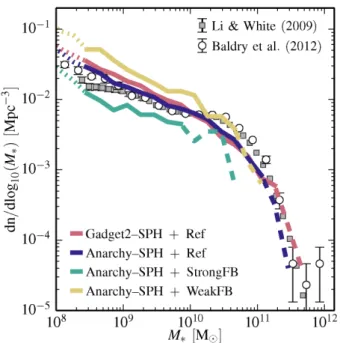
Figure 1. The z = 0.1 GSMF of the L050N0752 simulations using
ANARCHY-SPH (blue line, the EAGLEdefault) andGADGET-SPH (red line).
Curves are drawn with dotted lines where galaxies are comprised of fewer than 100 star particles, and dashed lines where the GSMF is sampled by fewer than 10 galaxies per 0.2 dex mass bin. Data points show measurements with 1σ error bars from the SDSS (Li & White2009, filled squares), and GAMA (Baldry et al.2012, open circles) surveys. The yellow and green lines show the GSMF of the L025N0376 simulations with twice weaker and twice stronger feedback from SF respectively, in a smaller 253Mpc3
volume. The differences due to the choice of hydrodynamics scheme are smaller than the differences due to uncertainties in the subgrid modelling.
galaxy population when the hydrodynamic scheme is reverted to the commonly usedGADGET-SPH formalism. We will specifically focus on the GSMF and galaxy sizes before turning towards the star formation rates (SFRs).
We stress that the model parameters have not been recalibrated when switching our hydrodynamics scheme back toGADGET-SPH.
3.1 The GSMF
In Fig. 1, we show the GSMF atz=0.1 computed in spherical apertures of 30 kpc around the centre of potential of the haloes. As discussed by Schaye et al. (2015), this choice of aperture gives a simple way to distinguish the galaxy and the intra-cluster light. The blue and red lines correspond to our simulations with theANAR -CHYandGADGETflavours of SPH, respectively. We use dashed lines
when fewer than 10 objects populate a (0.2 dex) stellar mass bin and dotted lines when the galaxy mass drops below our resolution limit (for resolution considerations, see Schaye et al.2015). The two hy-drodynamic schemes lead to very similar GSMFs with significant differences only appearing atM∗>2×10¹¹M
, where the small number of objects in the volume prevents a strong interpretation of the deviation, based solely on that diagnostic. The white circles and grey squares correspond to the observationally inferred GSMFs from the GAMA (Li & White2009) and SDSS (Baldry et al.2012) surveys, respectively. The two simulated galaxy populations under-shoot the break of the stellar mass function by a similar amount and are in a similarly good agreement (0.2 dex) with the data. The choice of hydrodynamic solver seems to only impact the mass and abundance of the most massive galaxies in our cosmological
simulations. We reiterate that there has been no recalibration of the subgrid parameters between theGADGETandANARCHYsimulations.
In order to compare the contribution of hydrodynamics uncer-tainties to the unceruncer-tainties arising from the subgrid models, we show using green and yellow lines two additional models using the
ANARCHYflavour of SPH but with feedback from SF injecting half
and twice as much energy, respectively. These simulations are the models WeakFB and StrongFB introduced by Crain et al. (2015) and reduced or increased the number of feedback events taking place, whilst keeping the amount of energy injected per event con-stant. They have been run in smaller volumes (253Mpc3
), leading to poorer statistics at the high-mass end. These changes in the amount of energy injected in the ISM lead to much larger differences in the GSMF than changing the flavour of SPH used for the simulation.
The large impact of variations of the subgrid model for stel-lar feedback on the simulated population and on single galaxies can also be appreciated from the large range of outcomes of the different models in the OWLS suite (Schaye et al.2010; Haas et al.2013) and
AQUILAprojects (Scannapieco et al.2012). Our work, however, uses
a higher resolution than was accessible in the OWLS suite forz=0 and contrary to AQUILAuses a cosmological volume and can hence
study the effect of the hydrodynamics scheme from dwarf galaxies to group-sized haloes. The study of Kereˇs et al. (2012), which com-pared theAREPO(Springel2010b) andGADGET-SPH hydro solvers but using simple subgrid models, came to the same conclusion: the choice of hydrodynamics scheme has little impact on the stel-lar mass function of simulated galaxies at intermediate mass, only the most massive objects are affected. Interestingly, the differences they observed in high-mass galaxies are exactly opposite to our findings: the more accurate solver (in their caseAREPO) produces
more massive galaxies than the simulation usingGADGET-SPH. This confirms that the source terms arising from the physical modelling of the unresolved processes in the ISM, especially the modelling of AGN feedback (see the discussion below in Section 4.2), clearly dominate the uncertainty budget.
We now turn to the impact of the time-step limiter on the sim-ulated galaxy population. As was demonstrated by Durier & Dalla Vecchia (2012), the absence of a time-step limiter leads to the non-conservation of energy during feedback events. The energy of the system after the injection is larger than expected. This implies that a simulation without time-step limiter will have a spuriously high-feedback efficiency. In order to test this, we ran a simulation in a 253Mpc3
volume using the Ref subgrid model and theANARCHY
-SPH scheme but with the Durier & Dalla Vecchia (2012) time-step limiter switched off. Since this simulation volume is too small to be representative, it is more informative to study the relation between halo mass and stellar mass.
In Fig.2, we therefore show the relation between halo mass (M200)
and galaxy formation efficiency (M∗/M200) for central galaxies at z=0.1. As for all other figures, the blue and red lines correspond to theANARCHY-SPH andGADGET-SPH simulations, respectively, both
Figure 2. The median ratio of the stellar and halo mass of central galax-ies, as a function of halo massM200and normalized by the cosmic baryon
fraction atz=0.1 for both the L050N0752ANARCHY-SPH (blue line) and
GADGET-SPH (red line) simulations. Curves are drawn with dashed lines where the GSMF is sampled by fewer than 10 galaxies per bin. The 1σ scatter about the median of theANARCHYrun is denoted by the blue-shaded region. The solid and dashed grey lines show the multi-epoch abundance matching results of Behroozi, Wechsler & Conroy (2013) and Moster, Naab & White (2013), respectively. The yellow and green lines show the GSMF of the L025N0376 simulations with twice weaker and twice stronger feedback from SF, respectively. The cyan line corresponds to the simulation using theANARCHYformulation of SPH and the reference subgrid model, but
with-out the time-step limiter. The absence of the time-step limiter artificially increases the efficiency of the feedback and has a greater impact than the choice of hydro solver.
SF in that simulation, as expected from the analysis of Durier & Dalla Vecchia (2012). This is a purely numerical effect that has to be corrected by the use of small time steps in regions where feedback takes place. The simulation volume considered for that test is too small to contain a large sample of haloes hosting galax-ies with significant AGN activity. Durier & Dalla Vecchia (2012) argued that the larger the energy jump, the larger the violation of energy conservation will be when the time-step limiter is not used. As the energy injection in AGN feedback events is two orders of magnitude larger than for stellar feedback, we expect the masses of galaxies withM∗3×10¹⁰M
(the mass range where AGN feedback starts to be important) to be reduced, compared to the Ref model, even more than the galaxies for which AGN feedback plays no role. Note that the impact of the time-step limiter is much larger than the differences due to the hydrodynamics solver, but smaller than the effect of doubling/halving the feedback strength.
3.2 The sizes of galaxies
Crain et al. (2015) showed that matching the observed GSMF does in general not lead to a realistic population of galaxies in terms of their mass–size relation and mass build-up. Alongside galaxy masses, galaxy sizes were therefore considered in theEAGLEproject
during the calibration of the parameters of the subgrid model for stellar feedback. Crain et al. (2015) demonstrated that numerical
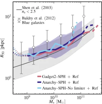
Figure 3. The sizes, atz=0.1, of disc galaxies in the L050N0752ANARCHY
-SPH (blue line) andGADGET-SPH (red line) simulations and in theANARCHY
-SPH model without time-step limiter (cyan line). Size,R50, is defined as the
half-mass radius of a S´ersic profile fit to the projected, azimuthally aver-aged stellar surface density profile of a galaxy, and those with S´ersic index
ns<2.5 are considered disc galaxies. Curves show the binned median sizes,
and are drawn with dotted lines below a mass scale of 600 star particles, and using a dashed line style where sampled by fewer than 10 galaxies per 0.2 dex mass bin. The 1σ scatter about the median of theANARCHYrun is denoted by the blue-shaded region. The solid grey line and the grey shading show the median and 1σscatter of sizes forns<2.5 galaxies inferred from
SDSS data by Shen et al. (2003), whilst white circles with error bars show sizes of blue galaxies inferred by Baldry et al. (2012) from GAMA data. All simulations reproduce thez=0.1 galaxy sizes.
limitations tend to make feedback from SF less efficient at quench-ing the galaxies if the feedback occurs in dense regions of the ISM. This would lead to galaxies that are too compact and with an SSFR at low redshift that is lower than observed. As a consequence, they also showed that selecting model parameters that lead to galaxies with sizes in agreement with observational data was necessary to obtain a realistic population of galaxies across cosmic time. As-sessing the dependence of the galaxy sizes on the hydrodynamics scheme is, hence, crucial.
In Fig.3, we show the sizes of the galaxies in both theANARCHY
-SPH andGADGET-SPH simulations. The observational data sets from
Shen et al. (2003, SDSS, grey line and shading) and Baldry et al. (2012, GAMA, white circles) are shown for comparison. The sizes of the simulated galaxies are computed following McCarthy et al. (2012). We fit a S´ersic profile to the projected, azimuthally averaged surface density profiles. We then extract the half-mass radius of the galaxy,R50, from this profile when integrated to infinity. To match
the observational selection of Shen et al. (2003), we select only galaxies that have a S´ersic indexns< 2.5. We use dashed lines
where the (0.2 dex) mass bins contain fewer than 10 objects and dotted lines for galaxies that are represented by fewer than 600 star particles. The 1σscatter around the mean in theANARCHY-SPH
simulation is shown as the blue-shaded region for the mass bins that are both well resolved and well sampled. The GADGET-SPH
Both simulations reproduce the observed galaxy size–mass re-lation. The simulated galaxies lie within 0.1-0.2 dex of either of the two data sets. As was the case for the GSMF, the galaxy sizes are unaffected by the specific details of the hydrodynamics scheme. This implies that the two hydro schemes have similar energy losses in dense gas regions where feedback takes place. Differences much larger than this can be seen when the subgrid model parameters are varied, even if one requires the GSMF to match observations (Crain et al.2015). Galaxies withM∗>1011M
display small, but not statistically significant, differences with the objects in theGADGET
simulation being slightly smaller. This is in agreement with the findings of Naab et al. (2007) who, usingGADGET-SPH, produced
massive galaxies too compact compared to observations.
When considering the galaxy masses, we found that not using the Durier & Dalla Vecchia (2012) time-step limiter led to an increase of the feedback efficiency, although the magnitude of the effect was small compared to that of doubling the feedback energy. As galaxy sizes were our second diagnostic, we also consider the effect of switching off this limiter on the sizes of our simulated galaxies. This model is shown as the cyan line in Fig.3. The oscillations seen in the curve are due to the smaller volume used for this simulation. The sizes of the galaxies are very close to or slightly larger than the ones in the default simulation.
Crain et al. (2015) also showed that using more efficient stellar feedback leads (among other things) to higher SSFRs, lower passive fractions and lower metallicities. We have verified that turning off the time-step limiter has the same qualitative effects, although the differences are small. We will not consider the effect of turning off the limiter further in the rest of this paper.
3.3 The SFRs of galaxies
We now turn to the SFRs of galaxies. This quantity was not used in the parameter calibration process of theANARCHY-SPH run (i.e.
the defaultEAGLEmodel) and is an important independent
diagnos-tic of the success of the simulation. Furthermore, since the ISM dictates the SFRs of galaxies, changes in the way the equations of hydrodynamics are solved may lead to changes in the SFRs.
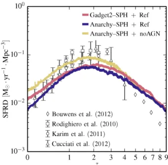
In Fig.4, we show the average SFR per unit volume. The blue and red lines again correspond to theANARCHYandGADGETflavours of SPH, respectively. Observational data from Rodighiero et al. (2010), Karim et al. (2011), Cucciati et al. (2012) and Bouwens et al. (2012) are also shown. Where applicable, the data have been corrected for our adopted cosmology and IMF as described in Furlong et al. (2015). In agreement with the data, both simula-tions display a rise in the SFR density at high redshifts and a fall atz2. As was discussed by Furlong et al. (2015), the constant offset in SFR of≈0.2 dex between the simulations and observa-tions leads to 20 per cent less stars being formed over the cosmic history, consistent with thez=0.1 GSMF (Fig.1), whose ‘knee’ the simulations slightly undershoots.
The simulation using theGADGETversion of SPH predicts a higher
cosmic SFR density than itsANARCHYcounterpart between redshifts
2 and 6 but this does not lead to a large difference in stellar mass formed byz=2. However, the higher SFR seen atz <1 is important and the smaller decrease betweenz=1 and 0 implies an SFR that is 65 per cent higher byz=0 in the simulation using theGADGET
formulation of SPH. This higher SFR can be tentatively related to the larger number of high-mass galaxies seen in the GSMF of this simulation and could, hence, indicate a lower quenching efficiency of the AGN activity in the largest haloes. An extreme version of a model with a low quenching efficiency in large haloes is given by
Figure 4. The evolution of the cosmic SFR density in both the L050N0752
ANARCHY-SPH (blue line) andGADGET-2 SPH (red line) simulations. The
data points correspond to observations from Karim et al. (2011, radio), Rodighiero et al. (2010, 24µm), Cucciati et al. (2012, FUV) and Bouwens et al. (2012, UV). The decline in the SFR density fromz=2 to 0 is less pronounced in theGADGETrun, leading to a 65 per cent higher SFR density atz=0. For comparison, a model without AGN feedback (yellow line) is shown. The SFR density in that model has a low-redshift slope similar to that of theGADGETsimulation.
a model without AGN feedback. Such a model, using theANARCHY
flavour of SPH, is shown using the yellow line in Fig.4. The excess SF at z < 2 is much larger than in the GADGET-SPH based run
with AGN feedback, but the slope is similar and not steep enough compared to the data.
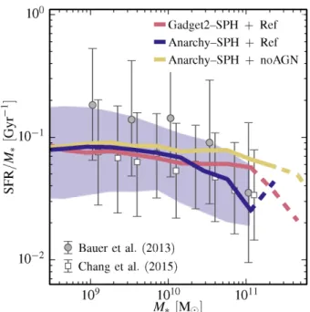
Whether the excess SFR at low redshift is due to large haloes can be confirmed by looking at the SSFR of the simulated galaxies. This quantity is shown in Fig.5as a function of stellar mass. We limit our selection to star-forming galaxies by excluding objects with ˙M∗/M∗<0.01 Gyr−1. As was the case for the stellar mass of
the galaxies, we measure the SFR within a 30 kpc spherical aper-ture. The red and blue lines show the mean SSFR in the simulations using theGADGETandANARCHYflavours of SPH, respectively. As for
other figures, the lines are dashed when a given mass bin is sampled by fewer than 10 objects. The blue-shaded region indicates the 1σ scatter in theANARCHY-based simulation. TheGADGET-based
simula-tion displays a scatter of the same magnitude. For comparison, we show the SSFR inferred from observations in the GAMA survey by Bauer et al. (2013, grey circles) and observations by Chang et al. (2015) using recalibrated SFR indicators based on SDSS+WISE
photometry (white squares). Simulated galaxies with massesM∗∼
1011M
are in agreement with the Bauer et al. (2013) data, whilst lower mass objects exhibit a SSFR lower than observed with the dis-crepancy reaching∼0.3 dex atM∗∼109M
. Schaye et al. (2015) showed that part of this discrepancy goes away if the resolution of the simulation is increased. Interestingly, the recalibrated SF tracers of Chang et al. (2015) lead to lower SSFRs in excellent agreement with theEAGLEresults. Both theGADGETandANARCHYsimulations
show the same behaviour at low masses.
At the upper end of the mass spectrum the two simulations do, however, differ. The SFR of galaxies withM∗2×10¹⁰M
Figure 5. The median SSFR ˙M∗/M∗, of star-forming galaxies ( ˙M∗/M∗> 0.01 Gyr−1) as a function of stellar mass atz=0.1 in the L050N0752 ANARCHY-SPH (blue line) andGADGET-2 SPH (red line) simulations. Dashed line styles are used where the simulation is sampled by fewer than 10 galaxies per 0.2 dex mass bin. The 1σ scatter about the median of theANARCHYrun is denoted by the blue-shaded region. Observational data points with error bars correspond to the median and 1σscatter of the SSFR from GAMA by (Bauer et al.2013, grey circles) and SDSS+WISEby (Chang et al.2015, white squares). Galaxies withM∗>2×10¹⁰Mhave a significantly higher SSFR in theGADGET-SPH simulation than in theANARCHY-SPH one, but the decrease is smaller than when AGN activity is turned off (yellow line).
significantly larger for theGADGETformulation of SPH. AtM∗∼
1011M
, the discrepancy is 0.3 dex.
Complementary to the SSFR of the star-forming galaxies, the passive fraction provides a good diagnostic of the efficiency with which SF is quenched in large galaxies This quantity is shown in Fig.6for both our simulations. Galaxies are considered passive if their SSFR is smaller than 0.01 Gyr−1, which is an order of
mag-nitude below the observed median SSFR for star-forming galaxies at that redshift. For comparison, the data points show the fractions inferred from SDSS data by Gilbank et al. (2010) and Moustakas et al. (2013). We only show points for the simulated population at masses for which there are at least 100 particles at the median SSFR (see Schaye et al.2015).
The two simulations present a very different behaviour for galax-ies withM∗2×10¹⁰M
. Whilst theANARCHY-SPH simulation follows the trend seen in the observational data, theGADGET-SPH
simulation shows a constant passive fraction of ∼15 per cent at masses up toM∗=2×10¹¹M
. At larger masses, the fraction is 0, implying that all galaxies are star forming, in disagreement with the data that indicates that almost all galaxies (>80 per cent) of that mass range are passive. Note, however, that there are only 20 galaxies withM∗>1011M
in the simulation volume and that the fractions displayed in Fig.6are, hence, affected by small number statistics. Since theANARCHYandGADGETsimulations use the same initial conditions, the comparison between the two schemes is, how-ever, still meaningful. Switching fromANARCHYto standardGADGET
has qualitatively a similar effect as switching off AGN feedback (yellow line).
Figure 6. The fraction of passive galaxies ( ˙M∗/M∗<0.01 Gyr−1) at
z =0.1 in both the L050N0752ANARCHY-SPH (blue line) andGADGET
-SPH (red line) simulations. We only show mass bins that correspond to 100 or more star-forming particles for the median SSFR. The grey circles and white squares correspond to the passive fractions inferred from the SDSS data by Gilbank et al. (2010) and by Moustakas et al. (2013). The passive fraction is far too low for galaxies withM∗2×10¹⁰M
in theGADGET
simulation, in a similar fashion to theANARCHYsimulation without AGN
feedback (yellow line).
The shortage of passive galaxies in theGADGETsimulation at the
high-mass end of the galaxy population and the higher SSFR for high-mass objects both indicate that the SF quenching processes are inefficient in the largest haloes. This higher SFR at low redshift in high-mass haloes leads to an increase of the stellar mass of massive galaxies as was hinted at by the difference in the GSMFs between the two simulations atz=0.1 (Fig.1). AGN feedback, which is the main source of quenching in our model for galaxies withM∗ 2×10¹⁰M
, seems to be insufficiently effective at quenching SF in large haloes in theGADGETsimulation.
It is worth mentioning that we cannot eliminate the possibil-ity that a recalibration of the subgrid parameters could bring the
GADGETsimulation into agreement with the data. By changing the
frequency of the AGN events or the temperature to which the gas is heated during such an event, it might be possible to quench SF in large galaxies even when theGADGETformulation of SPH is used.
It is, however, unclear if this could be achieved and whether sub-grid parameters should be used to compensate for the shortcomings of a particular hydro scheme. Similarly, simulations run at differ-ent resolutions might lead to differdiffer-ent conclusions (if the subgrid parameters are kept fixed). Note that simulations run at a lower resolution (such as the low-redshift versions of OWLS Schaye et al.
2010and cosmo-OWLS Le Brun et al.2014) have fewer resolution elements in the haloes and may hence not suffer as much from the lack of phase mixing (see discussion below). A full exploration of the subgrid model parameter space or a comprehensive resolution study is, however, beyond the scope of the present paper.
from which stars can be formed in those haloes. The AGN will sustain a hot halo in which these filaments will dissolve. It is likely that the spurious surface tension that plagues the density–entropy formulation of SPH used inGADGETdoes not leave the gas in the hot
halo in a state where the AGN activity can be effective at stopping SF. An example of these issues would be the inability for dense gas blobs to dissolve in a hot halo medium (see for instance the ‘blob test’ problem by Agertz et al.2007), which could allow cold pristine gas in filaments to survive the hot bubbles created by the AGN activity and feed the galaxy with gas ready to form stars. The better phase-mixing ability of theANARCHYformulation of SPH is more
effective at disrupting infalling filaments and prevent them from reaching the galaxies, making the AGN-driven bubbles effective at stopping SF. In this scenario, the issue is not that outflows generated by an AGN are unable to sustain a hot halo (we will show that hot haloes are present in both cases), it is rather the pristine gas that forms clumps that are unstable and cool rather than being mixed in. The next section further explores the differences in gas properties of the two simulations.
4 L A R G E - A N D S M A L L - S C A L E G A S D I S T R I B U T I O N
In the previous section, we showed that the masses and sizes of galaxies are only marginally affected by the improvements to the hydrodynamics scheme made in theANARCHYflavour of SPH. We also showed, however, that the SFRs of massive galaxies are signif-icantly affected by these same improvements and argued that some of the differences might be directly related to the way in which the different SPH schemes treat the gas in large haloes. In this section, we explore this possibility by studying the state of the gas both out-side and inout-side haloes. We will focus on the largest systems, where the dynamical time is similar to or shorter than the cooling time of the hot gas, and hence the hydrodynamic forces become important.
4.1 Gas in large-scale structures
A simple diagnostic of the state of the gas in a simulation is the dis-tribution of the SPH particles or grid cells in the density-temperature plane. The different components (ISM, IGM, etc.) can then be iden-tified and their relative abundance in terms of mass or volume estimated. Since theANARCHYandGADGETformulations behave dif-ferently when different phases are in contact or in the presence of a shock, it is worth analysing the differences created by those schemes. In order to minimize the impact of the subgrid models on the distribution of the gas, we start by looking at the gas in the interhalo medium, i.e. the gas outside of haloes. Most of the gas that is located outside of haloes has had little contact with star-forming regions or with the winds driven by AGN and SF but some of the material might have been enriched early on in protohaloes (e.g. Oppenheimer et al.2012). We are hence focusing on the low-metallicity, mostly primordial, gas before it falls on to haloes. This should allow us to consider differences driven mostly by the two flavours of the hydrodynamics scheme.
The haloes have been identified using the FoF algorithm and are hence typically larger than the commonly given virial radii. This ensures that we are not considering particles that are part of any resolved haloes. In both our simulations, we only identify haloes that have more than 32 particles, effectively imposing a minimum halo mass of MFoF= 3.1×10⁸M. This analysis is resolution
dependent via the definition of the minimum halo mass resolved by the simulation. If the resolution were increased, one would find
smaller haloes, meaning that some of the particles that we identify as being outside of any halo will become part of small haloes. However, small haloes are unlikely to host large amounts of SF and drive enrichment and feedback. As both simulations have been run at the same resolution with the same initial conditions, the same objects will collapse and form haloes, ensuring that our one-to-one comparison is not compromised by the potential presence of smaller unresolved structures.
In Fig.7, we show the distribution of the gas outside of all FoF groups in the density-temperature plane atz=0 forGADGET-SPH
(left-hand panel) andANARCHY-SPH (right-hand panel). The
low-density material (nH<10−4cm−3) is in a very similar state in the
two simulations with an extended distribution of diffuse material spanning more than four orders in magnitude in temperature. The higher temperature material has been heated by feedback activity and blown out of the haloes in both simulations. Differences start to appear at intermediate densities (10−4cm−3< n
H<10−1cm−3).
A lot more mass resides in that regime in the simulation using the
GADGETformulation of SPH. Because of the artificial surface
ten-sion appearing inGADGET-SPH between different phases in contact
discontinuities, this dense gas is unable to properly mix with the lower density, higher temperature material surrounding it. In the
ANARCHYsimulation, the use of both the pressure–entropy
formula-tion of the SPH equaformula-tions and of a (small numerical) diffusion term has allowed this dense gas to dissolve into its surroundings. The dif-ference is even more striking at higher densities (nH>10−1cm−3),
where no gas is present in theANARCHY simulation, whilst a
sig-nificant amount is present in theGADGETone. This difference is
especially important since, depending on its metallicity, some of this dense gas may be star forming. SF is hence taking place outside of collapsed structures in the simulation usingGADGET. Interestingly, this high-density gas also has a high metallicity (Z0.1Z). This gas has thus been ejected from haloes after having been enriched by SF. InANARCHY-SPH, similar material would likely be dissolved
into the surrounding lower density medium, either outside haloes or in winds inside haloes.
4.2 Extragalactic gas in haloes
We find that within haloes differences in the density-temperature diagram are best quantified by looking at the distribution of star-forming gas. We define the IntraGroup Medium (IGrM) as the gas withinR200but outside of 30 kpc masks placed at the centre of
each subhalo. This excludes the gas present in the ISM or close to galaxies and should leave us with a reasonable definition of the IGrM.
In Fig.8, we show the SFR of the IGrM as a function of the halo massM200atz=0.1 for objects extracted from theANARCHY
simulation (blue squares) and theGADGET-SPH simulation (red cir-cles). Haloes with massesM2001012Mhave a higher SFR in
the IGrM in the simulation using theGADGETformulation of SPH
than in theANARCHYsimulation. The higher fraction of dense gas
(nH>10−1cm−3) in theGADGETsimulation leads to a higher IGrM
SFR. The specific SF of the IGrM corresponds to≈5×10⁻³Gyr−1
in theGADGETsimulation and is more than an order of magnitude
lower (≈4×10⁻⁴Gyr−1
) forANARCHY. Although these values are
low when compared to the typical values for galaxies (see Fig.5), the presence of significant SF in the IGrM indicates that the AGN activity or gravitational heating is not effective enough at quenching SF in the largest haloes.
As the haloes in theGADGET-based simulation exhibit more SF
Figure 7. The mass-weighted distribution of gas outside of collapsed structures in the density–temperature plane. The left-hand panel shows thez=0 distribution for theGADGET-SPH simulation, whereas the right-hand panel shows the equivalent distribution for theANARCHY-SPH simulation. TheGADGET-SPH
run displays high-density gas on the imposed equation of state, whilst there is no gas in theANARCHY-SPH run above a density ofnH>10−1cm−3. Dense
star-forming gas is mixing with the lower density, higher temperature medium in theANARCHY-SPH run, whilst the artificial surface tension introduced by the GADGET-SPH formulation prevents this gas from dissolving and leads to SF outside of haloes.
Figure 8. The SFR of the IGrM, i.e. inside the halo but at least 30 kpc from any identified galaxy, as a function of halo mass atz=0.1 for the L050N0752
ANARCHY-SPH (blue squares) andGADGET-SPH (red circles) simulations. The
IGrM is forming significantly more stars in group- and cluster-mass haloes (M200>5×10¹²M) in the run using theGADGET-SPH scheme.
is distributed spatially. To this end, we selected the most massive halo (M200≈2×10¹⁴M) in both simulations and constructed
column density maps of the gas. As we are mainly interested in the dense gas and to increase the clarity of the maps, we only select gas withnH>10−2cm−3. As discussed above, the behaviour of the
warm diffuse medium is similar for both formulations of the SPH equations and can hence be safely discarded here.
These dense gas column density maps are shown in Fig.9for the
GADGET(left-hand panel) andANARCHY(right-hand panel)
simula-tions. The large dashed circles indicate the position of the spherical overdensity radius,R200≈1.1 Mpc, whilst the small solid circles
indicate the innermost 100 kpc, where the effects of the central galaxies on the gas will be maximized. We will not consider this central region in the remainder of this subsection since, as was discussed in Section 3, in this region the differences due to the hy-dro solver are likely to be smaller than the ones induced by small variations in the subgrid parameters.
The difference between the two maps is striking. The halo from theGADGETsimulation contains a large number of dense clumps of
gas at all radii, as was found in the simulations of Kaufmann et al. (2009). These clumps can be seen even inside the inner 100 kpc where feedback from both the AGN and SF might be expected to disrupt them. These nuggets of dense gas also accompany the infalling satellites. The map extracted from theANARCHYsimulation
is much smoother and dense gas is found mostly in the wakes of infalling satellite galaxies following their stripping.ANARCHY’s
ability to mix phases in contact discontinuity allows dense clumps to dissolve into the hot halo, whereas the spurious surface tension that appears between phases inGADGET-SPH allows them to survive
and perhaps even grow. Since some clumps reach densities that exceed the threshold for SF, some of them will increase the SFR of the IGrM. Here, the flavour of SPH has a direct consequence on the observables extracted from the simulation.
Figure 9. Maps of the column density of dense gas (nH>0.01 cm−3) in the largest haloes (M200≈2×10¹⁴M) of the L050N0752GADGET-SPH (left-hand panel) andANARCHY-SPH (right-hand panel) simulations. The large dashed circle shows the location of the spherical overdensity radiusR200, whilst the small
solid circle in the centre encloses the inner 100 kpc. The halo in theGADGET-SPH run contains a large number of dense clumps of gas, as was found by Kaufmann et al. (2009) in their simulations, while its counterpart in theANARCHY-SPH run displays a much smoother gas distribution. The spurious surface tension appearing in theGADGETformulation of SPH makes it difficult for the dense gas stripped from the infalling satellites to be disrupted and mixed into the IGrM.
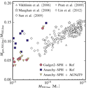
Figure 10. Thez=0 gas fractions withinR500,hseas a function ofM500,hse
inferred from virtual X-ray observations of the L050N0752ANARCHY-SPH (blue squares) andGADGET-SPH (red circles) simulations. Data points cor-respond to measurements from Vikhlinin et al. (2006, triangles), Maughan et al. (2008, stars), Sun et al. (2009, diamonds), Pratt et al. (2009, crosses) and Lin et al. (2012, pentagons). TheANARCHY-SPH Ref model overpredicts the gas fractions for group-sized objects but this can be solved by using the AGNdT9 prescription for AGN feedback (yellow triangles). The haloes of theGADGET-SPH run are in better agreement with the data as a result of their
higher fraction of cold gas that artificially reduces the X-ray inferred gas fractions.
the halo mass and gas fraction following the same analysis that is applied to observational data. For comparison, we show data from Vikhlinin et al. (2006), Maughan et al. (2008), Sun et al. (2009), Pratt et al. (2009) and Lin et al. (2012). We only selected clusters at
z <0.25. As was discussed by Schaye et al. (2015), the simulation using theANARCHYflavour of SPH (blue squares), the Ref model ofEAGLE, overshoots the extrapolated trend seen for higher mass
haloes. This indicates either that the amount of X-ray gas in these haloes is too high or that the gas is in the wrong thermodynamic state. The analysis of a larger simulation volume with more haloes overlapping with the observations motivated Schaye et al. (2015) to introduce an alternative model (labelled AGNdT9) for which the mock-observation inferred gas fractions are in better agreement with the trend in the data. This model uses more sparse, but also more energetic AGN heating events and is shown in Fig.10using yellow triangles.3
Interestingly, theEAGLERef model using theGADGETversion of
SPH (red circles) yields results that are very similar to the improved AGNdT9 model combined withANARCHY-SPH. The gas fractions
are in reasonable agreement with the data. However, the analysis of the dense gas maps and the following discussion indicates that this better agreement is mostly accidental and not a success of the model. The X-ray inferred gas fractions are driven down by a change in the gas mass in the haloes but also by the presence of cold and dense gas in the IGrM that does not emit X-ray and hence artificially reduces the inferred gas masses. The cold clumps lead to the SF seen in Fig.7. We note, however, that these spurious undisrupted clumps
3We note that the map of the column density of dense gas of the largest halo
in this model is very similar to the one using the Ref model and theANARCHY