A Parametric Study of Formation Flight of a Wing Based on Prandtl's Bell-Shaped Lift Distribution

A PARAMETRIC STUDY OF FORMATION FLIGHT OF A WING BASED ON

PRANDTL’S BELL-SHAPED LIFT DISTRIBUTION

A Thesis

presented to

the Faculty of California Polytechnic State University,

San Luis Obispo

In Partial Fulfillment

of the Requirements for the Degree

Master of Science in Aerospace Engineering

By

Kyle Sean Lukacovic

ii

© 2020

Kyle Sean Lukacovic

iii

COMMITTEE MEMBERSHIP

TITLE: A Parametric Study of Formation Flight of a Wing Based

on Prandtl’s Bell-Shaped Lift Distribution

AUTHOR: Kyle Sean Lukacovic

DATE SUBMITTED: June 2020

COMMITTEE CHAIR: Aaron Drake, Ph.D.

Professor of Aerospace Engineering

COMMITTEE MEMBER: Paulo Iscold, Ph.D.

Associate Professor of Aerospace Engineering

COMMITTEE MEMBER: David Marshall, Ph.D.

Professor of Aerospace Engineering, Department Chair

COMMITTEE MEMBER: Russell Westphal, Ph.D.

iv ABSTRACT

A Parametric Study of Formation Flight of a Wing Based on Prandtl’s Bell-Shaped Lift Distribution

Kyle Sean Lukacovic

The bell-shaped lift distribution (BSLD) wing design methodology advanced by Ludwig Prandtl in 1932 was proposed as providing the minimum induced drag. This study used this method as the basis to analyze its characteristics in two wing formation flight. Of specific interest are the potential efficiency savings and the optimal positioning for formation flight. Additional comparison is made between BSLD wings and bird flight in formation.

This study utilized Computational Flow Dynamics (CFD) simulations on a geometric modeling of a BSLD wing, the Prandtl-D glider. The results were validated by modified equations published by Prandtl, by CFD modeling published by others, and by Trefftz plane analysis. For verification, the results were compared to formation flight research literature on aircraft and birds, as well as published research on non-formation BSLD flight.

The significance of this research is two part. One is that the BSLD method has the potential for significant efficiency in formation flight. The optimal position for a trailing wing was determined to be partially overlapping the leading wing vortex core. For a BSLD wing these vortices are located inboard from the wingtips resulting in wingtip overlap and have a wider impact downstream than the elliptical lift distribution (ELD) wingtip vortices. A second aspect is that avian research has traditionally been studied assuming the ELD model for bird flight, whereas this study proposes that bird flight would be better informed using the BSLD.

v

ACKNOWLEDGMENTS

First and foremost, I would like to thank my Dad, John Lukacovic. A father’s love is the compass by which his children learn to navigate, to sail, and to reach their dreams. I would not be here without you. From the bottom of my heart I send my appreciation for all that you do.

I would like to thank Dr. Graham Doig for giving me the opportunity to pursue graduate education at Cal Poly. Without this opportunity and his guidance, I would not be at NASA Ames working as a wind tunnel test director. It is a step or two up from the lab in Building 41 but in the grand scheme of things it operates the same.

I would also like to thank my advisor Dr. Aaron Drake for his patience and time. Their expertise and professionalism in the field of aerospace engineering and knowledge of aerodynamics has propelled my drive to shoot for excellence. His acceptance of the advisor position at an advanced stage in the project reflects his dedication to his students.

I send my deepest gratitude to my distinguished committee members. The feedback I received from Dr. Paulo Iscold, Dr. David Marshall, and Dr. Russell Westphal helped push my thesis. I especially appreciate their willingness to step in and help with my extended thesis process.

I thank Albion Bowers and Oscar Murillo for the experience of a lifetime out in the Mojave Desert where I learned of a little thing called the Bell-Shaped Lift Distribution. My internship sending the Prandtl-D wing soaring into the sky led me to the hypotheses I present herein for the wing in formation flight. This research would not have been published to the world without turning me into a believer of the impossible.

vi

A big shout out also goes Dr. Nancy Squires at Oregon State University. Her classes in aerospace engineering and many long office hour talks persuaded me to reach towards the stars and fly towards a masters in aeronautics.

I also send thanks to two of my best friends and roommates from my time at Cal Poly, Sabir Utamsing and Matt Nguyen. From the countless hours of watching movies with popcorn, to the uncountable hours sitting in the lab trying to determine how to get the schlieren to work, my fondest memories will always be the experiences I shared with them. I can’t wait to see what they do in the future.

To the rest of my family, friends, coworkers, and everyone else who has touched me throughout this journey we call life, I thank you. A whole book can be written for how they have shaped me into the person I am today.

vii

TABLE OF CONTENTS

SECTION PAGE

LIST OF TABLES ... ix

LIST OF FIGURES ... x

NOMENCLATURE ... xii

1. INTRODUCTION ... 1

1.1. Hypotheses ... 2

1.2. Methodology ... 2

2. PREVIOUS WORK ... 4

2.1. The Bell-Shaped Lift Distribution ... 4

2.1.1. Discovering the Minimum Induced Drag Solution ... 4

2.1.2. A Simplification of Prandtl’s Equations ... 12

2.1.3. Additional Minimum Induced Drag Studies ... 14

2.2. Far-Field Induced Drag ... 15

2.3. Prandtl-D Research ... 17

2.4. Birds and Avian Formation Flight ... 20

2.4.1. Beneficial Positioning vs Position Frequency... 24

2.4.2. Induced Drag Reduction ... 25

2.4.3. Optimal Bird Position ... 25

2.4.4. Beneficial Range ... 26

2.4.5. Vortices ... 30

2.4.6. Reported Findings ... 32

2.4.7. Summary – Bird Formation Flight ... 33

2.5. Formation Flight of Aircraft ... 34

2.5.1. Induced Drag Reduction ... 35

2.5.2. Optimal Wing Position ... 35

2.5.3. Beneficial Range ... 36

2.5.4. Vortices ... 37

2.5.5. Summary – Aircraft Formation Flight ... 37

3. THREE-DIMENSIONAL MODELING... 39

3.1. Prandtl-D Geometry ... 39

3.2. Three-Dimensional Point Manipulation ... 41

3.3. CAD Creation ... 42

3.4. Final Geometry ... 44

4. SIMULATION SETUP ... 48

4.1. CFD Software and Resources ... 48

viii

4.3. Fluid Domain ... 50

4.3.1. Trailing Wing Placement ... 51

4.3.2. Domain Sizing ... 52

4.4. Mesh Generation ... 55

4.4.1. Prism Layers ... 55

4.4.2. Grid Convergence Studies ... 57

4.5. Baseline Validation ... 60

5. RESULTS AND ANALYSIS ... 64

5.1. Test Matrix and Convergence ... 64

5.2. Data Processing and Results ... 69

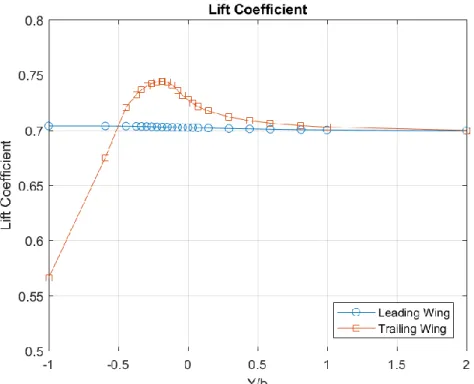
5.2.1. Lift... 71

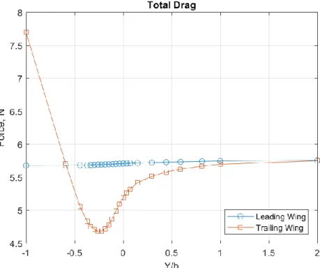
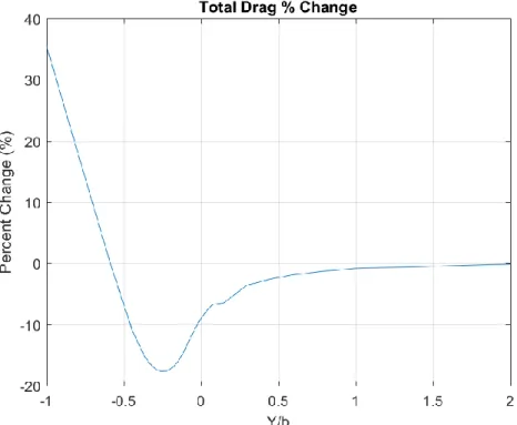
5.2.2. Drag... 73

5.2.3. Lift-to-Drag Ratio ... 76

5.2.4. Skin Friction and Pressure Drag ... 77

5.2.5. Results Summary ... 82

5.3. Trefftz Plane Analysis ... 83

5.4. The Optimal Wing Position and Beneficial Range ... 89

5.5. Pressure Profile Data ... 95

6. CONCLUSION ... 100

6.1. The Bell-Shaped Lift Distribution Benefits ... 100

6.2. The Optimal Wing Position and Beneficial Range ... 101

6.3. Bird Formation Flight ... 102

6.4. Vortices ... 104

6.5. Summary ... 105

REFERENCES ... 106

APPENDICES ... 108

Appendix A ... 108

Appendix B ... 112

Appendix C ... 118

Appendix D ... 159

Appendix E ... 161

Appendix F ... 164

Appendix G ... 171

Appendix H ... 174

ix

LIST OF TABLES

TABLE PAGE

2.1 𝜇 Variation in Relation to Aerodynamic Characteristics Ratios ... 7

2.2 Median and Range for Wingtip Spacing (WTS, in cm) for Canada Geese in Eight Formations ... 27

2.3 Optimal Position and Beneficial Range from Avian Observation ... 34

2.4 Optimal Wing Position, Beneficial Range, and Induced Drag from Aircraft Research 38 3.1 Surface Split Line Locations from Centerline ... 44

3.2 Section Chord Lengths ... 45

3.3 Additional Section Chord Lengths ... 46

3.4 Model Reference Dimensions ... 47

4.1 Domain Sizing Mesh Settings ... 53

4.2 Summary of Three Domain Sizes ... 53

4.3 Fluid Domain Sizing Parameters ... 54

4.4 Change in Forces between Domain Sizes ... 54

4.5 Lift and Drag Values with Increased Mesh Density Close to the Wing ... 57

4.6 Lift and Drag Values with Increased Wake Mesh Density ... 57

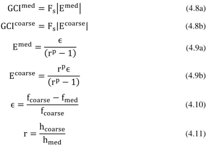
4.7 CGI and Error Values with Increased Mesh Density Close to the Wing... 58

4.8 CGI and Error Values with Increased Wake Mesh Density ... 58

4.9 Mesh Settings Determined from Wing Surface Mesh Convergence Study ... 59

4.10 Additional Mesh Settings Determined from Wake Mesh Convergence Study ... 60

4.11 Differences to Yoo’s Physics Set Up ... 61

5.1 Configuration Domain Sizes ... 67

5.2 Residual Values ... 69

5.3 Percentage of Total Drag for Skin Friction and Pressure Drags ... 78

5.4 Optimal Prandtl-D Position for Various Aerodynamic Parameters ... 82

5.5 Optimal Position and Beneficial Range for Various Aerodynamic Parameters for the Prandtl-D ... 91

5.6 Aerodynamic Parameter Percent Change Between Y/b = 0.148 and -0.444 for the Trailing Wing Compared to the Leading Wing ... 91

5.7 Optimal Elliptical Wing Position and Reduction in System Induced Drag from Various Studies ... 92

6.1 Optimal Prandtl-D Position for Various Aerodynamic Parameters ... 101

x

LIST OF FIGURES

FIGURE PAGE

2.1 Induced drag ratio compared to the circulation ratio ... 8

2.2 Circulation distribution of various spanloads ... 9

2.3 Downwash velocity distribution of various spanloads ... 9

2.4 Flow fields resulting from the elliptical (a. Left) and bell-shaped (b. Right) spanloads ... 10

2.5 Distribution of spanwise local lift ... 13

2.6 Flow on the Trefftz plane behind a lifting body ... 16

2.7 NASA Armstrong’s Prandtl-D P2 in an early flight in 2015 ... 17

2.8 Angular momentum data from an onboard Inertial Measurement Unit on the Prandtl-D wing. The red is pitch rate, blue is roll rate, and green is yaw rate ... 18

2.9 Analytical and experimental downwash and vortex roll-up on the P2 ... 20

2.10 A laysan albatross (phoebastria immutabilis) flying at Kaena Point, O’ahu, Hawaii ... 22

2.11 Common cranes (grus grus) flying in formation over lake Fehér near Sándorfalva, Hungary ... 22

2.12 Formation flight of brown pelicans (pelecanus occidentalis) photographed by Michael Cox ... 23

2.13 Frequency distribution of wingtip spacing for Canada geese (branta canadensis) .... 27

2.14 Frequency distribution of average wingtip spacing of white pelicans (pelecanus erythrorhynchos) in formation flight ... 28

2.15 Frequency distribution of wingtip spacing for Greylag geese (anser anser) ... 29

2.16 Histogram detailing the total number of flaps recorded between each bird–bird pair, with respect to position of the following bird ... 30

2.17 Spedding’s kestrel (falco tinnunculus) trailing vortex location data ... 31

3.1 Plot of nondimensional centerline and wingtip airfoil profiles ... 40

3.2 Wing twist angle as a function of the semispan ... 41

3.3 Imported curves consisting of airfoil profiles, leading edge, and trailing edge ... 42

3.4 Knitted wing surfaces ... 43

3.5 Divided surfaces and section planes ... 43

3.6 Final CAD model ... 44

4.1 Pressure coefficient contours and surface streamlines on the upper surface of the P-3C at 8° AoA ... 50

4.2 Domain boundary settings. (a) Top view and (b) Side view ... 51

4.3 Three view drawing of the fluid domain sizing parameters ... 53

xi

4.5 CL and CD comparison between current baseline and Yoo’s analysis ... 62

4.6 Verification of the spanwise local lift distribution ... 63

5.1 Visualization of Y/b in three configurations (-0.148, 0.000, and 0.148) ... 66

5.2 Number of cells, faces, and vortices once meshed ... 68

5.3 Lift comparison between the leading and trailing wings ... 72

5.4 Lift coefficient comparison between the leading and trailing wings ... 72

5.5 Percent change in lift of the trailing wing compared to the leading wing ... 73

5.6 Total drag comparison between the leading and trailing wings ... 74

5.7 Total drag coefficient comparison between the leading and trailing wings ... 75

5.8 Percent change in total drag of the trailing wing compared to the leading wing ... 75

5.9 Lift-to-drag ratio comparison between the leading and trailing wings ... 76

5.10 Percent change of the lift-to-drag ratio of the trailing wing compared to the leading wing ... 77

5.11 Pressure drag comparison between the leading and trailing wings ... 79

5.12 Percent change in pressure drag of the trailing wing compared to the leading wing 80 5.13 Skin friction drag comparison between the leading and trailing wings ... 80

5.14 Percent change in skin friction drag of the trailing wing compared to the leading wing ... 81

5.15 Total drag, pressure drag, and skin friction drag for the leading and trailing wings . 81 5.16 Induced drag of the leading wing using the Trefftz plane analysis ... 85

5.17 Induced drag coefficient of the leading wing using the Trefftz plane analysis ... 85

5.18 Induced drag of the two wing system using the Trefftz plane analysis ... 87

5.19 Induced drag comparison between the leading wing and the two wing system using the Trefftz plane analysis ... 88

5.20 Percent difference in induced drag for the system – from double the leading wing’s induced drag and from the system’s induced drag at -200% ... 89

5.21 Wing positions for optimization of key aerodynamic parameters ... 93

5.22 Frequency distribution of following bird positions from data sets collected by Hainsworth, Speakman & Banks, and Portugal overlaid with the optimal Lift and L/D positions of the Prandtl-D wing ... 95

5.23 Lift distribution of leading and trailing wing compared to the theory for the Y/b = (a) -1, (b) -0.296, (c) -0.148, (d) 0, (e) 0.148, and (f) -2 cases ... 97

5.24 Lift distribution of the left and right side of the leading wing compared to the theory for the Y/b = (a) -1, (b) 0, (c) 1, and (d) 2 cases... 98

xii

NOMENCLATURE

VARIABLES

𝛾 Vortex sheet strength

Γ Circulation

Γ0 Circulation at the wing center, y = 0

Γ Circulation

𝛿 Boundary layer thickness

𝜖 Dissipation rate

𝜖 GCI solution comparison

𝜁 Non-dimentional distance along the chord

𝜇 Ratio of circulation

𝜇 Dynamic viscosity

𝜈 Kinematic viscosity

𝜉 Semispan location

𝜋 Pi

𝜌 Density

𝜏𝑤𝑎𝑙𝑙 Wall Shear Stress

𝜑𝑥 X direction velocity perturbation

𝜑𝑦 Y direction velocity perturbation

𝜑𝑧 Z direction velocity perturbation

𝑏 Span of a bell-shaped wing

𝑏𝑒 Span of an elliptical wing

𝑐 Chord length

𝑐𝑙 Local lift coefficient

𝑐𝑝 Local coefficient of pressure

𝐶𝐷 Drag coefficient

𝐶𝐷,𝑖 Induced drag coefficient

C𝑓 Friction coefficient

𝐶𝐿 Lift coefficient

D Drag

𝐷𝑓 Skin friction drag

xiii

𝐷𝑝 Pressure drag

E Error

𝑓 Numerical solution obtained with grid spacing h

𝐹𝑠 Factor of safety

h Characteristic mesh length

𝐼 Moment of inertia

𝑘 Kinetic energy

𝑙 Local lift force L Defined length

𝐿 Lift of a bell-shaped wing

𝐿0 Lift at center of a bell-shaped wing

𝑀 Bending moment

𝑝 Pressure

𝑞 Dynamic pressure

𝑟 Radius of gyration of an elliptical wing r Refinement factor

Re Reynolds number

𝑠 Semispan of a bell-shaped wing

𝑠𝑒 Semispan of an elliptical wing

𝑆 Wing area

𝑆𝑇 Trefftz plane area

𝑢 x velocity component

𝑉 Flow velocity

𝑉∞ Freestream velocity

𝑉∗ Friction velocity

𝑤 Downwash

𝑤0 Downwash at the wing center

𝑥̂ Cartesian x unit vector

𝑦 Nondimensional spanwise location, 0 = wing center

𝑦 Distance away from wing surface

𝑌 Dimensional spanwise location, 0 = wing center

𝑌 Wingtip spacing (WTS)

xiv ABBREVIATIONS

AFRC Armstrong Flight Research Center AoA Angle of Attack

AR Aspect Ratio

BSLD Bell-Shaped Lift Distribution CAD Computer Aided Design CFD Computational Fluid Dynamics ELD Elliptical Lift Distribution GCI Grid Convergence Index L/D Lift-to-drag ratio

MAC Mean Aerodynamic Chord

NASA National Aeronautical and Space Administration RANS Reynolds-Averaged Navier-Stokes

1 Chapter 1

INTRODUCTION

In the last century the aviation industry has been using the elliptical lift distribution (ELD) published by Ludwig Prandtl in 1922. But there is another spanload proposed by Prandtl in 1932 that has received little attention [1]: this spanload is known as the bell-shaped lift distribution (BSLD). To achieve the BSLD a wing design can incorporate twist to result in less lift at the wingtips. One of the key characteristics of the BSLD is that downwash gradually transitions to upwash at 70.4 percent of the semispan, producing a weak vortex roll-up inboard of the wingtips.

For most of the last century, little experimental testing of the BSLD had been performed. In recent years former Chief Scientist Albion Bowers and Oscar Murillo at the National Aeronautical and Space Administration (NASA) Armstrong Flight Research Center delved deeper into the application and conducted flight research on a flying wing glider using the BSLD model, called the Prandtl-D [2]. Their collected data and published work demonstrated the high efficiency of the design, as well as a potential new control scheme called proverse yaw. This means that the BSLD wing can fly with no vertical tail control which is needed to counter the adverse yaw of ELD wing designs. They also theorized that bird flight is better described by the BSLD methodology. The Prandtl-D glider is a prime candidate for further study of the BSLD because the geometry of the wing is published by NASA [2].

2 1.1. Hypotheses

The purpose of this thesis is to determine the aerodynamic characteristics, efficiencies, and the optimal position for a BSLD wing in formation flight. Several hypotheses were made going into the study. The first is that formation flight for the BSLD is highly beneficial. The second hypothesis is that the trailing BSLD wing would benefit most when its tip is aligned with the leading wing vortex. This was suggested by Bowers and Murillo in their report [2]. This is similar to the configuration identified as being optimal for an ELD wing where the trailing wing’s tip is closer in-line with the leading wing’s vortex (Section 2.5), except the BSLD vortex is inboard of the tip which results in wingtip overlap. Further discussions on this subject are presented in Sections 5.4 and 6.2. The third, as mentioned above, is that bird formation flight is best modeled using BSLD rather than ELD. This was proposed in the Prandtl-D report [2] and observational avian research data implies it (Section 2.4). These hypotheses will be confirmed and/or modified within this report.

1.2. Methodology

The approach to a study of formation flight can go four routes: either analytically using CFD simulations or equation-based methods, or experimentally via tests in a wind tunnel or research flights. These four methods (equations, CFD, wind tunnel test, research flights) were all used in the selected literature review (Section 2.5) for the determination of the optimal position for drag reduction of the ELD wing in formation flight. For this study the author chose to perform a parametric study of a BSLD wing using Computational Fluid Dynamics (CFD) on the Prandtl-D in formation flight to determine the optimal lateral position of the trailing wing. This was determined to be more cost effective than building multiple research vehicles or designing and manufacturing wind tunnel models with instrumentation to capture the experimental data.

3

the wing’s geometry is published it becomes the primary candidate for a study of formation flight of a BSLD wing. It is also beneficial that previous studies have been done on this same wing and published results can be used as additional validation. Chapter 3 takes the geometry of the Prandtl-D P3-C wing and creates a three-dimensional CAPrandtl-D model to be used in the simulation. Providing a detailed overlook on how the model was produced is important so that others can recreate the study. The chapter also highlights any differences between the published geometry and that of the studied model.

The second step was to set up the CFD simulation and to verify a baseline configuration (Chapter 4). The simulation setup is comprised of determining the flow physics continua, setting a fluid domain, and establishing an adequate mesh. As it is important to make sure the right data is being produced and everything is up to the right standards, a baseline configuration was run. Validation of this study was performed by comparing the output to the previous studies on the Prandtl-D glider.

The third phase was to run a determined test matrix and to analyze the results (Chapter 5). The test matrix selected consists of 23 configurations where the trailing wing is moved laterally behind the leading wing. An analysis of the lift and drag characteristics of both the individual trailing wing and the two wings as a combined system will help identify the best position for flight. A Trefftz plane analysis was performed to determine the reduction of induced drag for the two-wing system (Section 5.3). An additive section is also included showing how the lift distribution changed for the trailing wing at the various positions (Section 5.5). The conclusion (Chapter 6) provides a summation of the study results found, as well as comparisons between the results and the previous bird and ELD research.

4 Chapter 2

PREVIOUS WORK

This chapter details previous work done on bell-shaped lift distributions and on formation flight. First, an introduction to the equations behind the BSLD will be presented followed by how it is implemented in the NASA Armstrong Flight Research Center’s aircraft. This chapter will conclude with a literature review of formation flight of birds as well as of aircraft with elliptically loaded wings.

2.1. The Bell-Shaped Lift Distribution

In this section the underlying equations for the bell-shaped lift distribution are introduced. First, a solution is presented of Prandtl’s proposed method showing a reduction in induced drag of 11% for the BSLD. Next, simplified equations from Prandtl’s study for the lift and downwash distribution as derived by Bowers and Murillo are given. Finally, a look into additional studies of the minimum induced drag is presented as insight into other approaches to the derivation of BSLD solutions.

2.1.1. Discovering theMinimum Induced Drag Solution

5

D

= ρ ∫ Γwdy

−s

(2.1)

L = ρV ∫ Γdy

−s

(2.2)

I = Lr

= ρV ∫ Γy

dy

−s

(2.3)

In these equations 𝜌 is density, 𝑉∞ is freestream velocity, 𝛤 is circulation, 𝑤 is downwash, y is the nondimensional spanwise location with 0 being the center of the wing, s is the semispan of the new spanloaded wing, and r is the radius of gyration for an ELD wing. Solving a variational problem, Prandtl was able to transform Equation 2.2 and Equation 2.3 into Equation 2.4 and Equation 2.5, respectively. Here, there are a few additional variables where b is the span of the new spanloaded wing, 𝛤0 is the circulation at the center of the wing, L is lift, and 𝜇 is a ratio of circulations across the span (Equation 2.6). This ratio is used to define the spanload distribution with µ=0 being for the ELD. µ is derived out of Equation 2.7 which is the equation for the circulation distribution across a finite wing [3]. Note Equation 2.7 uses the variable 𝜉, an abbreviation for the semispan location (Equation 2.8)

L =

π

4

ρbV

Γ

(1 −

μ

4

)

Lr

=

π

64

ρb

3

_V

∞

Γ

(1 −

μ

2

)

μ = −

Γ

Γ

Γ = (Γ

− Γ

ξ

)√1 − ξ

ξ =

y

s

Through division it is directly revealed that:

𝑟

=

1

16

𝑏

2

1 −

𝜇

2

6 Or:

b = 4r√

1 −

μ

4

1 −

μ

₂

(2.10)

These are relationships between the radius of gyration for an elliptical wing and the span of the new wing with a modified spanload. Reinserting Equation 2.10 back into Equation 2.4 results in Equation 2.11, the circulation at the center of the wing with a new spanload.

Γ

=

L

πρV

r

√

1 −

μ

₂

(1 −

μ

₄₎

(2.11)

From Prandtl’s analysis substituting Equation 2.11 into the induced drag Equation 2.12 gives the final equation for the induced drag of a modified spanload, Equation 2.13. Induced drag in these equations is represented by the variable 𝐷𝑖. This equation is important to the study as it shows that changing the circulation ratio also changes the induced drag.

D

=

πρΓ

8

∙ (1 −

μ

2

+

μ

4

)

D

=

L

8πρV

r

∙

(1 −

μ

₂₎

(1 −

μ

_{2 +}

μ

₄

)

(1 −

μ

₄₎

(2.13)

7

Table 2.1: 𝝁 Variation in Relation to Aerodynamic Characteristics Ratios

𝑓(𝜇)𝑏 𝑓(𝜇)Γ0 𝑓(𝜇)𝐷𝑖

𝜇 √1 −

𝜇 4

1 −𝜇₂ √

1 −𝜇₂

(1 −𝜇₄₎3

(1 −𝜇_{2) (1 −}𝜇_{2 +}𝜇_{4 )}2

(1 −𝜇₄₎3

0.00 1.000000 1.000000 1.000000 0.25 1.035098 1.030498 0.945778 0.50 1.080123 1.058080 0.909621 0.75 1.140175 1.079456 0.892126 1.00 1.224745 1.088662 0.888889

8

Figure 2.1: Induced drag ratio compared to the circulation ratio

Γ = Γ

(1 − μξ

)√1 − ξ

w = −

Γ

2b

(1 +

μ

2

− 3μξ

2

₎

9

Figure 2.2: Circulation distribution of various spanloads

Figure 2.3: Downwash velocity distribution of various spanloads

10

towards the wingtips, which is negative induced drag. It should still be noted that the total sum of the induced thrust and induced drag still creates a net drag on the wing.

A comparison of the flow fields resulting from the elliptical and bell-shaped spanloads is shown in Figure 2.4. For the ELD wing there is a sharp discontinuous slope at the wingtip. Where the constant downwash becomes a sudden upwash is where a strong vortex is created located at the wingtip. As for the BSLD wing, there is a smooth transition between the downwash and upwash with no discontinuity (also seen in Figure 2.3) in which a weaker vortex forms at the 0.704 location on the semispan. This is an important difference between the two lift distributions. The gradual downwash-upwash transition of the BSLD means a less intense velocity shear, resulting in a weaker vortex. However, the upwash continues from this inboard vortex core all the way out to the wingtip, resulting in a wide vortex of almost 30% of the span. This provides a potentially wider range of beneficial positioning for a trailing wing versus the ELD which has a smaller range imposed by the stronger and more compact wingtip vortex. This characteristic is seen in the wide range of positioning selected by birds (Subsection 2.4.4) and in the tight range of benefit for aircraft (Subsection 2.5.3). The conclusion in Sections 6.2 and 6.4 discusses the difference more.

11

To continue with the derivation of the BSLD equations, 𝜇=1 can now be plugged back into the previously discussed equations for simplification. Progressing off Prandtl’s work, the author found that the equation for lift now becomes Equation 2.16 where the area under the lift distribution curve is no longer π⁄₄ but 3π⁄₁₆. The moment of inertia Equation 2.5 can also be simplified to Equation 2.17.

L =

π

4

ρbV

Γ

∙ (

3

4

) =

3π

16

ρbV

Γ

I = Lr

₌

π

64

ρb

3

_V

Γ

∙ (

1

2

) =

π

128

ρb

3

_V

∞

Γ

A few more of Prandtl’s equations can be simplified down. Equation 2.9, the relationship between the radius of gyration of the elliptical wing to the span of the bell-shaped wing becomes Equation 2.18. This can also be displayed as Equation 2.19 when Equation 2.10 is reduced with

𝜇=1.

r

=

1

16

b

2

_{∙ (}

2

3

) =

2

48

b

2 _(2.18)

b = 4r√

3

2

≈ 4r ∙ (1.22)

For a standard ELD wing with a given span (𝑏𝑒), the radius of gyration (r) is equal to a quarter of the span (Equation 2.20) acting at half the semispan (𝑠𝑒). Therefore, the relationship between the span of the ELD wing (𝑏𝑒) to the span of the BSLD wing (𝑏) as well as the relationship between the semispan of the ELD wing (𝑠𝑒) to the semispan of the BSLD wing (𝑠) can be displayed as Equation 2.21 and Equation 2.22 respectively.

r =

b

4

=

s

2

b = 1.22 ∙ b

12

A couple more simplifications can be made when substituting 𝜇=1 into Ludwig Prandtl’s equations. Equation 2.11 for circulation at the center of the wing now becomes Equation 2.23. Most importantly though for our analysis is the simplification of Equation 2.13 for induced drag. The 0.89 factor in Equation 2.24 shows that there is a total reduction of 11% in induced drag with a wing that has 22% greater span than an elliptically loaded wing with the same total lift, while using the same exact amount of structure (approximated by the moment of inertia of the lift distribution). This factor of 8/9 is the underlying conclusion of Prandtl’s 1932 study for the minimum induced drag of the BSLD.

Γ

=

L

πρV

r

√

32

27

≈

L

πρV

r

∙ (1.09)

D

=

L

8πρV

r

∙ (

8

9

) ≈

L

8πρV

r

∙ (0.89)

2.1.2. A Simplification of Prandtl’s Equations

Albion H. Bowers and Oscar J. Murillo took Prandtl’s work one step further in their paper “On Wings of the Minimum Induced Drag: Spanload Implications for Aircraft and Birds” [2]. Therein they simplified Prandtl’s equation for the circulation distributions (Equation 2.14) to the nondimensional local load Equation 2.25. As the lift distribution follows the same distribution as circulation, Equation 2.26 can also be composed. In these cases, y is the span location between -1 and 1 (wingtip to wingtip). As shown in Figure 2.5, a plot of the simplified equation is similar to that of the BSLD in Figure 2.2 for 𝜇=1 (scaled for the x-axis). In Section 4.5, the lift distribution of the Prandtl-D aircraft as determined by the CFD data will be overlaid on this plot (Figure 4.6) for verification to make sure the analysis within this report represents Prandtl’s optimal lift distribution.

Γ = (1 − y

)

13

Figure 2.5: Distribution of spanwise local lift

Going a step further than Bowers and Murillo [2], these nondimensional equations can be scaled to the dimensional space in equations Equation 2.27 and 2.28 when Y is the dimensional spanwise location on the BSLD wing and the wing center is Y = 0.

𝛤(𝑌) = 𝛤

(1 − (

2𝑌

𝑏

)

2

)

L(Y) = L

(1 − (

2Y

b

)

2

)

Bowers and Murillo [2] also simplified Equation 2.15 for the nondimensional downwash velocity as seen in Equation 2.29. Taking this one step further than their published work, the equation can be scaled dimensionally with Equation 2.30.

w =

3

2

(y

2

_{− 1/2)}

w(Y) = w

3

2

((

2Y

b

)

2

14 2.1.3. Additional Minimum Induced Drag Studies

After Ludwig Prandtl, a few other studies were performed on the new lift distribution. Though these are not as vital for the current study that is based on Prandtl’s work, it is important to be aware of these reports for future studies. In 1950 Robert T. Jones published his paper “The spanwise distribution of lift for minimum induced drag of wings having a given lift and a given bending moment” [4]. In his final equation (Equation 2.31) Jones solved for the induced drag of a BSLD that corresponds to the elliptically loaded equivalent wing using the ratio of their spans as seen in the brackets. The difference between Prandtl’s conclusion and Jones’s was their initial assumptions, where Prandtl used a given moment of inertia and Jones used a given root bending moment.

D

=

L

2

π

ρ

_{2 V}

(2s

)

∙ [8 (

s

s

)

4

− 16 (

s

s

)

3

+ 9 (

s

s

)

2

]

In 1973, Armin Klein and S. P. Viswanathan arrived at the same conclusion as Jones without knowledge of the 1950’s report [5]. Their equations for induced drag differ only as the span ratio is inversed (Equation 2.31 vs. Equation 2.32). This function has its minimum induced drag ratio when s/se = 4/3, equivalent to 1.333. This in result gives an induced drag ratio of 27/32 or 0.844 as noted in Equation 2.33. Consequently, this gives the optimum loading Equation 2.34.

D

=

L

2

π

ρ

_{2 V}

(2s

)

∙

(

_s

s

e

)

+ 8(1 −

_s

s

)

2

(

_s

s

)

4 (2.32)

D

≈

L

2

π

ρ

_{2 V}

(2s

)

∙

27

32

Γ = √1 − y

₊

y

2

log

1 − √1 − y

1 + √1 − y

15

minimum induced drag ratio of 0.929 (Equation 2.36). As a result, the optimal spanload is given in Equation 2.37.

D

=

L

π

ρ

_{2 V}

(2s

)

∙

∙

4

(

_s

s

)

6

(9 (

s

s

)

− 40 (

s

s

)

+

145

2

(

s

s

)

− 60 (

s

s

) +

75

4

)

(2.35)

D

≈

L

2

π

ρ

_{2 V}

(2s

)

∙ 0.929

Γ = 3.3008((1 − y

)

₎

_{− 2.3008 × (1 − y}

₎

− 1.1075y

log

1 − (1 − y

)

1 + (1 − y

₎

(2.37)

For the purpose of this study, as the Prandtl-D wing that will be analyzed was based on Prandtl’s 1932 solution (see Section 2.3), Equations 2.31 through 2.37 are not used to evaluate the performance.

2.2. Far-Field Induced Drag

16

D = ∬ [p

− p − ρu(u − V

)] dy dz

(2.38)

Figure 2.6: Flow on the Trefftz plane behind a lifting body [7]

By substituting the velocity and pressure, as defined by Equation 2.39 and Equation 2.40 respectively, into Equation 2.38 the induced drag and profile drag can be determined. The induced drag on the Trefftz plane can now be defined as Equation 2.41.

V = (V

+ ∆u)x̂ + ∇φ

p = p

− p

V

φ

−

1

2

p

(φ

_{+ φ}

y2

+ φ

)

D

=

1

2

ρ ∬(φ

_{+ φ}

z2

− φ

)dS

(2.41)

17

D

=

1

2

ρ ∬(φ

_{+ φ}

z2

)dS

(2.42)

2.3. Prandtl-D Research

Figure 2.7: NASA Armstrong’s Prandtl-D P2 in an early flight in 2015 [8]

18

overall objective of the Prandtl-D experiments was to demonstrate that a wing with the bell-shaped spanload and no vertical surfaces flies with proverse yaw. The results of the flight research were successful in exhibiting proverse yaw and a sample output from a flight is shown in Figure 2.8.

Figure 2.8: Angular momentum data from an onboard Inertial Measurement Unit on the Prandtl-D wing. The red is pitch rate, blue is roll rate, and green is yaw rate. [2]

19

As discussed briefly in 2.1.1, an important characteristic of the BSLD wing is that the trailing vortex is wider and considerably less intense than that of an elliptical lift distribution wing because the shear velocities of the adjacent downwash and upwash are much less pronounced (see Figure 2.4). Instead of two adjacent streams heading in opposite directions (upwash vs, downwash) causing a tight shear at the tip per the ELD, the BSLD wing has a gradual and continuous transition from downwash to upwash which results in a less intense and wider vortex core. The importance of this wider vortex is that there is a wider lateral range of vortex upwash providing benefits to a trailing wing. See Conclusion, Section 6.2 for more discussion.

20

Figure 2.9: Analytical and experimental downwash and vortex roll-up on the P2 [2]

2.4. Birds and Avian Formation Flight

21

This report takes this hypothesis that bird flight is better described by the BSLD method and looks to existing research papers for confirmation. One aspect of bird flight that is pertinent to this paper is when birds fly in formation. For decades, avian researchers have studied the wake of birds in flight and have gathered data to confirm that birds benefit by flying in formation. Formation flight allows trailing birds to capture upwash in the air from the wing vortex roll-up of leading birds. There is no dispute that birds maximize the lift from the vortex upwash. What is disputed is where along the wing that vortex occurs, and what is the most beneficial position for a trailing bird.

22

Figure 2.10: A laysan albatross (phoebastria immutabilis) flying at Kaena Point, O’ahu, Hawaii [9]

Figure 2.11: Common cranes (grus grus) flying in formation over lake Fehér near Sándorfalva, Hungary [10]

23

have all had to explain the differences between their observational data and their expected findings by adjusting and conforming their findings to fit the standard elliptical model of rigid aircraft wings.

Figure 2.12: Formation flight of brown pelicans (pelecanus occidentalis) photographed by Michael Cox [2]

Lissaman and Schollenberger [11] (revised 1970) performed bird formation flight analyses based on generic ELD aircraft airfoils. They stated that “analyzing the bird as a fixed-wing aircraft gives a good estimate of its cruise power requirements. So, we considered a fixed-wing vehicle of the same geometry as the bird.” Their understanding was that “classical aerodynamics states that, for a single monoplane, minimum induced power occurs when the wing generates a uniform downwash behind it”, therefore they “considered only elliptically loaded fixed-wing monoplanes, for which the mathematics are quite simple.”

This analysis, based on elliptically loaded monoplane wings and in gliding posture (external propulsion rather than flapping) may have some application to aircraft formation flight, but shows no stated connection to bird formation. However, an unintended consequence that resulted is that this early study from 50 years ago is the most cited article in the bird formation literature and has influenced the assumptions and conclusions of the majority of academic studies since it was published.

24

collection and quantification. In 1986 Spedding [12] conducted novel studies with a trained kestrel, taking visual data to analyze the vortices created by its gliding flight. This report required an adjustment to explain the location of the trailing vortex. In a 1987 paper, Hainsworth [13] filmed and analyzed Canada geese in formation. He developed useful data showing a wide range of positions but based his quantitative analysis on the models of Lissaman and Schollenberger [11], which impaired his conclusions. In another 1987 paper, Hainsworth [14] filmed brown pelicans in formation flight and analyzed the frames. He also analyzed data on white pelicans that had been reported by others. Yet he could not explain why his data shows a wide variation in formation location of trailing pelicans. Speakman with Banks [15] in 1998 published an article detailing the spacing of greylag geese in formation, with considerable data collected by taking and analyzing photographs. Although their assumptions of vortices based on elliptical loading made many of their results inconclusive, the spacing data presented in the study strongly validates a BSLD wing. In 2014 Portugal [16] reported on a wonderfully crafted study on the formation flight of northern bald ibises. He collected a great amount of data and analyzed it, trying quite unconvincingly to fit the results into a conclusion matching the ELD model. The observational data collected and reported on in these five papers required considerable analysis by the study teams. The following subsections summarize the findings and conclusions of these research reports and highlight those parameters which are pertinent to the current study.

2.4.1. Beneficial Positioning vs Position Frequency

25

frequency data. Assuming that the authors were right in thinking that birds will find beneficial positions, then it would follow that a graph of frequency vs WTS may reflect the level and range of benefits. Correlations to the position frequencies used in this report assumes this connection between frequency and benefits in the analyses that follow. Note that in these discussions, the symbol Y is used for the lateral wingtip spacing (WTS) of the trailing wing relative to the leading wing. Values for Y/b assume 0.0 at wingtip alignment, with -1.00 being centerline alignment, and >0.0 being lateral space between the wingtips. Y is considered a negative value when there is wing overlap.

2.4.2. Induced Drag Reduction

Some of the papers calculated induced drag. Most of these were based solely on elliptical loaded wings and so the results are of no practical use in this report. The paper by Spedding, however, did include a Trefftz Plane analysis of the wake of a single kestrel hawk and found it correlates to the energy expenditure predicted. The margin of error in the data/prediction, though, would include both ELD and BSLD models and so is inconclusive for our purposes.

2.4.3. Optimal Bird Position

26

WTS = -17.5 cm on a skewed frequency distribution. This corresponds to a median at Y/b = -0.122. Portugal [16], recording northern bald ibises in formation, had a wide scattering of position data. He reported the highest frequency (modal) region was noted at a centerline separation of 0.904m, which is Y/b = -0.246. The variation between all the results (see Table 2.3) from these studies could be due to a combination of median vs modal, skewed graphs, and different bird species physiology. Either way, they show a significant wingtip overlap selected by the trailing birds with the optimal position at an average at Y/b = -0.185.

2.4.4. Beneficial Range

27

Figure 2.13: Frequency distribution of wingtip spacing for Canada geese (branta canadensis) [13]

The data this value is taken from is a composite of widely varying formation positions. This is seen both in the differences between the eight formations he filmed (Table 2.2), and in the number of birds that lagged considerably behind and wide from their leading bird.

Table 2.2: Median and Range for Wingtip Spacing (WTS, in cm) for Canada Geese in Eight Formations

Formation N Range Median

1 81 -100 to 289 -18.9

2 109 -91 to 129 -16.6

3 30 -73 to 134 -0.5

4 36 -84 to 54 -37.5

5 60 -128 to 194 -44.4

6 62 -105 to 189 12.0

7 30 -106 to 84 -35.5

8 43 -98 to 109 -24.4

Total 451 -128 to 289 -19.8

28

WTS. He states that “The pelicans differed in their formation flight positioning. There was little to suggest that they were sensitive to the location of a particular position yielding high savings”. Considering the modal 50% approach, the beneficial range of 2m is found to be between -2.5m and -0.5m, where Y/b = -0.92 and -0.18. From this a range of 0.73b is calculated. Note that this is an imperfect value with an admittedly large margin of error due to the fact that each bar on the histogram represents 1m.

Figure 2.14: Frequency distribution of average wingtip spacing of white pelicans (pelecanus erythrorhynchos) in formation flight [14]

29

Figure 2.15: Frequency distribution of wingtip spacing for Greylag geese (anser anser) [15]

30

between 14,000 and 22,000). With this the modal beneficial range is determined to be between Y/b = -0.66 to 0.53 for a 1.19b.

Figure 2.16: Histogram detailing the total number of flaps recorded between each bird–bird pair, with respect to position of the following bird [16]

Together, the data from these papers present a great variation in results of beneficial positioning (see Table 2.3 for tabulation). The important aspect of this, however, is that the birds were able to find beneficial upwash over a wide (rather than narrow) range of positions. Analyses performed for wings with an ELD (see Section 2.5) indicates that the beneficial range is relatively small, whereas the wider bird position range is consistent with the wider beneficial range provided by a BSLD wing (Section 5.4).

2.4.5. Vortices

31

but he preferred to illustrate it as a wingtip vortex that immediately contracted inboard. To explain the discrepancy of having inboard vortices, the author claimed that wingtip vortices contract by a factor of π/4 (0.79). This vortex contraction, or “horseshoe vortex” is described in traditional textbooks (such as Milne-Thompson [17], Subsection 2.5.4). In fact, all five papers assumed ELD wingtip vortices with an immediate vortex contraction and used it to explain why their observations show significant inboard WTS positioning.

Figure 2.17: Spedding’s kestrel (falco tinnunculus) trailing vortex location data [12]

32

applied to the near field. The discrepancy can be seen in the title of the book section: “11.7 The Wake Far Down Wind.” Milne-Thompson notes that this contraction takes time and that “at a sufficient distance behind the aerofoil a section of the wake…would show two cylindrical vortices whose distance is less than the span.” The point is that the claims by the various authors that they can explain the discrepancy of their trailing bird position by using vortex contraction described by Milne-Thompson is misapplied and simply incorrect. As this contraction takes time, it is impossible for a bird one to two spans behind the leading bird to see this change.

2.4.6. Reported Findings

The papers each included several findings, depending on their emphasis. Those pertinent to this study are mentioned here. These address the discrepancies between expected and observed positioning of the birds in formation. In general, the authors assumed that birds are adept at finding beneficial upwash from the leading birds and expected a tight grouping of data around the vortex with little variation since the ELD model predicts a sharp drop in benefit if the bird strays a small distance laterally. However, what they found was that they centered well inboard away from the wingtip, and that their positioning was wide ranging rather than tightly grouped. These findings needed explanation.

Hainsworth [13] claimed (1) that the abilities of the geese were imperfect, (2) that “it is clear that other constraints influence performance so only some individuals behave 'optimally' and only some of the time”, and (3) that “local differences in turbulence may have contributed to variation between formations”. In his second paper [14] Hainsworth claimed that (1) imprecision in WTS may be due to …difficulty in maintaining position under windy conditions”, and (2) “there was little to suggest that they were sensitive to the location of a particular position yielding high savings”.

33

for wind strength and direction. Alternatively, the birds may have been attempting to track the trailing vortices to save energy but were imperfect at doing so”.

Portugal [16] admitted that “the precise aerodynamic interactions that birds use to exploit upwash capture have not been identified”. He felt “that flock structure is highly dynamic” and that this indicates remarkable awareness of, and ability to respond to, the wing path—and thereby the spatial wake structure—of nearby flock-mates”. He also noted that trailing “birds may be able to benefit from ‘drafting’ while, to a certain extent, avoiding an increased cost of weight support by evading localized regions of downwash”. In other words, although the birds are very adept at beneficial positioning, the dynamics of the flock present a higher priority.

2.4.7. Summary – Bird Formation Flight

Despite the ELD-based predictions made by the authors of bird formation literature, the observational data they provided show consistent discrepancies. As tabulated in Table 2.3, the optimal bird positioning is well inboard from the wingtip, at an average Y/b = -0.185. Also noted in the table is that the range of beneficial positioning is wide (and not consistent) with an average modal of 0.735b. Hainsworth [13][14] and Speakman & Banks [15] said the birds were insensitive and imperfect at positioning, whereas Portugal [16] said they were adept. Most claimed turbulence as a primary factor. All incorrectly claimed vortex contraction to explain the optimal position. However, these data discrepancies could be explained by assuming the BSLD methodology when analyzing bird flight. The CFD simulation results presented in Chapter 5 describe an inboard vortex with weaker, but wider vortices that act on a larger area of the wing and allow beneficial flight over a much wider range of positions.

34

definitive manner may be far beyond the capacity of any paper. However, for the purpose of this study, the intent is primarily to demonstrate that the characteristics of bird wings and bird flight are better described by the BSLD model, and that numerous past studies have been performed that have observational data that validates this premise.

Table 2.3: Optimal Position and Beneficial Range from Avian Observation Optimal

Position, Y/b

Beneficial Range (Modal 50%)

Y/b b

Canadian Geese -

Hainsworth [13] -0.188 -0.47 to +0.13 0.60 White Pelican -

Hainsworth [14] NA -0.91 to -0.18 0.73

Greylag Geese -

Speakman & Banks [15] -0.122 -0.28 to 0.14 0.42 Ibises – Portugal [16] -0.246 -0.66 to 0.53 1.19

Average -0.185 NA 0.735

2.5. Formation Flight of Aircraft

There have been numerous published studies of the drag reduction benefit of aircraft flying in formation. A review of published articles pertaining to formation flight and vortex production was conducted to gain knowledge about specific aerodynamic conditions of rigid elliptically loaded wings that would be relevant to this study. These center around formation efficiency, the range of the beneficial flight positioning, and fixed wing vortex properties.

35

conducted wind tunnel tests on 1/13 scale model delta wing models. He used strain gauge balances to collect data and varied the x, y, and z coordinates. M. Jake Vachon and Jennifer Hansen at NASA [21] [22] (2002) summarized the results of NASA tests on two fully-instrumented F/A-18 aircraft. They utilized autonomous formation flight (AFF) autopilot to maintain selected positions to determine the beneficial position for the trailing wing. James Frazier from North Carolina State University [23] (2003) studied multiple wings in formation using Trefftz plane analysis and a formulaic (calculus-of-variations) simulation approach. J.E. Kless from NASA [24] (2013) performed CFD modeling with an added vortex propagation package (Betz method) to consider extended flight formation (30 wingspans). He analyzed NACA 0012 wings at subsonic and transonic speeds. Rather than submit a summary review of each of these articles, the pertinent results are taken and compared below. Note that not every paper presented results for all of these parameters.

2.5.1. Induced Drag Reduction

The efficiency of formation was usually presented as the reduction of the induced drag for the system (both leading and trailing wing) in an echelon formation. Some provided lift or energy savings to indicate efficiencies, but four provided values for Di of the system. The reported values varied yet were rather close together with Ning at 30% [18] for extended formation vortex calculations, Shin at 26% [19] for CFD modeling, Blake at 25% [20] for wind tunnel tests, and Vachon at 20% [21] for the transonic F/A-18 aircraft. As a result, from these studies one can consider the system induced drag reduction of on average 25% for a two aircraft formation. This is important to take note of while analyzing the reduction of the system induced drag for the current analysis, so as to find a comparison between the two lift distributions.

2.5.2. Optimal Wing Position

36

for the wings, the optimal tip to tip spacing was closer. Values for Y/be given assume 0.0 being wingtip alignment, -1.00 being centerline alignment, and >0.0 being lateral space between wingtips. The optimal Y/be for Ning is -0.15 [18] for extended formation vortex calculations, Blake is -0.15 [20] for wind tunnel tests, Vachon and Hansen is -0.13 [21][22] for transonic F/A-18 aircraft, Frazier is -0.11 [23] for formulaic calculations, and Kless is -0.10 [24] for extended formation CFD modeling. Note the tight grouping even though different methods were used to determine them. Summarized, this results in an optimal positioning of Y/be = -0.10 to -0.15 with an average at -0.13. This additional 13% overlap for the optimal total drag reduction of the trailing wing is noteworthy because it is inboard from the generation point of the vortex core of the leading wing. It is close to that of the position concluded from the bird studies at 16% overlap and the results of this study will better inform the reasoning behind this.

2.5.3. Beneficial Range

37 2.5.4. Vortices

The vortex properties were also reported by several authors. The question of vortex contraction is one of interest, since contraction would affect the lateral position that is most beneficial for energy reduction. Historically, there is a “horseshoe vortex” theory that says the wingtip vortices tend to eventually move inward towards each other (contract) to π/4 of the span apart, a vortex core separation of 0.79be. This was best presented in a textbook by Milne-Thompson in 1966 [17] (see the previous discussion on this topic in Section 2.4). One author, Hansen [22], studying F/A-18 aircraft in formation, does not note any contraction. Kless [24] and Ning [18], both conducting vortex-specific modeling, say there is no vortex contraction. And Frazier [23] said his vortex was at 0.78. However, he assumed an immediate onset of the horseshoe vortex as a basis of his calculation method, so his conclusion was directly dependent on his assumptions. Overall, there is no observed or modeled data in these reports showing a vortex contraction. This should be taken as a direct contradiction to the avian studies’ assumption that vortex contraction is the explanation for the observed bird wing overlap.

2.5.5. Summary – Aircraft Formation Flight

38

Table 2.4: Optimal Wing Position, Beneficial Range, and Induced Drag from Aircraft Research

Report Author Optimal Position, Y/be

Beneficial Range System induced drag reduction, %

Y/be be

Ning [18] -0.15 -0.25 to 0.00 0.25 -30.0

Shin [19] Not listed Not listed Not listed -26.0

Blake [20] -0.15 -0.30 to 0.00 0.30 -25.0

Vachon [21] -0.13 -0.25 to -0.05 0.30 -20.0

Frazier [23] -0.11 -0.10 to +0.05 0.15 Not listed Kless [24] -0.10 Not Listed Not Listed Not listed

39 Chapter 3

THREE-DIMENSIONAL MODELING

This chapter describes the creation of the wing’s CAD model, which consisted of two steps. The first was the manipulation of points using MATLAB to generate an array of points outlining the wing in three-dimensional space. The second step implemented the use of the CAD software SolidWorks to import the array of points to create 3D model surfaces. These surfaces were then divided to make mesh management more variable in areas of interest, particularly where the vortex core is shed. This chapter begins with an introduction of the Prandtl-D wing geometry and concludes with a correlation between the final geometry of the CAD model and the actual glider (as published).

The intention of including this description in the report is to allow any future duplication of the research for whatever reason, whether it is for validation of other CFD models on the Prandtl-D wing, or for progressing this research, or just for providing an approach to CFD modeling.

3.1. Prandtl-D Geometry

40

Figure 3.1: Plot of the nondimensional centerline and wingtip airfoil profiles

41

Figure 3.2: Wing twist angle as a function of the semispan

3.2. Three-Dimensional Point Manipulation

The software MATLAB R2017a was used to manipulate the data provided in the section above to create an array of points to import into CAD. There were three main steps to creating the airfoil points, namely interpolation between the centerline and wingtip, applying twist, and applying translations that included sweep and dihedral.

Before these steps were performed it was found that the data presented by Bowers and Murillo [2], Appendix A, introduced a complication as the centerline airfoil consists of 79 points while the wingtip is comprised of 119 points. Due to the limitations of the software, which uses matrix multiplication, it is difficult to manipulate two arrays of different sizes. Thus, 40 points in the wingtip were chosen to be removed for interpolation. A plot of the removed and retained points as well as a table of the final wingtip coordinates can be found in Appendix A.

x-42

z plane to create the left side of the wing. Each airfoil section was then split into a top and bottom to create two surfaces for the practicality of a CFD pressure analysis (Sections 4.5 and 5.5). Matrices were also made for the leading edge, trailing edge, and 75 percent chord axis. Each set of points was then tabulated as .txt files to be uploaded for CAD. The airfoil section point coordinates that were outputted from MATLAB are presented in Appendix C.

3.3. CAD Creation

The next step after all the airfoils sections points were found was to create the CAD model using SolidWorks. First, the points for the top and bottom surfaces as well as the leading and trailing edge were imported into CAD and the curves produced are showed in Figure 3.3.

Figure 3.3: Imported curves consisting of airfoil profiles, leading edge, and trailing edge

43

Figure 3.4: Knitted wing surfaces

The final step in creating the CAD model was to prepare the surfaces for CFD mesh allocation. From preliminary studies it was determined that more mesh was desirable in the wake around the vortex core at the 70.4% semispan points. As a result, three regions were created for a fine, medium, and course wake refinement seen in Figure 3.5 as red, orange, and yellow respectively.

Figure 3.5: Divided surfaces and section planes

44

left and right side of the wing. These split line locations that divided the wing surfaces are tabulated in Table 3.1.

Table 3.1: Surface Split Line Locations from Centerline Meters Percent

-2.921 -77.9 -2.358 -62.9 -1.530 -40.8 1.530 40.8 2.358 62.9 2.920 77.9

3.4. Final Geometry

In this section additional dimensions of the finalized geometry of the wing are presented. Figure 3.6 shows the dimensioned final CAD model used for the report.

Figure 3.6: Final CAD Model

45

of .8001 m and wingtip chord of .2002 m were desired. The variance in the goal and final chord lengths is due to two reasons. The first is due to inherent rounding errors when rotating and translating the matrix of points. The second, is due to the nondimensional centerline chord matrix (Appendix A) as provided in the Prandtl-D report which presents a chord length of 0.998 instead of 1. The final chord lengths of all 21 sections are tabulated in Table 3.2.

Table 3.2: Section Chord Lengths Span Location (%) Span Location (m) Chord Length (m)

0 0.000 0.797

5 0.187 0.767

10 0.375 0.737

15 0.562 0.708

20 0.750 0.678

25 0.937 0.648

30 1.125 0.618

35 1.312 0.588

40 1.500 0.558

45 1.687 0.529

50 1.875 0.499

55 2.062 0.469

60 2.249 0.439

65 2.437 0.409

70 2.624 0.380

75 2.812 0.350

80 2.999 0.320

85 3.187 0.290

90 3.374 0.260

95 3.562 0.230

100 3.749 0.200

46

c(y) = −0.1592 × y + 0.7971

c(y) = −0.1600 × y + 0.8001

Using the linear regression equation (3.1) a couple more chord lengths of interest were calculated. These are the geometrical Mean Aerodynamic Chord (MAC) and the chord length at the vortex core location. The MAC can be calculated for the tapered wing using Equation 3.3 by substituting in Equation 3.1. With a semispan of 3.749 m, the MAC exists at 1.478 m with a chord length of 0.562 m. The vortex core is located at 70.4% of the semispan, or 2.639 m along the semispan. Using Equation 3.1, the chord length at the vortex core is 0.377 m. These additional chord lengths are tabulated in Table 3.3. The chord length at the vortex chord was chosen for the Reynolds number calculation in the following section.

MAC =

2

S

∫

c(y)

_dy

0

(3.3)

Table 3.3: Additional Section Chord Lengths

Chord Span Location (%) Span Location (m) Chord Length (m)

MAC 39.42 1.159 0.562

Vortex Chord 70.40 2.639 0.377

47

in Section 4.5, it was determined that reference area for the Prandtl-D P3C wing was 3.763 m2 _(40.5 ft2_{). This is 1.27 percent larger than what was determined for the model analyzed in this report and} is because rounded wingtip extensions were included in Yoo’s analysis.

Using a wing area of 3.715 m2 _{and a span of 7.498 m, the aspect ratio using Equation 3.4 was} calculated to be 15.1. Wings with higher aspect ratios will have less induced drag than wings with lower aspect ratios of the same area. As induced drag is more significant at low airspeeds it makes sense that gliders like Prandtl-D or birds like the albatross have longer slender wings. The important reference quantities are presented in Table 3.4.

AR =

b

S

Table 3.4: Model Reference Dimensions

Variable Value Unit

Planform Area, Sref 3.715 m2

Mean Aerodynamic Chord, CMAC 0.562 m Chord at Vortex Core, CV (Cref) 0.377 m

Span, bref 7.498 m

48 Chapter 4

SIMULATION SETUP

This chapter reviews the set up of the CFD simulation. Like a calculator, the software only gives the answer in response to the user inputs, thus making sure the simulation is set up correctly is important to justify the results. A simulation requires three primary inputs: the fluid characteristics, the domain in which the fluid is bounded, and the allocation of mesh in the domain that the software uses to calculate how the fluid flows. A baseline configuration was used to set up these parameters after which a validation of the simulation was made proving that the CFD model was established properly.

4.1. CFD Software and Resources

The CFD simulations were all meshed, solved, and post processed in STAR-CCM+ version 12.06.011. As mentioned above, the CAD was generated in Solidworks and then exported as a Parasolid file type (.x_b) into STAR-CCM+. The data outputted from STAR-CCM+ was exported and then manipulated in MATLAB.

The domain sizing, grid independence, and final geometry simulations were all run on California Polytechnic State University’s Bishop High Performance Computer Cluster (Bishop Cluster). The Bishop Cluster is a high-performance computer that features four nodes with 240 processing cores and 1.1 terabytes of RAM. Post processing was done on a campus lab computer that had 64.0 gigabytes of RAM.

4.2. Physics Continua