CHEMICAL ENRICHMENT OF THE EARLY SOLAR SYSTEM
Matthew David Goodson
A dissertation submitted to the faculty at the University of North Carolina at Chapel Hill in partial fulfillment of the requirements for the degree of Doctor of Philosophy in the
Department of Physics and Astronomy.
Chapel Hill 2017
c ○2017
ABSTRACT
Matthew David Goodson: Chemical Enrichment of the Early Solar System. (Under the direction of Fabian Heitsch.)
Meteorites preserved from the birth of the solar system over 4.5 billion years ago contain the chemical signature of a nearby contemporaneous stellar explosion in the form of short-lived radioisotopes (SLRs) such as Aluminum-26. Yet results from hydrodynamical models of SLR injection into the pre-solar cloud or disk encounter a common problem: it is difficult to sufficiently mix the hot, enriched gas into the cold, dense, cloud without disrupting the formation of the solar system. I first consider the role of numerical methods in limiting the mixing. I implement six turbulence models in the Athena hydrodynamics code. I then
ACKNOWLEDGMENTS
Many hands and hearts have contributed to this work. I have had tremendous support from my friends, family and communities – from Lincolnton to Furman, from Big Sky to Durham, my relationships with wonderful people have shaped me into who I am and inspired me to pursue my passion.
I am eternally grateful to my wife Kimberly. Her unending love, encouragement, and understanding have sustained me in this journey. I am honored to share my life with her, through the best and worst of all that has and will come.
My family, especially my parents Stan and Linda and my brother Daniel, have always fully supported me in my endeavors. Their steadfast love and generosity has been a source of strength and hope throughout this process.
I am forever grateful to my advisor Fabian Heitsch for his guidance and wisdom in my graduate career. His gracious patience and counsel have taught me how to be a better researcher, teacher, mentor, colleague, and citizen.
possible without their technical expertise.
I am indebted to Jonathan Tan, Shuo Kong, and Paola Caselli for bringing me on board with the deuterium chemistry project and reminding me that there are real stars in the sky. I am also grateful to Zhaohuan Zhu, Jim Stone, Eve Ostriker, and Bruce Draine for helpful discussions about turbulent mixing, supernova remnants, and interstellar dust.
This work was supported in part by the University of North Carolina at Chapel Hill Graduate School, the North Carolina Space Grant, and the National Science Foundation under Grant AST-1109085. The work on supernova dust grains began as a summer project with Ian Luebbers through the UNC Chapel Hill Computational Physics and Astronomy Research Experience for Undergraduates, which is supported by NSF Award ACI-1156614.
“All come from dust and to dust return,” yet I know there is hope.
TABLE OF CONTENTS
LIST OF FIGURES . . . xi
LIST OF TABLES . . . xii
LIST OF ABBREVIATIONS AND SYMBOLS . . . xiii
1 INTRODUCTION . . . 1
1.1 Short-lived radioisotopes . . . 1
1.1.1 Supernova enrichment . . . 3
1.1.2 Models for turbulent mixing . . . 4
1.1.3 Supernova dust grains . . . 5
1.1.4 Massive star formation timescales . . . 6
1.2 Overview of contents . . . 7
2 NUMERICAL METHODS . . . 8
2.1 The Athena code . . . 8
2.2 Modifications to Athena . . . 10
2.2.1 Dual energy formulation . . . 10
2.2.2 Gravity . . . 13
2.2.3 Gravity with SMR . . . 13
2.2.4 Dust dynamics . . . 17
3 TURBULENCE MODELS IN THE SHOCK-CLOUD INTERACTION 18 3.1 Introduction . . . 18
3.1.2 Turbulence models in the shock-cloud interaction . . . 20
3.1.3 Motivation and outline . . . 22
3.2 Turbulence models . . . 23
3.2.1 k-ε models . . . 25
3.2.2 k-L models . . . 27
3.2.3 k-ω models . . . 28
3.2.4 Compressibility corrections . . . 29
3.2.5 Turbulence model initial conditions . . . 30
3.2.6 Implementation in Athena . . . 31
3.3 Mixing layer test . . . 31
3.3.1 Mixing layer results . . . 33
3.3.2 Compressible mixing layer . . . 35
3.4 Stratified medium test . . . 37
3.5 Shock-cloud simulations . . . 40
3.5.1 Setup and initial conditions . . . 40
3.5.2 Results . . . 45
3.6 Discussion . . . 63
3.7 Conclusions . . . 65
4 ENRICHMENT OF THE PRE-SOLAR CLOUD BY SUPER-NOVA DUST GRAINS. . . 68
4.1 Introduction . . . 68
4.1.1 Supernova dust grains . . . 69
4.1.2 Motivation . . . 71
4.2 Methods . . . 71
4.2.1 Setup and initial conditions . . . 73
4.2.3 Dust grains . . . 77
4.3 Enrichment estimates and measures . . . 83
4.3.1 Dust production . . . 83
4.3.2 Geometric dilution . . . 83
4.3.3 Injection efficiency . . . 84
4.4 Results . . . 86
4.4.1 Dynamical evolution . . . 86
4.4.2 Injection of SLRs . . . 91
4.4.3 Resolution convergence . . . 94
4.4.4 Effect of supernova remnant model . . . 96
4.4.5 Effect of sputtering . . . 96
4.4.6 Effect of radiative cooling . . . 98
4.4.7 Filling factors . . . 98
4.5 Discussion . . . 99
4.5.1 The Role of dust grains . . . 99
4.5.2 60Fe/26Al ratio . . . . 99
4.5.3 Other considerations . . . 100
4.6 Conclusions . . . 102
5 DEUTERIUM FRACTIONATION OF MASSIVE PRE-STELLAR CORES . . . 104
5.1 Introduction . . . 104
5.1.1 Massive Star Formation . . . 104
5.1.2 Deuteration as a Chemical Clock . . . 106
5.2 Methods . . . 108
5.2.1 Setup and Initial Conditions . . . 108
5.3 Results . . . 118
5.3.1 Dynamical Evolution . . . 118
5.3.2 Chemical Evolution . . . 127
5.3.3 Effect of Initial OPRH2 . . . 128
5.3.4 Effect of Initial Chemical Age . . . 130
5.3.5 Effect of Initial Mass Surface Density . . . 130
5.3.6 Effect of Magnetic Field Strength . . . 131
5.4 Discussion . . . 134
5.5 Conclusions . . . 141
6 CONCLUSION . . . 142
6.1 Conclusions and future work . . . 142
LIST OF FIGURES
2.1 Sod shock tube test with dual energy formulation . . . 12
2.2 Gravitational potential test of an oblate spheroid . . . 15
2.3 Gravitational potential of an oblate spheroid with SMR . . . 16
3.1 Time evolution of subsonic shear flow test with LS74 model . . . 34
3.2 Growth of subsonic shear layer with LS74 model . . . 34
3.3 Compressibility factors for varying Mach number in shear flow test . . . 36
3.4 Time evolution of stratified medium test . . . 38
3.5 Growth of bubble height in stratified medium test . . . 39
3.6 Time evolution of cloud column density in shock-cloud interactions . . . 46
3.7 Time evolution of turbulent energy in shock-cloud interactions . . . 48
3.8 Time evolution of turbulent length scale in shock-cloud interactions . . . 50
3.9 Diagnostic quantities in shock-cloud interactions . . . 51
3.10 Difference between TILES and turbulence models in shock-cloud interaction . . 53
3.11 Shock-cloud column density for varying initial conditions with LS74 model . . . 55
3.12 Shock-cloud mixing fraction for varying initial conditions with LS74 model . . . 55
3.13 Diagnostic quantities in shock-cloud interaction for varying resolution . . . 57
3.14 Relative difference in shock-cloud interaction for varying resolution . . . 58
3.15 Shock-cloud column density for varying resolution . . . 61
3.16 Comparison of mixing in ILES at NR= 200 and turbulence models . . . 62
3.17 Shock-cloud mixing estimates for varying resolution . . . 63
4.1 Composite cooling rate Λ(T) . . . 76
4.2 Dust sputtering rates . . . 79
4.3 Dust stopping and sputtering test case . . . 82
4.4 Supernova-cloud interaction at early times (t <0.03 Myr) . . . 87
4.6 Supernova-cloud interaction at late times (t >0.03 Myr) . . . 89
4.7 Size segregation of dust in supernova-cloud interaction . . . 90
4.8 SLR injection in discrete density intervals . . . 92
4.9 SLR injection efficiency in time . . . 95
4.10 SLR injection efficiency at various resolutions . . . 95
4.11 Comparison of dust evolution with differing physics . . . 97
5.1 Deuterium evolution for varying density . . . 113
5.2 Example look-up grid for deuterium chemistry evolution . . . 115
5.3 Comparison between K15 and approximate chemical model . . . 117
5.4 Projections perpendicular to field for fiducal core (run S3M2) . . . 119
5.5 Projections parallel to field for fiducal core (run S3M2) . . . 120
5.6 Spectra of total emission from N2H+(3–2) and N2D+(3–2) . . . 121
5.7 Time evolution of observational quantities in runs S3M2 and S3M1 . . . 123
5.8 Time evolution of physical quantities in run S3M2 . . . 125
5.9 Column density and chemical PDFs in run S3M2 . . . 126
5.10 Radial averages of DN2Hfrac+ in run S3M2 . . . 128
5.11 DN2Hfrac+ for different chemical ages and OPRH20 . . . 129
5.12 Projections perpendicular to field for core with reduced surface density (run S1M2) . . . 132
5.13 Projections parallel to field for core with reduced surface density (run S1M2) . . 133
5.14 Summary of chemical column densities for all runs . . . 134
5.15 Projections perpendicular to field for core with reduced magnetic field (run S3M1) . . . 135
5.16 Projections parallel to field for core with reduced magnetic field (run S3M1) . . 136
5.17 Projections perpendicular to field for core with reduced surface density and magnetic field (run S1M1) . . . 137
LIST OF TABLES
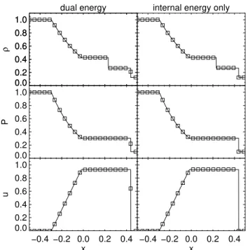
1.1 Summary of short-lived radioisotopes in the early solar system. . . 2
3.1 Turbulence model constants . . . 25
3.2 Mixing layer growth rates for Mc = 0.10. . . 31
4.1 Enrichment model parameters. . . 73
4.2 Summary of supernova-cloud interaction simulations and results. . . 93
LIST OF ABBREVIATIONS
AMR Adaptive mesh refinement
CAI Calcium-aluminum-rich inclusion CTU Corner transport upwind (method) ESS Early solar system
ILES Implicit large-eddy simulation IRDC Infrared dark cloud
ISM Interstellar medium
KH Kelvin-Helmholtz (instability) LES Large-eddy simulation
MHD Magnetohydrodynamics
OPR Ortho-to-para ratio
RANS Reynold-Averaged Navier-Stokes RM Richtmeyer-Meshkov (instability) RT Rayleigh-Taylor (instability) SLR Short-lived radioisotope SMR Static mesh refinement
SN Supernova
SNe Supernovae
SNR Supernova remnant
ST Sedov-Taylor
TILES Turbulent implicit large-eddy simulation
CHAPTER 1: INTRODUCTION
1.1 Short-lived radioisotopes
The solar system formed from the gravitational collapse of an interstellar gas cloud over 4.5 Gyr ago (Amelin et al., 2010). The gas cloud has long since dissipated, but a record of its physical conditions and chemical composition is preserved in meteorites. Calcium– aluminium-rich inclusions (CAIs) in chondritic meteorites are the oldest known solar system solids, with ages of≈ 4.567 Gyr (Amelin et al., 2002, 2010). Spectroscopic analyses of CAIs in the 1970s revealed isotopic excesses due to the in situ decay of short-lived radioisotopes (SLRs) (Lee et al., 1976, 1977), so named because of their half-lifetimes of . a few Myr (Russell et al., 2001; McKeegan & Davis, 2007). Table 1.1 summarizes the SLRs present in the early solar system (ESS) and their relative abundances inferred from meteoritic studies. The importance of these SLRs in solar system evolution lies in their radioactive nature. The SLRs present in the ESS were incorporated into small rocky bodies (planetesimals) and eventually planets, where their radioactive decay produced large amounts of heat. In particular, the decay of Aluminum-26 (denoted 26Al, τ
1/2 ≈ 0.7 Myr) and Iron-601 (τ1/2 ≈
2.6 Myr) fueled the differentiation of planetesimals (Sahijpal et al., 2007) and the internal melting of ice in rocky bodies (Travis & Schubert, 2005) during the first 10 Myr of solar system evolution (Urey, 1955). The sustained aqueous state in these bodies due to SLR heating may have allowed the synthesis of amino acids – the biomolecular precursors for life (Cobb & Pudritz, 2014). Understanding the origin of SLRs is therefore critical in assessing other planetary systems and the probability of life elsewhere in the cosmos.
1The number indicates the atomic mass; for these elements, the most common stable isotopes are
Table 1.1: Summary of short-lived radioisotopes in the early solar system. Parent τ1/2 Daughter Reference Initial Initial ESS
SLR (Myr) Isotope Isotope Abundance Ratio Mass Fraction
10Be 1.5 10B 9Be 3−10×10−4 6.5−22×10−14
26Al 0.72 26Mg 27Al 5.2×10⁻⁵ 3.3×10⁻⁹
36Cl 0.3 36Ar 35Cl &1.7×10⁻⁵ 9.4×10⁻¹¹
41Ca 0.1 41K 40Ca 4−6×10⁻⁹ 3.0−4.5×10⁻¹³
53Mn 3.7 53Cr 55Mn 6−8×10⁻⁶ 8.5−1.1×10⁻¹⁰
60Fe 2.6 60Ni 56Fe 3−7×10
−7 4.4−10×10−10
.7−12×10−9 1.0−1.8×10⁻¹¹
107Pd 6.5 107Ag 108Pd 5.9×10⁻⁵ 2.6×10⁻¹³
182Hf 8.9 182W 180Hf 1×10⁻⁴ 9.0×10⁻¹⁴
References: 10Be: McKeegan et al. (2000); Srinivasan & Chaussidon (2013); 26Al: Lee et al.
(1976); Jacobsen et al. (2008);36Cl: Lin et al. (2005); Jacobsen et al. (2009); 41Ca: Liu
et al. (2012); Srinivasan & Chaussidon (2013); 53Mn: Shukolyukov & Lugmair (2006); Trinquier et al. (2008);60Fe: Tachibana & Huss (2003); Mishra & Goswami (2014);
Moynier et al. (2011); Tang & Dauphas (2012); 107Pd: Chen & Wasserburg (1996);
Sch¨onb¨achler et al. (2008); 182Hf: Burkhardt et al. (2008); Kruijer et al. (2014). Initial ESS mass fraction is estimated using the initial solar abundances of Lodders (2003).
Measurements of the60Fe initial abundance based on secondary ionization mass
spectrometry (SIMS) and multi-collector inductively coupled plasma mass spectrometry (MC-ICPMS) do not agree; each is therefore reported independently.
The presence and abundance of SLRs also provides clues about the birth environment of the solar system. The presence of “live” SLRs in the ESS seems remarkable; SLRs rapidly decay and must therefore either be produced locally or quickly transported through the interstellar medium (ISM) from a nearby massive, evolved nucleosynthetic source (Lee et al., 1977). In the latter case, the presence of a nearby massive star provides constraints on the birth environment of the solar system, such as cluster size (Adams, 2010) and dynamical evolution (Parker et al., 2013; Pfalzner, 2013). However, the conditions leading to enrichment are uncertain. The initial abundances of some SLRs in the ESS appear to be enhanced above the Galactic background level (Diehl et al., 2006), but similar conditions may be common in star-forming regions (Vasileiadis et al., 2013; Jura et al., 2013; Young, 2014).
can produce some SLRs (e.g. 10Be) but not all (e.g. 60Fe) (Heymann & Dziczkaniec, 1976; Gounelle & Meibom, 2008). Although recent estimates of the initial 60Fe/56Fe ratio argue against significant 60Fe enrichment (Tang & Dauphas, 2012), the enhanced 26Al/27Al ratio
probably requires external sources (Makide et al., 2013). Asymptotic giant branch (AGB) star winds (Wasserburg et al., 1994), Wolf–Rayet (WR) winds (Prantzos & Casse, 1986), or Type II (core-collapse) supernova (SN) shock waves (Cameron & Truran, 1977) could transport SLRs and contaminate the ESS at some phase of its evolution (e.g. pre-solar molecular cloud, pre-stellar core, or proto-planetary disc).
1.1.1 Supernova enrichment
Among the various enrichment sources, Type II supernovae (SNe) have received the most attention in the literature (Cameron & Truran, 1977; Foster & Boss, 1997; Ouellette et al., 2005; Pan et al., 2012). SNe are naturally associated with star-forming regions, and predicted SLR yields from SNe match reasonably well with ESS abundance estimates (Meyer & Clayton, 2000). Additional evidence is provided by the anomalous ratio of oxygen isotopes ([18O]/[17O]) in the solar system, which is best explained by enrichment from Type II SNe
(Young et al., 2011).
Following the discovery of 26Al in CAIs, Cameron & Truran (1977) suggested that a
and choreography. The SN must be close to the pre-stellar core (. 0.1–4 pc) at the time of explosion to prevent significant SLR radioactive decay during transit; yet the SN shock must slow considerably (from & 2000 km s−1 at ejection to . 70 km s−1 at impact) to prevent
destruction of the core, requiring either large separation (&10 pc) or very dense intervening gas (&100 cm−3). Gritschneder et al. (2012) demonstrated that injection at higher velocities
(up to 270 km s−1) may be possible, but this is yet to be confirmed in three-dimensional
models.
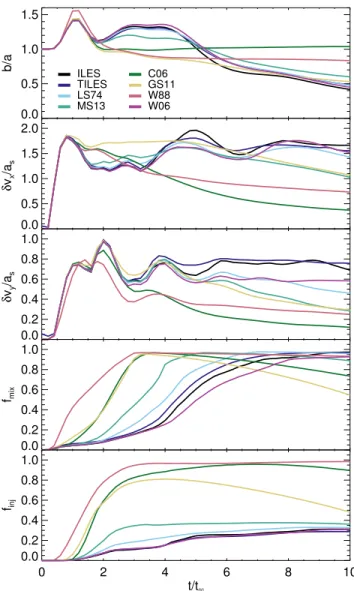
The amount of SLRs injected in the ‘triggered formation’ scenario is typically below observed values; both Boss & Keiser (2014) and Gritschneder et al. (2012) find SLR injection efficiencies . 0.01, compatible with only the lowest estimates for ESS values (Takigawa et al., 2008). Enrichment relies on hydrodynamical mixing of the ejecta into the pre-stellar gas, primarily via the Rayleigh–Taylor (RT) instability (Boss & Keiser, 2012). However, mixing in inviscid hydrodynamical simulations is controlled by numerical viscosity; because the instabilities grow fastest on the smallest scales, the details of the small-scale mixing are dominated by resolution effects. Shin et al. (2008) found that all quantities except the mixing fraction show convergence in shock-cloud simulations, similar to those performed by Boss & Keiser (2014). Hence estimates of the SLR injection from hydrodynamical simulations may be underestimated due to numerical effects.
1.1.2 Models for turbulent mixing
enrichment, as the environments and physics are different in each application.
I therefore develop a common framework for two-equation Reynolds-Averaged Navier-Stokes (RANS) turbulence models (Goodson et al., 2017), and I implement six such models in theAthenahydrodynamics code (Stone et al., 2008). I verify each implementation with
the standard subsonic mixing layer, although the level of agreement depends on the definition of the mixing layer width. I then test the validity of each model into the supersonic regime, showing that compressibility corrections can improve agreement with experiment. For models with buoyancy effects, I also verify the implementation via the growth of the Rayleigh-Taylor instability in a stratified medium. The models are then applied to the shock-cloud interaction in three dimensions. I focus on the mixing of shock and cloud material, comparing results from turbulence models to high-resolution simulations (up to 200 cells per cloud radius) and ensemble-averaged simulations. I find that the turbulence models lead to increased spreading and mixing of the cloud, although no two models predict the same result. Increased mixing is also observed in inviscid simulations at resolutions greater than 100 cells per radius; this suggests that the turbulent mixing only begins to be resolved at point and previous studies may underestimate the SLR injection.
1.1.3 Supernova dust grains
Even with a turbulence model, hydrodynamical mixing alone may not be sufficient to explain the enrichment of the ESS. The (linear) growth rates of the involved fluid instabilities depend on the square root of the density contrast (Chandrasekhar, 1961), resulting in an inevitable impedance mismatch between the hot, diffuse stellar ejecta and the cold, dense pre-solar core.
dense cloud, and gas-phase SLR injection occurs slowly due to hydrodynamical instabilities at the cloud surface. In contrast, dust grains of sufficient size (& 1 µm) decouple from the gas and rapidly penetrate into the cloud. Once inside the cloud, the dust grains are destroyed, releasing SLRs and rapidly enriching the dense (potentially star-forming) regions. This suggests that SLR transport on dust grains is a viable mechanism to explain SLR enrichment. Furthermore, dust grains of different sizes penetrate different distances, which could explain the discrepancy between 26Al and 60Fe in CAIs.
1.1.4 Massive star formation timescales
As indicated above, the primary source of SLRs is massive, evolved stars (>8M). A key
constraint on models of supernova enrichment is the timescale for massive star formation (Gounelle et al., 2009; Gaidos et al., 2009). Since the SLRs rapidly decay, the SN must be close to the ESS in both time and distance, preferably within the same molecular cloud complex. Since the age spreads of clusters are small (Hartmann et al., 2001; Hartmann, 2003), enrichment is most likely if the SN progenitor forms first and forms rapidly. Yet it is unclear from dynamical observations whether massive stars form slowly (Tan et al., 2013) or rapidly (V´azquez-Semadeni et al., 2007). An alternative means to probe the age and state of massive starless cores is using chemical tracers, in particular deuterated molecules (Ceccarelli et al., 2014). In sufficiently dense (nH>105 cm−3), cold (T <20 K) environments, CO freeze-out
opens a pathway for ion-neutral reactions that increase the deuterium fraction, i.e., the ratio of deuterated to non-deuterated species, Dfrac. High levels of deuterium fraction in N2H+
are observed in some pre-stellar cores (Kong et al., 2016). Single-zone chemical models find that the timescale required to reach observed values (DN2Hfrac+ ≡N2D+/N2H+ &0.1) is longer
than the free-fall time, possibly ten times longer (Kong et al., 2015).
of the core using each tracer for comparison to observations (Kong et al., 2017). I find that the velocity dispersion of the core as traced by N2D+ appears slightly sub-virial compared
to predictions of the Turbulent Core Model of McKee & Tan (2003), except at late times just before the onset of protostar formation. By varying the initial mass surface density, the magnetic energy, the chemical age, and the ortho-to-para ratio of H2, I also determine
the physical and temporal properties required for high deuteration. I find that low initial ortho-to-para ratios (.0.01) and/or multiple free-fall times (&3) of prior chemical evolution are necessary to reach the observed values of deuterium fraction in pre-stellar cores. This suggests that the collapse rate may be significantly slower than the free-fall time, or the deuteration process begins earlier than assumed.
1.2 Overview of contents
Chapter 2 provides an overview of the Athena magnetohydrodynamics code, as well
CHAPTER 2: NUMERICAL METHODS
2.1 The Athena code
The evolution of an ideal, inviscid magnetized fluid is governed by three conservation equations for the mass, the momentum, and the energy:
∂ρ
∂t +∇ ·(ρu) = 0 (2.1.1)
∂ρu
∂t +∇ ·(ρuu−BB+
B·B
2 +PI) = 0 (2.1.2)
∂E
∂t +∇ ·[(E+P + B·B
2 )u] = 0 (2.1.3)
with the density ρ, the velocity vector u, the magnetic field vector B1, the unit dyad I, the
thermal pressure P, and the total energy densityE:
E = P
γ−1+
1 2ρ|u|
2
+B·B
2 , (2.1.4)
where the ideal gas law P = (γ−1)e has been used to relate the pressure P to the internal energy density e via the adiabatic index γ. For magnetized fluids, Maxwell’s relations must be coupled with the fluid equations. For an ideal (perfectly-conducting) plasma, Faraday’s law and Ohm’s law lead to the induction equation:
∂B
∂t − ∇ ×(u×B) = 0. (2.1.5)
Finally, in many applications it is helpful to evolve a passive color field:
∂ρC
∂t +∇ ·(ρuC) = 0. (2.1.6)
Color fields do not affect the dynamics; they are therefore often used to trace the flow and mixing of different fluids or to follow chemical abundances.
We use theAthenamagnetohydrodynamics (MHD) code (Stone et al., 2008) to numer-ically solve Eqs. 2.1.1-2.1.6. Athena integrates the fluid equations using a finite-volume method on a uniform Cartesian grid in three dimensions. The hydrodynamical variables (ρ,
u,E) are represented as volume-averages at cell centers, while the magnetic fields (B) are rep-resented as an area-average at cell interfaces. Athenauses a high-order Godunov method;
in short, the time integration is performed by computing time- and area-averaged fluxes at cell interfaces as a solution to the Riemann problem. The Riemann problem describes the one-dimensional evolution of two uniform gases initially separated by an interface. If the gas properties are discontinuous across the interface, removal of the interface will generate a family of waves that propagate through the fluids with characteristic speeds dependent on the initial conditions. The Godunov method treats the evolution of fluids through each cell interface at each time step as a Riemann initial value problem. Further details of the Riemann problem and its extension to three-dimensions are given by Toro (2009).
The Godunov method used in Athena has three main elements: the time integration
scheme, the spatial reconstruction scheme, and the Riemann solver. Two directionally-unsplit integration methods are available: the corner transport upwind method (CTU) of Colella (1990) and the predictor-corrector method of van Leer (2006) (VL; see also Stone & Gardiner, 2009). Both methods employ constrained transport (CT; Evans & Hawley, 1988) to preserve the divergence–free constraint on the magnetic field. Athena uses the spatial
solutions are often used. We prefer solvers in the HLL family (Harten et al., 1983) that average over intermediate states in the Riemann problem. For hydrodynamics, we use the HLLC solver (Toro, 2009) which includes the contact wave; this is extended for MHD to include the Alfv´en wave in the HLLD solver (Miyoshi & Kusano, 2005).
Athena conserves the mass, momentum, total energy, and divergence of the magnetic
field to machine accuracy. Eqs. 2.1.1-2.1.6 do not include viscosity; however, the discretiza-tion, integradiscretiza-tion, and interpolation introduce numerical viscosity proportional to the grid resolution, time accuracy, and interpolation order, respectively. This allows Athena to
handle non-conservative phenomena such as supersonic shocks. Eqs. 2.1.1-2.1.3 also do not include additional source terms such as gravity and radiative cooling. Gravity is implemented in Athena in a way that conserves momentum but not energy (see Section 2.2.2). Other sources, such as diffusion and radiative cooling, are implemented at first order in time via operator splitting.
2.2 Modifications to Athena
2.2.1 Dual energy formulation
Certain source terms, such as radiative cooling, require the temperature T, which is proportional to the internal energy density e = P/(γ −1) via the ideal gas law. Athena
evolves the total energy density E, and the internal energy is evaluated by subtracting the kinetic energy Ekin ≡ρ|u|2/2 from the total energy. In regions where the kinetic energy is a
significant fraction of the total energy, the difference will be susceptible to numerical errors and the internal energy returned may be non-physical (e <0). Therefore, we simultaneously solve the internal energy equation:
∂e
If the internal energy is a small fraction of the total energy (e/E ≤10−3), we revert to using
erather than E−Ekin. This “Dual Energy Formulation” is also used inEnzo(Bryan et al.,
2014) andFlash (Fryxell et al., 2000). The check is performed any time the internal energy (or pressure or temperature) is required, such as calculating the pressure at cell interfaces as inputs to the Riemann solver. We prefer the dual energy formulation over a pressure or temperature floor in our models; while reverting the pressure to a small number (∼ 10−20)
may not affect the dynamics in most situations, the cooling depends very sensitively on the temperature.
The internal energy equation (Eq. 2.2.1) is not conservative. The left-hand side can be treated as an advection equation for e/ρ. We therefore use the density flux returned from the Riemann solver to advect the internal energy, treating e as a passive color field. The source term is calculated and applied at cell centers using a monotonic central difference to evaluate the gradients of the velocity in each direction. In contrast to Bryan et al. (2014), we use the updated pressure [calculated from P =e(γ−1)] when applying the source term at the full time-step update in the integrator. The non-conservative formulation can lead to large discrepancies from the correct internal energy if the equation is allowed to evolve on its own (see Figure 2.1). Therefore, we follow the recommendation of Bryan et al. (2014) and synchronize the internal energy using the total energy when deemed safe to do so. We reset e= (E−ρ|u|2/2) ife/E
max ≥0.1, where Emaxis the maximum total energy of the cell
and its immediate neighbours [eq. 45 of Bryan et al. (2014) with η2 = 0.1].
Test case: Sod shock tube
0.0 0.2 0.4 0.6 0.8 1.0
0.0 0.2 0.4 0.6 0.8 1.0
ρ
dual energy
0.0 0.2 0.4 0.6 0.8 1.0
P
−0.4 −0.2 0.0 0.2 0.4 x
0.0 0.2 0.4 0.6 0.8 1.0
u
internal energy only
−0.4 −0.2 0.0 0.2 0.4 x
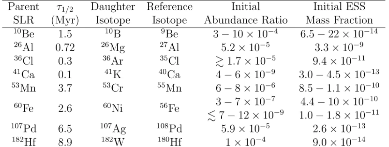
Figure 2.1: Profiles of the density, pressure, and velocity in the 1D Sod shock tube test case with 1024 grid points at t = 0.25 (in computational units). The analytic solution is shown as the solid line, with simulation results overplotted in open squares. From left to right in each profile are the rarefaction, contact, and shock discontinuities. The left column shows the result obtained with the standard dual energy method, while the right column shows the result when only the internal energy is used. The results show good agreement except in the shock front, which proceeds too slowly if only the internal energy is used.
wave. We test the dual energy formulation in two ways: 1) as described above with checks and syncing of the total energy, and 2) completely using the internal energy instead of the total energy. The latter represents the worst-case scenario; in practice, the internal energy is a fall-back mechanism only used in a neglible fraction of cells per time-step.
Figure 2.1 shows the density, pressure, and velocity in the Sod shock tube at t = 0.25 (in computational units). The left column shows the standard dual energy formulation, while the right column shows the worst-case scenario. In the standard case, the dual energy shows excellent agreement with the analytic solution; the rms error on the energy is 7.04×
10−4. However, if only the internal energy is evolved (and not the total energy), the shock
propagates too slowly and the rms error on the energy increases to 5.26×10⁻³. This illustrates
method used in calculating the velocity gradients. Despite this, the internal energy is still very accurate in the rarefaction and contact regions. As previously mentioned, the internal energy is only rarely used as a fallback mechanism. Overall, the dual energy formulation maintains a high degree of accuracy while preventing unphysical states and avoiding ad hoc
floor values.
2.2.2 Gravity
Gravity is implemented inAthenain a way that conserves momentum but not energy:
∂ρu
∂t +∇ ·(ρuu−BB+
B·B
2 +PI+Tg) = 0 (2.2.2)
∂E
∂t +∇ ·[(E+P + B·B
2 )u] = −ρu· ∇φ (2.2.3)
where φ is the gravitational potential and Tg is the gravitational tensor defined as (Jiang
et al., 2013):
Tg =
1
4πG[∇φ∇φ−
1
2(∇φ)·(∇φ)I] (2.2.4) with G the gravitational constant. This allows the momentum change due to gravity to be treated as a flux rather than a source term. The potential φ is evaluated at each time step via solution of Poisson’s equation,
∇2φ = 4πGρ. (2.2.5)
This elliptic partial differential equation can be evaluated using a variety of methods, such as multigrid methods or Fourier transforms, provided an approriate discretization and boundary conditions.
2.2.3 Gravity with SMR
Athena includes static mesh refinement (SMR) which allows for additional grid
grids remain in a fixed location for the duration of the simulation. This provides strict con-trol over where and how refinement is achieved. Unfortunately, mesh refinement complicates standard solving procedures for gravity. Athena currently does not support gravity with SMR. We have thererfore implemented a new gravitational potential solver compatible with SMR.
We follow a procedure similar to that used in Enzo (Bryan et al., 2014). We use
an iterative process to determine the gravitational potential level-by-level. First, we use a standard FFT-based method to compute the potential on the root domain, for either isolated or periodic boundary conditions. We then prolongate (interpolate) the potential to set boundary conditions on the next finer level. These values are used as Dirichlet boundary conditions for a Poisson solve on the fine domain. We use the standard second-order finite-difference approximation to the Poisson equation. The resulting linear equation is solved with the Hypre library (Falgout et al., 2006). Hypre provides easy access to a variety of
parallelized multigrid methods. The resulting potential is then interpolated to the next fine domain, and the process repeats. Finally, all fine domain potentials are restricted (averaged) back onto the coarse domains to reduce errors.
We use the same prolongation and restriction operators as Athena uses for the scalar hydrodynamic variables, namely those of T´oth & Roe (2002). For prolongation, this is a conservative linear interpolation with a monotonic slope limiter. The slope limiter prevents new extrema as a result of interpolation. Athena prolongates a single cell-centered coarse
value into a 2×2×2 (in 3D) cube of fine-grid values. The method is conservative in that the mean of the cube of values is equivalent to the coarse value. However, the linear interpolation routine is slightly inaccurate for fields with non-linear gradients. As an example, consider a smooth point-mass potential going as r−1. The linear interpolation will overshoot on one
−1 0 1 x
−1 0 1
y
−3.5 −3.0 −2.5 −2.0 −1.5 −1.0 −0.5
potential
−1 0 1
x −1
0 1
y
−5.0 −4.5 −4.0 −3.5 −3.0 −2.5
log relative error
Figure 2.2: Midplane slice at z = 0 of the gravitational potential (left panel) resulting from an oblate spheroid determined using Hypre on a single fixed grid of 1283 cells. The log
of the relative error is also shown (right panel). Hypre use parallelized multigrid methods
to solve the linear system resulting from the finite-difference approximation to the Poisson equation. Boundary conditions are evaluating using a high-order multipole expansion.
solve. The fine grid density field is not interpolated, and therefore the resulting potential is (overall) smooth.
Test case: MacLaurin spheroid
A homoegenous oblate spheroid (or so-called “MacLaurin” spheroid) is ideal for testing the accuracy of gravity solvers (Couch et al., 2013) because the potential can be expressed analytically (Ricker, 2008) and the partial symmetry will reveal dimension-dependent errors. We initialize a static oblate spheroid with semi-major axis a = 1.0, ellipticity e = 0.9, and uniform density ρ= 1.0 in a negligible background ρ0 = 10−10. The spheroid is centered in
a simulation cube of width L= 4.0.
We first test our new Hypre-based Poisson solver on a single fixed grid of 1283 support
−1 0 1 x
−1 0 1
y
−3.5 −3.0 −2.5 −2.0 −1.5 −1.0 −0.5
potential
−1 0 1
x −1
0 1
y
−5.0 −4.5 −4.0 −3.5 −3.0 −2.5
log relative error
Figure 2.3: Same as Figure 2.2, but for a nested SMR grid of three levels. The root grid is 323, resulting in an effective resolution of 1283. The SMR refinement boxes are barely visible
in the error (right panel) due to the interpolation from coarse to fine levels.
boundaries. The solution to linear system resulting from discretization of Eq. 2.2.5 is evaluated using the generalized minimal residual (GMRES) method with a semicoarsening multigrid (SMG) pre-conditioner. Figure 2.2 shows the potential and relative error in a midplane slice at z = 0. Comparing to the analytic solution, our solver yields an rms relative error of 3.2×10⁻⁶, with a maximum error of 3.5×10⁻³.
We then test the solver on a nested SMR grid of three levels, with 323 support points on the coarest level and an effective resolution of 1283 on the finest level. Similar to Figure 2.2, Figure 2.3 shows the potential and relative error in a midplane slice at z = 0. The outlines of the SMR refinement grids are visible in the error, but overall the potential is still highly accurate. Compared to the fixed grid, the rms error and maximum error are only slightly increased to 4.0×10⁻⁶ and 4.5× 10⁻³, respectively. Most importantly, the use of SMR
2.2.4 Dust dynamics
Particles, such as dust grains, follow a different equation of motion which must be solved simultaneously. We have added passive particles to the VL integrator (Stone & Gardiner, 2009) in Athena(Stone et al., 2008). The particle update is performed using the predictor
values. Comparisons with the CTU integrator, which includes particles by default, show nearly absolute agreement. We have also extendedAthenato include drag forces, collisional
CHAPTER 3: TURBULENCE MODELS IN THE SHOCK-CLOUD
INTERACTION1
3.1 Introduction
Since the discovery of26Al in CAIs by Lee et al. (1976), the leading hypothesis has been
injection of SLRs by a nearby supernova (Cameron & Truran, 1977; Margolis, 1979). In this scenario, a SN launches a supersonic blast wave carrying SLRs into the ISM that collides with nearby molecular gas clouds (McKee & Ostriker, 1977). The impinging shock wave drives hydrodynamic instabilities at the cloud surface, such as the Rayleigh-Taylor (RT), Kelvin-Helmholtz (KH), and Richtmeyer-Meshkov (RM) instabilities (Stone & Norman, 1992), that could simultaneously inject SLRs and trigger gravitational collapse (Foster & Boss, 1997).
If the blast wave has traveled sufficient distance, or if the target cloud is sufficiently small, the blast wave can be considered approximately planar when it collides with the molecular cloud. In this case, the interaction resembles the standard shock-cloud interaction – a well-studied problem in numerical simulations (Stone & Norman, 1992; Klein et al., 1994; Xu & Stone, 1995; Nakamura et al., 2006; Pittard et al., 2009; Pittard & Parkin, 2016). Foster & Boss (1997) first performed shock-cloud simulations of SN enrichment, and subsequent shock-cloud experiments (Boss et al., 2010; Boss & Keiser, 2012, 2013, 2014, 2015) have extending the physics and parameter space. Yet these simulations encounter a common bottleneck – it remains difficult to mix the hot SN ejecta into the dense molecular cloud without disrupting the cloud. Most recently, Boss & Keiser (2015) find that less than
1Portions of this chapter previously appeared as an article in Monthly Notices of the Royal Astronomical
10% of incident SN material is injected into a dense pre-solar core, reaching only the lowest estimates for ESS abundances (Takigawa et al., 2008).
It may be that the mixing observed in shock-cloud simulations is artificially suppressed by insufficient resolution. In Goodson et al. (2017), we explore the dynamics and mixing of the shock-cloud interaction in detail. We consider turbulence models as a means to reduce resolution effects, and we implement six models in the Athena code. We test the ability
of the models to capture hydrodynamical instabilities, and we apply the models to a shock-cloud interaction in three dimensions. We find that the turbulence models predict higher levels of mixing, with injection fractions & 30%. Increased mixing is also seen in inviscid simulations only once sufficient resolution is achieved (greater than 50 cells per cloud radius). This suggests that the turbulent cascade begins to be resolved at this point, and simulations with lower resolutions may underestimate the turbulent mixing.
3.1.1 Hydrodynamical modeling of the shock-cloud interaction
In Eulerian hydrodynamics simulations, the growth of turbulence is controlled by nu-merical viscosity (resolution effects). Adequate resolution is therefore necessary to properly capture the dynamics. Previous work on the shock-cloud interaction has found that about 100 cells per radius are necessary for convergence of global quantities (Klein et al., 1994; Nakamura et al., 2006; Pittard et al., 2009), although this requirement may be relaxed in 3D simulations (Pittard & Parkin, 2016). However, because the instabilities grow fastest on the smallest scales, the details of the small-scale mixing are dominated by resolution effects. Shin et al. (2008, hereafter SSS08) found that all quantities except the mixing fraction show convergence in shock-cloud simulations.
used in astrophysics (Schmidt et al., 2006; Scannapieco & Br¨uggen, 2008; Pittard et al., 2009; Gray & Scannapieco, 2011; Schmidt & Federrath, 2011; Schmidt, 2014; Pittard & Parkin, 2016). Turbulence models can be separated into two types: Reynolds-averaged Navier-Stokes (RANS) and Large-Eddy Simulations (LES). The former relies on time-averaging of the de-composed fluid equations, while the latter uses spatial filtering of variables. Here, we only consider RANS models; for a review of LES methods, see Schmidt (2014).
3.1.2 Turbulence models in the shock-cloud interaction
Both RANS and LES turbulence models have been used to model the interaction of a shock with a cloud, in different environments and with different results. Pittard et al. (2009, hereafter P09) examined the hydrodynamic shock-cloud interaction in two dimensions with the k-ε model, a two-equation RANS model. The authors argued that the k-ε turbulence model adequately captured the dynamics of the shock-cloud interaction and reduced the resolution requirements. Follow-up studies by Pittard & Parkin (2016, hereafter PP16) revealed that thek-εmodel did not significantly alter the dynamics or improve the resolution convergence in three dimensional simulations.
Gray & Scannapieco (2011, hereafter GS11) used a different two-equation RANS model, based on thek-Lformalism, to track metal enrichment in so-called “minihalos”. An enriched supersonic galactic outflow impacts a diffuse cloud of primordial gas, subject to both gravity and radiative cooling. The authors modified the k-L model of Dimonte & Tipton (2006, hereafter DT06), which was calibrated for RT and RM instabilities, to include the KH in-stability and compressibility effects. Here the authors specifically investigated the turbulent mixing of metals. While there were notable differences in the enrichment of diffuse gas, the metal abundance in the dense gas was largely unaffected by the turbulence model.
For this application, the authors used a linear eddy-viscosity relation with a dynamic proce-dure to calculate transport coefficients (“shear-improved” SGS model). The authors found that, while the LES turbulence model did not significantly alter the energy of the interaction, it did affect the vorticity and subsequent evolution of the infalling gas.
It is difficult to interpret and compare the effects of the turbulence models in the sim-ulations described above. First, each application explored different physical regimes and therefore included different physics (e.g. radiative cooling, gravity). Second, some turbu-lence models incorporated additional effects, such as buoyancy and compressibility, that other models implicitly neglect. Third, each turbulence model affects the dynamics differ-ently. In the case of LES, the resolved dynamics are largely unaffected, as the model only considers turbulent effects near and below the filter width, which is typically close to the grid scale. However, RANS models average out dynamical fluctuations at all scales below some characteristic length scale, which varies throughout the simulation and could be much larger than the grid scale. Fourth, the “true” solution to the shock-cloud interaction is unknown. One can compare results obtained with a turbulence model to higher-resolution simulations, but without an explicit viscosity the degree of mixing remains constrained by the numerical viscosity.
3.1.3 Motivation and outline
In an effort to better understand the effects and validity of turbulence models in astro-physical applications such as SLR enrichment, we perform hydrodynamical simulations of the generic shock-cloud interaction with six two-equation RANS models. We first develop a common framework for two-equation turbulence models, and we implement this framework in the Athena hydrodynamics code (Stone et al., 2008). We verify the implementation of
each turbulence model with the subsonic shear mixing layer test, ensuring that the width of the mixing layer grows linearly in accord with experimental results. We also highlight the dependence of the growth rate on the definition of the mixing layer width. We then test the validity of each model into the supersonic regime. Most models are known to perform poorly in transonic applications, but we explore three common “compressibility corrections” that improve results. Three of the models here considered include buoyancy effects, such as the RT instability. For these models, we further verify our implementation with a strat-ified medium test, in which we compare the temporal growth of the RT boundary layer to experimental results.
After determining that the turbulence models are implemented correctly, we test each turbulence model in a three-dimensional adiabatic shock-cloud interaction. We quantify not only the global dynamics but also the small-scale mixing. To examine the validity of the turbulence models, we perform a resolution convergence test of the inviscid shock-cloud interaction, up to 200 cells per radius in full 3D on a fixed grid. We also compare results to an ensemble-average of inviscid simulations initialized with grid-scale initial turbulence, scaled to roughly match the initial conditions of the turbulence models. Finally, we consider the effects of initial conditions and compressibility corrections in the turbulence models, finding that the former makes a significant difference in evolution whereas the latter does not.
We outline the six RANS turbulence models and their implementation in Athena in
turbulence models are then used in the shock-cloud simulation; the set-up and results of these simulations are presented and discussed in Section 3.5. Finally, we discuss the validity of turbulence models in astrophysical applications in Section 3.6 before concluding in Section 3.7.
3.2 Turbulence models
We extend Eqs. 2.1.1 – 2.1.6 as follows:2
∂ρ
∂t +∇ ·(ρu) = 0 (3.2.1)
∂(ρu)
∂t +∇ ·(ρuu+PI) = ∇ ·τ 0
(3.2.2)
∂E
∂t +∇ ·[(E+P)u] =∇ ·(uτ 0 −
q0) + ΨE (3.2.3)
∂(ρC)
∂t +∇ ·(ρCu) = ∇ ·d
0
(3.2.4)
∂(ρk)
∂t +∇ ·(ρku) = ∇ ·( µT
σk
∇k) + Ψk (3.2.5)
∂(ρξ)
∂t +∇ ·(ρξu) = ∇ ·( µT
σξ
∇ξ) + Ψξ (3.2.6)
with the specific turbulent kinetic energyk, an auxiliary turbulence variableξ, the turbulent stress tensorτ0, the turbulent heat flux q0, the turbulent diffusive flux d0, turbulent viscosity
µT, turbulent diffusion coefficients σ, and source terms due to turbulent effects Ψ. E now represents the total resolved energy density E 3.
Two-equation models are so named because they add two “turbulent” variables – the specific turbulent kinetic energy k and an auxiliary variable ξ that varies from model to model – with corresponding transport equations (Eqs. 3.2.5-3.2.6). Models are typically
2For simplicity of notation, we do not differentiate Reynolds-averaged (ρ, P) and Favre-averaged (˜u,E,˜ C˜)
variables, where ˜φ≡ρφ/ρ.
3We do not include the turbulent kinetic energy ρk in the definition of total energy; therefore we are
denoted by the chosen auxiliary turbulence variable; e.g., ξ→ε yields thek-ε model. Here, we examine the standard k-ε model of Launder & Spalding (1974, hereafter LS74), as well as the extended model of Mor´an-L´opez & Schilling (2013, hereafter MS13); the k-L models of Chiravalle (2006, hereafter C06) and GS11; and thek-ω models of Wilcox (1988, hereafter W88) and Wilcox (2006, hereafter W06). For thek-εand k-ω models, we also test the effect of three standard compressibility corrections, presented in Sarkar et al. (1989, hereafter S89), Zeman (1990, hereafter Z90), and Wilcox (1992, hereafter W92).
The turbulent stress tensorτ0 is defined as
τij0 = 2µT(Sij− 1
3δijSkk)− 2
3δijρk (3.2.7)
with resolved stress rate tensorS given by
Sij = 1 2(
∂ui
∂xj
+∂uj
∂xi
). (3.2.8)
The specific turbulent kinetic energyk is defined as k ≡(1/2)τkk0 and requires an additional transport equation. The generic transport equation (Eq. 3.2.5) is applicable to (almost) all models investigated, with source term
Ψk=PT −CDρε+CBρ
√
kAigi (3.2.9)
with the production term PT = τij0 ∂ui/∂xj, specific dissipation ε, dissipation coefficient
CD, buoyancy coefficient CB, and Atwood number in the ith direction Ai with acceleration
gi = −(1/ρ)∂P/∂xi. The source term on the energy equation is ΨE = −Ψk. Table 3.1 presents a summary of all model constants and values.
In adiabatic simulations, the turbulent heat flux vectorq0 is defined as
q0j =−κT
∂T ∂xj
= γ
γ−1
µT
P rT
∂T ∂xj
Table 3.1: Summary of model constants. Some values may appear at variance with the reference; this is due only to our generic formalism, which redefines and combines certain constants for consistency across all models. Values presented for the W06 model neglect limiting functions and should therefore be considered approximations.
Constant Description LS74 MS13 C06 GS11 W88 W06
Cµ Turbulent viscosity 0.09 0.09 0.30 1.00 1.00 1.00
CD Dissipation of turbulence 1.00 1.00 8.91 3.54 0.09 0.09
CB Buoyancy effects 0.00 0.10 1.70 1.19 0.00 0.00
P rT Turbulent Prandtl number 0.90 0.90 1.00 1.00 0.90 0.89
σk Turbulent energy diffusion 1.00 0.50 1.00 1.00 2.00 1.67
σξ Turbulent diffusion 1.30 0.50 1.00 0.50 2.00 2.00
σC Turbulent Schmidt number 1.00 0.50 1.00 1.00 1.00 1.00
C1 Turbulence generation 1.44 1.44 1.00 0.33 0.56 0.52 C2 Additional effects 1.92 1.92 1.00 1.00 0.08 0.07
C3 Buoyancy effects 0.00 0.09 0.00 0.00 0.00 0.00
with turbulent thermal conductivity κT =cpµT/P rT, specific heat capacity cp =γ/(γ −1), and turbulent Prandtl number P rT.
Passively advected scalar fields are diffused using a gradient-diffusion approximation, where the turbulent diffusive flux vector d0 is given by
d0j = µT
σC
∂C ∂xj
, (3.2.11)
with Schmidt number σC generally of order unity.
3.2.1 k-ε models
In the k-ε formalism, the auxiliary turbulence variable ξ is defined to be the specific turbulent energy dissipation ε ∝k3/2L−1, where L is a defined turbulent length scale. The
LS74
LS74 outlined the standard version of the k-ε model, and it is perhaps the most widely used RANS turbulence model. The model uses the eddy-viscosity µT defined as
µT =Cµρ
k2
ε (3.2.12)
with Cµ= 0.09. The transport equation for ε (Eq. 3.2.6) has the source term
Ψε =C1ε
kPT −C2ρ ε2
k. (3.2.13)
The model constants are summarized in Table 3.1. Because CB = 0, the model neglects buoyant effects, such as the RT instability.
MS13
To include the RT and RM instability effects in thek-ε model, MS13 added a buoyancy term, with the Atwood number in Eq. 3.2.9 defined as
Ai =
k3/2 ρε (
∂ρ ∂xi
− ρ
P ∂P ∂xi
). (3.2.14)
The source term for the dissipation equation Ψε is also extended as
Ψε =C1 ε
kPT −C2ρ ε2
k +C3ρ ε √
kAigi. (3.2.15)
3.2.2 k-L models
Thek-Lmodel is a two-equation RANS model developed by DT06 to study RT and RM instabilities. Shear (KH instability) was added by C06 and extended to include compress-ibility effects by GS11. The auxiliary variable ξ is defined to be the eddy length scale L. The model uses the eddy-viscosity
µT =CµρL
√
2k. (3.2.16)
The transport equation for L (Eq. 3.2.6) has the source term
ΨL =C1ρL(∇ ·u) +C2ρ √
2k. (3.2.17)
Again, we here set the specific dissipation in Eq. 3.2.9 to beε =Cµ3/4k3/2L−1.
C06
C06 added shear to the k-L model of DT06 by employing the full stress tensor rather than just the turbulent pressure term. This necessitated re-calibrating the model coefficients of DT06. We note that C06 used a slightly different RT growth rate parameter (α = 0.05 instead of α = 0.0625 in DT06) when calibrating the model. Buoyancy effects are included via the Atwood number defined as
Ai =
ρ+−ρ− ρ++ρ−
+L
ρ ∂ρ ∂xi
, (3.2.18)
where ρ+ and ρ− are the reconstructed density values at the right and left cell faces,
GS11
Similar to C06, the model of GS11 is based on the k-L model of DT06, but with the complete turbulent stress tensor to include KH effects. The model uses a slightly different definition of the Atwood number from C06, with
Ai =
ρ+−ρ− ρ++ρ−
+ 2L
ρ+L|∂ρ/∂xi|
∂ρ ∂xi
, (3.2.19)
where again ρ+ and ρ− are the reconstructed density values at the right and left cell faces,
respectively.
GS11 also introduces a variable (τKH) to account for compressibility effects by modifying the turbulent stress tensor,
τij0 = 2µTτKH(Sij − 1
3δijSkk)− 2
3δijρk. (3.2.20)
τKH is calibrated with compressible shear layer simulations and estimated using a “local” Mach numberMl ≡ |∇ ×u|L/cs, where cs is the local sound speed. However, the piecewise fit forτKH given by Eq. 19 in GS11 is discontinuous, which can lead to numerical issues. We
therefore fit their formulation with a smooth function,
τKH(Ml) = 0.000575 +
0.19425
1.0 + 0.000337exp(17.791 Ml)
. (3.2.21)
The model constants are summarized in Table 3.1; we note that the C06 and GS11 model constants differ despite significant similarity in model formulation and calibration.
3.2.3 k-ω models
The k-ω model was first developed by W88 and updated in Wilcox (1998) and W06. The auxiliary variable ξ is defined to be the specific dissipation rate (or eddy frequency)
ω =k1/2L−1, which has units of inverse time. Then the specific dissipation isε=C
our knowledge, this is the first use of a k-ω model in an astrophysical application.
W88
The first version of thek-ωmodel is outlined in W88. The model uses the eddy-viscosity
µT =Cµ
ρk
ω . (3.2.22)
The transport equation for ω (Eq. 3.2.6) uses the source term
Ψω =C1 ω
kPT −C2ρω 2
. (3.2.23)
The model constants are summarized in Table 3.1.
W06
The most recent version of thek-ωmodel is presented in W06 and Wilcox (2008). While the model is similar to W88, there are important (and elaborate) differences, such as cross-diffusion terms and stress limiters. While the additional terms improve the accuracy and reduce the dependence on initial conditions, the model is sufficiently complex to prohibit a generic description. Our implementation in Athena includes the additional terms, and
we refer the reader to W06 and Wilcox (2008) for a full description of the model. For completeness we note approximate constant values in Table 3.1.
3.2.4 Compressibility corrections
turbulent Mach number Mt ≡
√
2k/as, with as the local sound speed. No further changes are needed in the k- formalism. In the k-ω formalism, Eq. 3.2.23 is also modified with
C2ρω2 → [C2 −CDF(Mt)]ρω2. We consider three forms for F(Mt) proposed in the litera-ture. The simplest model is that of S89 which uses
F(Mt) =Mt2. (3.2.24)
The most complex model is that of Z90 with
F(Mt) = 0.75{1.0−exp[−1.39(γ+ 1.0)(Mt−Mt0)2]}H(Mt−Mt0), (3.2.25)
with H the Heaviside step function and Mt0 ≡0.10 p
2/(γ+ 1). Finally, the model of W92 suggests
F(Mt) = 1.5(Mt2−0.0625)H(Mt−0.25). (3.2.26)
It is worth noting that these are purely phenomenological models; resolved DNS simulations by (Vreman et al., 1996) have demonstrated that the dissipation is not actually reduced in compressible turbulence. Despite this realization, compressibility corrections that modify the dissipation are still commonly used because they yield accurate results in many applications. As noted in Section 3.2.2, GS11 uses a different type of compressibility correction which modifies the turbulent stress tensor. No satisfactory correction is available for C06.
3.2.5 Turbulence model initial conditions
In simulations with a turbulence model, we must specify initial conditions for the tur-bulent kinetic energy k and the additional turbulent variable (ξ → ε, L, or ω). We desire identical initial conditions for all models; we therefore set the turbulent length scaleLin all models and convert using scaling relations. Based on dimensional arguments, ε ∝ k3/2/L
Table 3.2: Mixing layer growth rates for Mc = 0.10.
Model Cb10 Cb1 Cs10 Cω Cθ
empirical 0.082-0.100 a 0.170-0.181b 0.058-0.084 a 0.081-0.091a,c 0.016-0.018d
LS74 0.070 0.092 0.056 0.083 0.015
MS13 0.067 0.091 0.053 0.077 0.014
C06 0.181 0.206 0.143 0.066 0.038
GS11 0.123 0.189 0.100 0.134 0.026
W88 0.052 0.062 0.041 0.040 0.011
W06 0.061 0.074 0.047 0.069 0.013
aBarone et al. (2006); bPapamoschou & Roshko (1988), with δ
viz ≈δb1;cBrown & Roshko
(1974);dPantano & Sarkar (2002).
the best agreement across models using ε0 =C 3/4
µ k03/2L−01 and ω0 =C −1/4
µ k10/2L−01.
3.2.6 Implementation in Athena
The turbulence update is first order in time and implemented via operator splitting. The fluxes are calculated at cell walls using a simple average to reconstruct quantities from cell-centered values. Spatial derivatives are computed using second order central differences. Source terms are evaluated after application of the viscous fluxes and are applied with an adaptive Runge-Kutta-Fehlberg integrator (RKF45). Stability of the explicit diffusion method is preserved by limiting the overall hydrodynamic time step based on the condition ∆t ≤ (∆2ρ)/(6µT), where ∆ is the minimum cell size. The dependence on ∆2 limits the feasibility of our implementation to low resolution simulations.
3.3 Mixing layer test
To verify the implementation of each turbulence model in Athena, we perform a
right states sets the convective Mach number, defined as (Papamoschou & Roshko, 1988)
Mc≡
|vl−vr|
cl+cr
, (3.3.1)
with v the y-velocity and c the sound speed, with subscripts l and r for the left and right regions respectively. Unlike GS11, we shift the frame of reference to move at the convective velocity; then vl =−vr. We also smooth the initial velocity discontinuity with a hyperbolic tangent function, as was done in Palotti et al. (2008). The parallel (x) velocity is zero. We use an ideal equation of state with γ = 1.4. The density and pressure are constant at
ρ0 = 1.0 g cm−3 and P0 = 1.72×10¹⁰erg cm−3, corresponding to a uniform sound speed cl=
cr= 1.55×105cm s−1. The simulation domain is a one-dimensional region with extent -5.0 cm
< x < 5.0 cm with a resolution of 4096 cells. Similar to GS11, we initialize a small shear layer of width δ0 = 0.1 cm centered at the interface with turbulent energy k = 0.02(∆v)2 and L = 0.2δ0, where ∆v =|vl−vr|. This initial layer is also smoothed to the background values of k0 = 10−4(∆v)2 and L0 = 10−2δ0.
We run each simulation for 200µs. The velocity discontinuity generates a shear layer, and the width of the shear layer δ grows linearly in time as
δ(t) =Cδ ∆v t, (3.3.2)
where Cδ is a constant. The exact value for Cδ depends on how the shear layer thickness δ is defined. In lab experiments, the visual thickness δviz (Brown & Roshko, 1974) or pressure
thicknessδp(Papamoschou & Roshko, 1988) are used. In numerical experiments, the velocity thickness δb, energy thickness δs, and vorticity thickness δω are often used (Barone et al., 2006); less common is the momentum thickness,δθ(Vreman et al., 1996). C06 and GS11 used a 1 per cent threshold on the velocity thickness (which we will denote as δb1), considering
(δs10), defined where 0.1<(v−vl)2/(∆v)2 <0.9. We will compare results using these three definitions, as well as the momentum thickness δθ = 1/[ρ0(∆v)2]
R
ρ(vl−v)(v−vr) dx and the vorticity thickness δω =|vl−vr|/(∂v/∂y)max.
A further complication is that lab experiments of the plane mixing layer measure a spatial spreading rate, δ0(x) ≡ dδ/dx. In our experiment, we move in a frame of reference at the convective velocity vc = (1/2)(vl+vr) (assuming cl = cr) and therefore measure a temporal spreading rate, (e.g., Vreman et al., 1996; Pantano & Sarkar, 2002)
δ0(t) = dδ
dt =
dx dt
dδ dx =vcδ
0
(x). (3.3.3)
Values for Cδ estimated from plane mixing layer experiments (Brown & Roshko, 1974; Pa-pamoschou & Roshko, 1988) and high-resolution numerical simulations (Pantano & Sarkar, 2002; Barone et al., 2006) are reported in Table 3.2, where the subscript on C indicates the corresponding shear layer thickness definition.
3.3.1 Mixing layer results
Figure 3.1 shows the time evolution of a subsonic (Mc = 0.1) mixing layer with the LS74 k-ε model. The profiles of the the y-velocity v, turbulent kinetic energy k, and turbulent length L all spread in time; as noted, the exact spreading rate depends on how the layer thickness is defined. Figure 3.2 shows the growth of the shear layer thicknessδ(t) for different layer definitions. All definitions show linear growth in time. The 1 per cent velocity thickness grows at the greatest rate, while the momentum thickness increases at the lowest rate. We use a χ2 minimization linear fit to estimate C
δ; the results are presented in Table 3.2. Table 3.2 also shows the growth rates atMc= 0.10 for all RANS models tested. We find
0 µs 50 µs 100 µs 200 µs −0.02 −0.01 0.00 0.01 0.02 v [cm µ s −1 ] 4 5 6 7
log k [cm
2 s −2]
−0.4 −0.2 0.0 0.2 0.4
x [cm] −3.0 −2.5 −2.0 −1.5 −1.0
log L [cm]
Figure 3.1: Time evolution of the one-dimensional subsonic (Mc = 0.10) shear flow test with
the LS74 k-ε turbulence model. From the top, profiles of the y-velocity v, specific turbulent kinetic energy k, and turbulent length scale L = Cµ3/4k3/2ε−1. Profiles are shown at times
t= 0, 50, 100, and 200 µs, indicated by colour.
0 50 100 150 200
0.0 0.2 0.4 0.6 0.8
0 50 100 150 200
t [µs] 0.0 0.2 0.4 0.6 0.8 δ [cm] velocity (10%) velocity (1%) energy (10%) vorticity momentum
Figure 3.2: Growth of the shear layer width δ(t) in the subsonic (Mc = 0.10) mixing layer
inAthena. Variations in numerical method between codes could lead to discrepancies with
previous work; further, there is significant uncertainty on the measured values. Interestingly, there is no clear relation between the different measures and models; for example, Cb10 is
much greater with the GS11 model compared to the LS74 model, but Cω is slightly less. This suggests no single measure should be preferred.
Finally, we note that C06 and GS11 calibrated their turbulence models using a 1 per cent velocity definition for the mixing layer. While their models show good agreement with this definition, we find that these models largely do not predict spreading rates in agreement with measured values when using other definitions. This suggests that a 1 per cent criterion may not be the best definition for comparison.
3.3.2 Compressible mixing layer
The spreading rate of a compressible mixing layer is found to decrease with increasing convective Mach number (Birch & Eggers, 1973; Brown & Roshko, 1974; Papamoschou & Roshko, 1988). The difference is expressed as the compressibility factor Φ≡δ0/δ0i, whereδ0iis the incompressible growth rate. Experiments have yielded different relations betweenMcand Φ, such as the popular “Langley” curve (Birch & Eggers, 1973), the results of Papamoschou & Roshko (1988), and the fit of Dimotakis (1991).
We perform simulations with increasing convective Mach number up toMc= 10. We use the growth rate determined atMc = 0.1 with thicknessδb10as our incompressible growth rate δ0i. Results obtained with the LS74 model are presented as solid circles in Figure 3.3, with two experimental curves shown for comparison. Although the spreading rate does decrease with increasing Mach number, it does not follow the experimental trend. This is consistent with previous work which shows that standard two-equation RANS turbulence models do not reproduce the observed reduction in spreading rate without modifications.
0.1 1.0 10.0 0.0
0.2 0.4 0.6 0.8 1.0
0.1 1.0 10.0
Mc 0.0
0.2 0.4 0.6 0.8 1.0
Φ
Dimotakis91 Barone+06
GS11 LS74+W92 LS74+Z90 LS74+S89 LS74
Figure 3.3: The compressibility factor Φ ≡ δ0/δi0 as a function of convective Mach number
Mc. Results are shown for the standard LS74 model with no compressibility correction (purple dots) and with the compressibility corrections of S89 (blue upward triangles), Z90 (green downward triangles), and W92 (gold diamonds); as well as for the GS11 model (red squares), which includes a stress modification (τKH). The empirical curves of Dimotakis (1991, dashed) and Barone et al. (2006, dot-dashed) are also shown for comparison.
the dissipation rate due to pressure-dilatation effects. Although direct numerical simulation results have shown that this is not actually the case (Vreman et al., 1996), these ad hoc
compressibility corrections are still widely used because they produce more accurate results (at least in the transonic regime). Figure 3.3 also shows results obtained when the three compressibility corrections are applied to the LS74 model. All three corrections do decrease the spreading rate to roughly the experimental values, at least up to Mc = 5; above this, the growth rate is slightly below the experimental estimate. The difference between the corrections of S89, Z90, and W92 is negligible. Similar results are obtained when applied to the MS13, W88, and W06 models.
There is no straightforward way to apply these corrections to the model of C06; however, GS11 does include a compressibility correction through the variableτKH (see Section 3.2.2).
Results obtained with the model of GS11 are also shown on Figure 3.3. The asymptotic nature of the τKH function (Eq. 3.2.21) reproduces the observed behavior of compressible