Autoencoder in Time-Series Analysis for
Unsupervised Tissue Characterisation in a Large
Unlabelled Medical Image Dataset
Hoo-Chang Shin, Matthew Orton, David J Collins, Simon Doran and Martin O Leach CRUK and EPSRC Cancer Imaging Centre
Institute of Cancer Research and Royal Marsden NHS Foundation Trust
Sutton, United Kingdom
Email:{hoo.shin, matthew.orton, david.collins, simon.doran, martin.leach}@icr.ac.uk
Abstract—The topic of deep-learning has recently received con-siderable attention in the machine learning research community, having great potential to liberate computer scientists from hand-engineering training datasets, because the method can learn the desired features automatically. This is particularly beneficial in medical research applications of machine learning, where getting good hand labelling of data is especially expensive.
We propose application of a single-layer sparse-autoencoder to dynamic contrast-enhanced magnetic resonance imaging (DCE-MRI) for fully automatic classification of tissue types in a large unlabelled dataset with minimal human interference – in a manner similar to data-mining. DCE-MRI analysis, looking at the change of the MR contrast-agent concentration over successively acquired images, is time-series analysis. We analyse the change of brightness (which is related to the contrast-agent concentration) of the DCE-MRI images over time to classify different tissue types in the images. Therefore our system is an application of an autoencoder to time-series analysis while the demonstrated result and further possible successive application areas are in computer vision.
We discuss the important factors affecting performance of the system in applying the autoencoder to the time-series analysis of DCE-MRI medical image data.
Index Terms—deep-learning, autoencoder, time-series analysis, medical image analysis, cancer, liver, DCE-MRI
I. INTRODUCTION
Automatic segmentation and analysis of tumors and organs in large volumes of medical images show great promise in helping diagnosis, patient treatment, follow-up and research into cancer treatments. At present, research radiologists spend much time searching through scanned volumes slice-by-slice and hand-labelling regions of interest (organs, tumors).
Because this task is very labour-intensive (due to the nature of medical images and the complexity of human anatomy), it is hard for computer scientists to get enough “good” hand labelled training data, which is important for most machine-learning methods. Recently, a lot of work has focused on freeing computer scientists from hand-engineering the train-ing dataset, by allowtrain-ing the machine-learntrain-ing algorithm to discover the “good” features by itself from unlabelled input datasets. This so-called “deep-learning” approach is of
partic-ular interest for the application of machine-learning to medical research.
Here, we apply a single-layer sparse autoencoder [1], [2], to the times-series of brightness changes in images (Fig.1) from a large unlabelled medical image dataset for the deep-learning approach to automatically obtain features useful for tissue classification. The performance of many feature-learning systems is affected dramatically by the pre-processing and selection of a number of parameters, such as sparsity penalties and the number of hidden nodes (features). In Sec.IV-B we examine how the selection of different parameters and pre-processing can affect the performance of our classification system, and discuss what the most important factors for good performance, and the effect of this choice are on further appli-cations. Similar work has been done to investigate the effect of the parameters of unsupervised feature learning network systems to their performance by Goodfellow et al. [1] for multi-layer networks and by Coates et al. [3] for single-layer networks. Lee et al. [4] applied multi-layer networks to the unsupervised features learning for audio signal classification. We examine and validate the performance of our system by examining the detection rate of liver tissue. Liver is chosen, because it is an organ whose tissue characteristics are homogeneous over a wide region, which provides a “semi-automatic” way of creating ROIs for generating a test dataset for the validation of the tissue classification. The result of our classification is visualized in Sec.IV-A, showing consistent classification of different tissue types of different organs.
It will be shown that as in other applications involving medical data, the pre-processing is a key step affecting performance, while other parameter settings similarly affect performance, as shown by others in [3], [5].
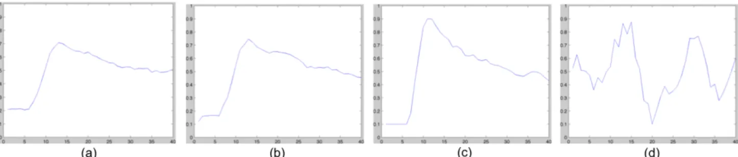
Fig. 1: Dynamic contrast enhanced time-series curves of (a) a liver tissue, (b)(c) non-liver tissues resembling curves of liver tissues (d) a region affected by motion, all normalized within an examination scanning series and after a low-pass filtering.
of the tissues being observed.
II. DCE-MRIANDTIME-SERIESANALYSIS
DCE-MRI has become an important tool for cancer diag-nosis and assessing therapeutic outcomes [6]. In acquiring DCE-MRI data, a contrast agent is injected into the patient during the MR image acquisition, so that the contrast of the successive images changes according to the observed tissue’s blood perfusion dynamics and vascular permeability. The change of image intensity over time is used to classify the type of the tissue of interest and to study its structure.
A. Time-Series Analysis
A time-series is often regarded as a point in multidimen-sional space. For a “similarity search” of time-series charac-teristics, the Euclidean distance is often employed, although the large dimensionality of typical time-series in the real-world makes such similarity analyses difficult. Thus there have been many approaches to reduce the dimensionality while preserv-ing the most important “features” in the reduced basis set. Use of the DWT (Discrete-Wavelet Transform) was suggested in [7] and a principal component analysis (PCA) based method was shown in [8]. Neural network methods for time-series analysis are summarised in [9] and clustering methods are summarised in [10]. Analysis is also often performed by fitting the time-series to a model.
B. Model-Based Approach
A widely used quantitative method for DCE-MRI analysis is a model-based approach. The change of contrast agent concentration appearing in an image over a time-course is modelled by for example
Ct(t) =Ktrans[Cp(t)⊗exp(−kept)], (1)
whereCt(t)is the observed contrast agent concentration in the
tissue at timet, Cp(t)is the tracer concentration in plasma,
Ktransrepresents the volume transfer constant between blood
plasma and extracellular extravascular space (EES) per minute,
kep is the rate constant between EES and blood plasma per
minute, and⊗represents a convolution over time [11]. Since the model itself is never a perfect description (due to the complexity of tissue structure and its inner behavior), once
the model is fit and parameters of the model are found, using this for classification can still be challenging.
C. Model-Free Approach
Model-free analyses such as the initial area under the curve (AUC) [12], are fairly simple to apply but cannot fully distinguish curves with different characteristics but having the same AUCs.
Neural-networks were used in [13]–[15] to obtain the ex-pected output classifying the types of tissues where the neural-networks are trained using a supervised dataset.
Chuang et al. [16] proposed the application of temporal clustering methods - Kohonen clustering network (KCN) and Fuzzy C-Means (FCM) - for the analysis of pulmonary per-fusion dynamics, which is also an unsupervised method used in DCE-MRI analysis similar to this study, but the clustering methods are computationally very expensive, making it inap-propriate for large-scale data analysis. Our method considers statistics over the entire large dataset rather than a single image or volume.
III. METHODS
A. Single-layer Sparse Autoencoder
Autoencoders have been applied to learning features for classification of more complex data such as visual [17]–[19] or audio recognition [4], where the parts of the entire system are given as the input to the autoencoder to build a convolution-net.
We use a single-layer sparse autoencoder to map our DCE-MRI time-series data in Ò40 to a compressed representation in 2Nh, where N
h is number of hidden nodes. We use the
binary representation of hidden units’ activation pattern for classification and visualization. The activation of each hidden unit is defined as
f(x) =g(W x+b), (2)
where g(z) = 1/(1 + exp(−z)) is the logistic sigmoid function, applied component-wise to the vector z, W is a weight vector between visible nodes and hidden nodes and
bis a bias.
The autoencoder with Nh hidden nodes is trained using
Fig. 2: The encoder-decoder setting as demonstrated for visual systems in [17] employed for time-series curves of liver tissues with 8 hidden units. The shape of typical liver time-series is reconstructed from the compressed representation.
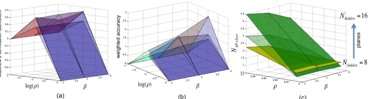
Fig. 3: Planes of Matthew’s correlation coefficient (a), weighted accuracy (b) and the number of activation patterns for detecting liver tissues (NAP=liver) (c), forNhidden={8,12,16}, which appear from the lowest to the highest.
with a term encouraging low average activation of the units [3], [5]. The overall cost function of the sparse autoencoder is
Jsparse(W, b) =J(W, b) +β
s2
X
j=1
KL(ρkρˆj), (3)
where J(W, b) is the likelihood cost function between the input and output of the autoencoder. The second term is the Kullback-Leibler (KL) divergence to encourage the average activation of each hidden unit ρˆj to be our desired level of
sparsity ρ with β being the sparsity penalty term and s2 number of hidden units. In minimizing the cost function over the entire dataset it learns sparse invariant features, the number of the features corresponding to the number of hidden units.
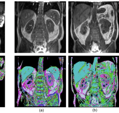
Fig. 4: Visualization of learned curve features with 16 hidden units and ρ = 0.01,β = 4on original training data (second row), and the acquired image before the contrast enhancement (first row). In the second row liver tumors are represented either black or as a complex pattern within the liver. The two columns are for the same patient from different visits.
Fig. 5: Visualization on a new dataset from a kidney study of a single patient with the 16 learned features. The different tissue types of kidney are well represented, and the main blood vessel within the healthy livers are shown as different colors from the livers. The false negative rate for this dataset in liver tissue detection was 0.07999 withfalse positiverate being 0.18905.
B. Training Data
For our training dataset, we used data from DCE-MRI study of tumors in different organs, where the majority are liver metastases. There were 46 scans (some were repeat scans of same patients) having 40 time-points in each DCE-MRI measurement, each time point producing an image vol-ume of 256×256×12 voxels, which corresponds to 22,080 (46×40×12) images.
For each image, background and regions affected by breath-ing motion are excluded and 1/16 of the remainbreath-ing curves were randomly sampled, resulting in about 1.6 million curves overall. No prior knowledge about the data was applied for training the dataset.
C. Pre-processing
The data was filtered with a low-pass filter to suppress noise, as is commonly performed in deep learning networks [3].
Some regions like the upper part of the liver are often affected by breathing motion. Their time-series curves appear like that in Fig.1 (d). They are excluded by applying logical operation to the pixels of the whole 40 time-scale images, where a pixel with less than 10% brightness of the whole brightness range of the image is regarded as the background and defined as false.
We have normalized our data by subtracting the mean of the entire curves and dividing by the standard deviation of its
elements over the entire curves collected. This normalization scheme was found to be much more effective than normalizing per volume or per patient etc.
D. Correlation within the Training Data
Although we sampled time-series curves randomly within an image slice, the slices were in a sequential order within the volume, and volumes were in the order of patients’ scans. It was therefore necessary to shuffle the order of the 1.6 million time-series curves to remove correlations within the training dataset, in order for the autoencoder to perform well for tissue type classification.
IV. RESULTS ANDANALYSIS
A. Visualization and Decoding
The binary digit activation pattern of the hidden layer is mapped into an RGB scale for visualization. The visualization result for our training dataset, and the corresponding original image before contrast enhancement are shown in Fig.4. Liver is always seen in the same color and liver tumors are rep-resented as highly variable patterns or black. Black color in the visualization means that there was no enhancement of the contrast agent for the tissue.
Fig. 6: (a) T1-map of an image from the training data showing with color scale0 <T1< 1200. (b) Fig.4 (a) after filtering with the T1 range of liver (500<T1<700).
Fig. 7: (a) T1-map of an image from the validation data showing in the range of 0< T1< 1200. (b) Fig.5 (b) after filtering with the T1 range of liver (550<T1<900).
liver in the color cyan. The kidneys are clearly differentiated as a combination of pink, blue and red colored regions, nicely representing the different tissue types within the kidney. The large blood vessel in the liver is also clearly differentiated from the liver as in Fig.5 (b).
The time-series curve of normal liver is reconstructed from the activation pattern of hidden units, called “shift-invariant representation” in [17], in Fig.2.
B. Validation and Performance Evaluation
To verify the reliability and repeatability of the method, as well as to measure the performance of the system, we drew regions-of-interest (ROIs) around the normal liver tissue of the new kidney dataset. We chose liver because liver is an organ with a wide homogeneous region of tissue characteristic making it easier to generate ROIs over large number of images “semi-automatically”, whereas other organs like kidney or heart are composed of a number of different tissue types making it harder to collect tissue sample points and verify. Curves of 7118 randomly sampled points in normal liver ROI were tested against 18519 randomly sampled non-liver curves. The performance was evaluated by measuring Matthew’s correlation coefficient (MCC) and weighted accuracy:
MCC=p T P×T N−F P×F N
(T P+F P)(T P+F N)(T N+F P)(T N+F N)
(4)
weighted accuracy=βAcc++ (1−β)Acc−
Acc+(True Positive Rate) = T P
T P +F N
Acc−(True Negative Rate) = T N
T N+F P,
(5)
where the T P, T N, F P and F N are True Positives, True Negatives, False Positives and False Negatives of detecting liver tissues respectively. The weightβwas set to 0.6, weight-ing more on predictweight-ing liver tissue correctly than pickweight-ing out non-liver tissues, as the classification result will possibly be integrated into a further processing or a more complex system for a more consistent detection of tissue types.
The performance measures of the whole parameter settings, with the measures of number of activation patterns for liver tissues(NAP=liver), are shown in Fig.3. The autoencoder clearly shows its peak performance withρ=0.01, whereas it generally performs well withβ=3 but theβ not as much affecting it as theρdoes. In Fig.3 (a), The peaks for the planes ofNhidden=
8 and 16 are found forβ=3. The reversed case for the plane of Nhidden=12 appears to arise either from the fact that the
training data was not enough or the samples didn’t represent the whole dataset very well. We think the same applies the same for the exceptional peak performance forlog(ρ)=-2 and
β=4 of the plane forNhidden=16 in Fig.3 (b).
It detects more activation patterns for liver tissue curves with lowerρ, higherβand more hidden units. HigherNAP=liver means clustering of the curves into more clusters, whereas lowerNAP=liver results in less clusters. The autoencoder shows generally better classification performance with higher number of hidden units.
The behaviour of the weight-decay parameter for the back-propagation of the autoencoder training to the performance was similar to that shown in [5], showing good performance for values smaller than 10−2 and less for larger values but not significantly affecting the performance, so it was not considered in the evaluation process. For all evaluations and visualizations, the value of10−3 was used.
It is interesting to notice the relation of the MCC and the NAP=liver. The MCC value +1 represents a perfect pre-diction, 0 an average random prediction and -1 an inverse prediction. Clustering the curves into too many clusters (too highNAP=liver) corresponds to a “random prediction”, whereas clustering into too few clusters (too low NAP=liver) results in an “inverse prediction”.
V. DISCUSSION
curves of liver and their similar non-liver tissues are clearly differentiated in their peak (about 20% higher for heart and aorta than liver) and the steepness of slope after the peak (heart and aorta have steeper slope after the peak than that of liver (Fig.1 (c)), while some are very similar to that of the liver (Fig.1 (b))).
This could be overcome with a careful selection of the parameters as was discussed in Sec.IV-B. Clustering of the curves into more clusters will result in a better discrimination of similar curve shapes, but at the same time in more activation patterns for a single tissue type, which will require a better classification strategy. Another option could be integrating the classification result into a more complex classification system, e.g. migrating these into a learning system of spatial features. Training with more data will improve performance as well, as the performance evaluation result varied with repeated training. As was discussed in Sec.IV-B, there were some unexceptional behaviours in the performance measure, which we think comes from the representational limitation of the sub-samples for the entire dataset. This issue could not be examined this time due to the limitation of time and our hardware, but could be investigated in a future work.
Inconsistency in medical data also contributes to the mis-classification. Unlike other visual systems, the properties of medical images differ significantly between cases even for a single patient study. For example, we have noticed that even for a single patient liver scan, liver tends to appear brighter for the images of slice locations where the liver is close to the centre of the image (Fig.4), whereas liver tends to appear darker for the slice locations where it is positioned towards the edge (Fig.5), known as the bias field effect resulting from the spatially varying sensitivity profile of the MRI receiver coils. The biological variability in the pre-contrast T1- maps is shown in Fig.6 (a) and Fig.7 (a). T1- value is more an abso-lute reflection of tissue characteristics than image brightness, although the absolute value varies by the scanned object or by the scanning environment. When we use the pre-contrast T1-value to filter the autoencoder classification, many of the false-positive voxels are eliminated as shown in Fig.6 (b) and Fig.7 (b), although at the cost of an increase in the false negative rate and the cost of selecting the right range of the T1- value for a particular volume.
Considering the variability in medical data and that the system worked well only with the normalization over the entire collected samples, pre-processing is a very important step for good classification performance of our system. Behaviour of parameter settings to performance was similar to other work with visual data.
VI. CONCLUSION
A single-layer sparse autoencoder was applied for time-series analysis in medical image analysis in an unsupervised manner, with analysis of its performance and behaviours with different settings of the model. The application of autoencoder to the time-series analysis of DCE-MRI allows complex char-acteristics of tissues to be represented and classified by a
com-pressed expression. Different tissue types can be classified and visualized without any supervision, from a large unlabelled medical image dataset.
ACKNOWLEDGMENT
We acknowledge the support received from the CRUK and EPSRC Cancer Imaging Centre in association with the MRC and Department of Health (England) grant C1060/A10334, also NHS funding to the NIHR Biomedical Research Centre.
REFERENCES
[1] I. Goodfellow, Q. Le, A. Saxe, H. Lee, and A. Ng, “Measuring invari-ances in deep networks,”Advances in neural information processing systems, vol. 22, pp. 646–654, 2009.
[2] C. MarcAurelio Ranzato, S. Chopra, and Y. LeCun, “Efficient learning of sparse representations with an energy-based model,”Advances in neural information processing systems, vol. 19, 2006.
[3] A. Coates, H. Lee, and A. Ng, “An analysis of single-layer networks in unsupervised feature learning,”Journal of Machine Learning Research, vol. 15, p. 48109.
[4] H. Lee, Y. Largman, P. Pham, and A. Ng, “Unsupervised feature learn-ing for audio classification uslearn-ing convolutional deep belief networks,”
Advances in neural information processing systems, vol. 22, pp. 1096– 1104, 2010.
[5] I. Goodfellow, Q. Le, A. Saxe, H. Lee, and A. Ng, “Measuring invari-ances in deep networks,”Advances in neural information processing systems, vol. 22, pp. 646–654, 2009.
[6] D. Collins and A. Padhani, “Dynamic magnetic resonance imaging of tumor perfusion,”Engineering in Medicine and Biology Magazine, IEEE, vol. 23, no. 5, pp. 65–83, 2004.
[7] K. Chan and A. Fu, “Efficient time series matching by wavelets,” in
Data Engineering, 1999. Proceedings., 15th International Conference on. IEEE, 1999, pp. 126–133.
[8] K. Yang and C. Shahabi, “A pca-based similarity measure for multivari-ate time series,” inProceedings of the 2nd ACM international workshop on Multimedia databases. ACM, 2004, pp. 65–74.
[9] G. Dorffner, “Neural networks for time series processing,” Neural Network World, vol. 6, no. 4, pp. 447–468, 1996.
[10] W. Liao et al., “Clustering of time series data–a survey,” Pattern Recognition, vol. 38, no. 11, pp. 1857–1874, 2005.
[11] S. Kety, “Theory of blood-tissue exchange and its application to mea-surement of blood flow,”Methods Med Res, vol. 8, pp. 223–227, 1960. [12] S. Walker-Samuel, M. Leach, and D. Collins, “Evaluation of response to treatment using dce-mri: the relationship between initial area under the gadolinium curve (iaugc) and quantitative pharmacokinetic analysis,”
Physics in Medicine and Biology, vol. 51, p. 3593, 2006.
[13] T. Twellmann, O. Lichte, and T. Nattkemper, “An adaptive tissue char-acterization network for model-free visualization of dynamic contrast-enhanced magnetic resonance image data,” Medical Imaging, IEEE Transactions on, vol. 24, no. 10, pp. 1256–1266, 2005.
[14] R. Lucht, M. Knopp, and G. Brix, “Classification of signal-time curves from dynamic mr mammography by neural networks* 1,”Magnetic Resonance Imaging, vol. 19, no. 1, pp. 51–57, 2001.
[15] R. Lucht, S. Delorme, and G. Brix, “Neural network-based segmenta-tion of dynamic mr mammographic images* 1,”Magnetic resonance imaging, vol. 20, no. 2, pp. 147–154, 2002.
[16] K. Chuang, M. Wu, Y. Lin, K. Hsieh, M. Wu, S. Tsai, C. Ko, and H. Chung, “Application of model-free analysis in the mr assessment of pulmonary perfusion dynamics,” Magnetic resonance in medicine, vol. 54, no. 2, pp. 299–308, 2005.
[17] M. Ranzato, F. Huang, Y. Boureau, and Y. Lecun, “Unsupervised learn-ing of invariant feature hierarchies with applications to object recog-nition,” inComputer Vision and Pattern Recognition, 2007. CVPR’07. IEEE Conference on. IEEE, 2007, pp. 1–8.
[18] H. Lee, C. Ekanadham, and A. Ng, “Sparse deep belief net model for visual area v2,” Advances in neural information processing systems, vol. 19, 2007.