Optimal Design and Control of Finite-Population
Queueing Systems
Chao Deng
A dissertation submitted to the faculty of the University of North Carolina at Chapel Hill in partial fulfillment of the requirements for the degree of Doctor of
Philosophy in the Department of Statistics and Operations Research.
Chapel Hill 2012
ABSTRACT
CHAO DENG: Optimal Design and Control of Finite-Population Queueing Systems (Under the direction of Professor Nilay Tanık Argon and Professor Vidyadhar G. Kulkarni)
We consider a service system with a finite population of customers (or jobs) and a service
resource with finite capacity. We model this finite-population queueing system by a closed
queueing network with two stages. The first stage, which represents the arrivals of customers
for service, consists of an automated station with ample capacity. The second stage, which
represents the service for customers, consists of multiple service stations which share the
finite service resource. We consider both discrete and continuous service resources. We are
interested in static or dynamic allocation of the service resource to the service stations in the
second stage in order to optimize a given system measure. Specifically, a static allocation
refers to a design problem, while a dynamic allocation refers to a control problem. In this
thesis, we study both.
For control problems, we specify a parallel-series structure for service stations. We first
consider dynamically allocating a single flexible server under both preemptive and
non-preemptive policies. We characterize the optimal policies of dynamically scheduling this
single server in order to maximize the long-run average throughput of the system. In the
special case of a series system, we show that the optimal policy is a sequential policy where
each customer is served by the single server sequentially from the first station until the
last one. For a parallel system, we show that there exists an optimal policy which gives
the highest priority to the station that has the largest service rate. We also propose an
index policy heuristic for the general parallel-series system and compare its performance
as opposed to the optimal policy by a numerical study. Finally, we study dynamically
allocating a finite amount of continuous service resource for the parallel system.
For design problems, we consider allocating a finite amount of service resource which
service times at a service station are exponentially distributed and their mean is a strictly
increasing and concave function of the allocated service resource. We characterize the
optimal allocation of the continuous resource in order to maximize the long-run average
throughput of the system. We first show that the system throughput is non-decreasing in
the number of customers. Then, we study the optimization problem in three cases depending
on the population size of customers in the system. First, when there is a single customer,
we show that the optimal allocation is given by a set of optimality equations. Secondly,
when the number of customers approaches infinity, we show that the optimal allocation
approaches to a limit. Finally, for any finite number of customers, we show that the system
throughput is bounded up by a limit. Moreover, under a certain condition, we show that
the system throughput function is Schur-concave.
ACKNOWLEDGEMENTS
I am sincerely grateful to my advisors, Professor Nilay Tanık Argon and Professor
Vidyadhar G. Kulkarni, for their direction and guidance over the past four years. They
taught me not only knowledge and methods, but more importantly, the attitudes toward
research. I would also like to thank my committee members, Professor Shankar Bhamidi,
Professor J. Scott Provan and Professor Serhan Ziya, for their inspiring suggestions on my
research.
Thanks to the faculty and staff of our lovely department, my sincere fellow graduate
students and those who have helped me throughout the years. They made my experience
in Chapel Hill a beautiful and unforgettable one.
Last, I would like to thank my wife, Yunhong Zhang, for her love and support over the
TABLE OF CONTENTS
Page
List of Figures . . . iii
Chapter 1: Introduction . . . 1
Chapter 2: Literature Review . . . 4
2.1 Dynamic Control . . . 4
2.1.1 Finite-Population and Closed Queueing Systems . . . 4
2.1.2 Open Queueing Systems . . . 6
2.2 Static Design . . . 8
Chapter 3: Optimal Dynamic Control of Finite-Population Queueing Systems: Reward Maximization . . . 10
3.1 Model Formulation . . . 10
3.2 Discrete Resource Constraint with a Single Server: Preemption . . . 13
3.2.1 Series System . . . 13
3.2.2 Parallel System . . . 21
3.3 Discrete Resource Constraint with a Single Server: Non-Preemption . . . 26
3.3.1 Series System . . . 26
3.3.2 Parallel System . . . 29
3.3.3 Two-Branch Three-Station System . . . 32
3.3.4 An Heuristic Policy and Numerical Results . . . 36
3.4 Continuous Resource . . . 38
3.5 Conclusion . . . 40
Chapter 4: Optimal Static Design of Finite-Population Queueing Systems: Through-put Maximization . . . 42
4.1 Model Formulation . . . 42
4.2 Characterization of Optimal Capacity Allocation . . . 46
4.2.1 A Single Job . . . 47
4.2.2 When Population Size Approaches Infinity . . . 49
4.2.3 Finite Population Size (1< B <∞) . . . 53
4.3 Conclusion . . . 56
Chapter 5: Optimal Dynamic Control of Finite-Population Queueing Systems: Waiting Cost Minimization . . . 57
5.1 A Parallel System with A Single Server . . . 57
5.2 A Parallel System with Continuous Resource . . . 63
Chapter 6: Future Research . . . 67
Bibliography . . . 69
LIST OF FIGURES
Figure Number Page
1.1 A closed queueing system with two stages of stations. . . 2
3.1 A closed queueing system with parallel-series service stations. . . 11 3.2 A closed queueing system with an automated station and K tandem service
stations. . . 14
3.3 A closed queueing system with an automated station and K parallel service stations. . . 21 3.4 Sample path couplings for the parallel system. . . 31
3.5 A closed queueing system with an automated station and three service stations. . 33
Chapter 1
INTRODUCTION
A finite-population queueing system, or sometimes called a finite-source queueing
sys-tem, is a queueing system in which requests for service are generated by a finite number
of customers (sources) and the requests are handled by a single or multiple server(s). The
service times of the requests generated by the customers are random variables. It is
as-sumed that the server can handle only one request at a time and uses a specified service
discipline. A customer can be idle, waiting for service, or in service. An idle customer
generates a request for service after a random amount of time independent of the states of
the other customers. Once the service is completed, the customer becomes idle again, and
the process repeats. In this thesis, we consider identical customers whose idle periods follow
an independent and identically distributed (i.i.d.) exponential distribution.
Two widely known applications of finite-population queueing systems are machine
inter-ference problems (or alternatively machine repairman problems) and computer-communication
systems. In the machine interference problems, the customers are machines. A machine
op-erates for a random period of time, then breaks down and requests service from workers.
While the worker resource is scarce, the service facility needs to make two decisions: which
worker will serve each machine and in what order the machines will be served. There is
a rich literature studying the machine interference problems. For a complete review of
research in this area, see the survey paper by Haque and Armstrong [7].
Many computer and communication systems can be modeled as finite-population
queue-ing systems. For example, in a computer-communication system, N terminals request to
use a computer (server) to process transactions. Each of the terminals takes a random time
to generate a request for the computer. The computer works on each of the transactions
and responds to the user at the terminal once the transaction is completed. The
through-put rate at which transactions are processed, or equivalently, generated in steady-state is
See Sztrik [30] for a complete review of finite-population queueing systems applications and
bibliography of related papers.
Finite-population queueing models can be also useful in developing effective policies in
healthcare. Green [5] provides an overview of using queueing analysis to improve service in
healthcare. For example, the finite-population queueing systems can be applied to the nurse
staffing problems in hospital wards. For the hospitals with high demands and constrained
resources, it is reasonable to assume that the number of patients staying is constant. Patients
stay in a bed for a random period of time, then request service from nurses. For a given
objective, for example, to maximize the steady-state processing rate of service requests, the
hospital managers need to determine service policies which optimally assign the nurses to
each of the requests.
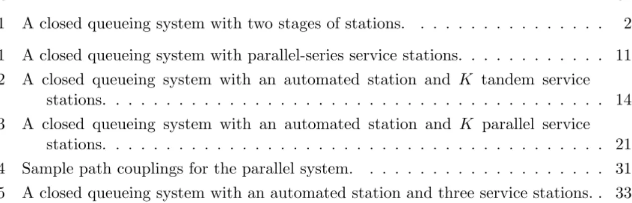
Figure 1.1: A closed queueing system with two stages of stations.
In this thesis, we are interested in optimal allocation of the resource capacity to stations
in a finite-population queueing system. We consider two management paradigms: dynamic
and static. Under the dynamic paradigm, we are allowed to change resource allocation
whenever the system changes its state. For the dynamic problems, we consider only
non-idling policies, i.e., a server cannot be idle if there is any service request waiting. Under the
static paradigm, allocation decisions are made before the system starts to operate. When
the system is under operation, we are not allowed to adjust resource allocation any more.
case, we assume that a finite amount of continuous service capacity can be used at any of
the service stations in the second stage. For the discrete case, we assume that there is a
single flexible server who is able to work at any of the service stations.
We model the finite-population service system by a closed queueing network withK+ 1
(2 ≤ K < ∞) stations (labeled as station 0,1,2, . . . , K) and a fixed population size of B
(1≤B <∞). These K+ 1 stations form the two stages of service, as shown in Figure 1.1,
where B jobs circulate between the two stages. The first stage consists of the automated
station, which is labeled as station 0, where B servers are dedicated to this station. A
customer receives service by one of the servers at station 0 immediately after she arrives
at this automated station. Assume that service times at station 0 are independent and
identically distributed with an exponential distribution and mean 1/µ0. The second stage
consists of the remaining K service stations, i.e., stations 1,2, . . . , K. We refer to theseK
stations in the second stage as service stations and to station 0 as an automated station.
Suppose that a fixed amount of resource is available to be used by service stations. The
decision is how to allocate the resource (statically or dynamically) to each of the service
stations in order to optimize a given system measure.
In this thesis, we mainly consider the objective of maximizing the long-run average
reward (throughput) of the system. We also conduct a brief study on dynamic control of
finite-population queueing systems under the objective of waiting cost minimization.
The organization of this thesis is given as follows. In Chapter 2, we provide a
litera-ture review on optimal control and design for finite-population queueing system and closed
queueing systems. In Chapter 3 and 4, we study the dynamic control problems and the
static design problems, respectively, under the reward (throughput) maximization
objec-tive. In Chapter 5, we present our work on dynamic control problems with the objective of
Chapter 2
LITERATURE REVIEW
Optimal design and control of queueing networks have been an important research
sub-ject of Operations Research for decades. In this chapter, we review the literature that is
most relevant to our work. We focus on the papers that study design and control problems
for closed queueing networks where finite-population service systems fit best. We also briefly
review the literature studying open queueing networks whose methodologies on design and
control problems are relevant to our work. In the review of each paper, we indicate the
following main features of the model considered by that paper:
1. Resource type (continuous, discrete single-server, or discrete multiple-server);
2. Objective function (e.g., throughput maximization or waiting cost minimization);
3. Policy constraints (e.g., preemption or non-preemption);
4. Structure of the queueing network (e.g., parallel or series);
5. The Results.
2.1 Dynamic Control
2.1.1 Finite-Population and Closed Queueing Systems
There is a rich literature that studies finite-population queueing systems and one of its
major applications, namely, the machine interference problem. A research survey on the
machine interference problem up to 1985 is provided by Stecke and Aronson [27]. Haque
and Armstrong [7] extensively extend this survey on this area until 2007. For a complete
literature review on finite-population queueing systems up to 2001, see Sztrik [30]. We here
Palesano and Chandra [21] study a machine interference problem with multiple types
of failures. A single server is available to work on all types of failures. A machine stays
functioning for a random time, then breaks down and requests service from the repairman.
The type of failures is random. This paper studies the system performance under different
service priorities by a numerical study and compares them. They do not prove any
optimal-ity results. They find that the mean number of machines waiting for repair increases when
the failure types with higher mean service times are given a high priority. This observation
is consistent with our work, in which we prove that the optimal policy that maximizes the
long-run system throughput rate gives priority to the stations with higher service rates.
Both Iravani and Kolfal [10] and Iravani, Krishnamurthy, and Chao [12] study a
single-server machine repairman problem with multiple classes of machines. The single single-server is
available to serve all machine classes. Iravani and Kolfal [10] consider preemptive policies.
Cost is incurred when a machine is waiting for service. The authors observe that in a
finite-population queueing system, ignoring customers’ arrival rate and applying thecµrule is not
always optimal to minimize the long-run average cost of the system. They find the conditions
under which static-priority rules, e.g. the cµ rule, are optimal independent of customer
arrival rate and customer population size. Iravani, Krishnamurthy, and Chao [12] consider
the non-preemptive case. Cost is incurred when a machine is down. The authors investigate
the dynamic assignment policies that minimize the total average customer waiting cost. The
authors show that the optimal service policy may never serve some classes of machines. For
those classes that are served, the paper shows that a static priority policy is optimal, and
derives sufficient conditions that determines the optimal priority sequence.
Iravani and Krishnamurthy [11] study a machine repairman problem with partially
cross-trained servers, i.e., each server is able to repair a set of machines. Cost is incurred when a
machine is down and waiting for repair. The objective is to obtain the optimal policy that
dynamically allocates servers to minimize the long-run average cost. The paper shows that
static machine priority rules are effective in minimizing the waiting cost rate.
Many papers study production systems by modeling them as closed serial queueing
networks. Koole and Righter [15] study a tandem manufacturing system with multiple
flexible servers. The tandem stations can be divided into several non-overlapping sets of
for optimal policies of dynamically assigning the server to work within his set of stations.
The objective is to maximize the departure process stochastically. They consider two cases
where either preemption and idling are permitted or preemption and idling are not allowed.
For both cases, they show that the optimal policy assigns each server to work at his last
nonempty station.
Hopp, Iravani, Shou and Lien [9] study a manufacturing system with a mix of manual and
automated equipment. The system operates under a constant work-in-process (CONWIP)
protocol, and is staffed by a single cross-trained worker. The system is modeled by a
tandem queueing network with three stations. The first station is an automated station
with automatic processing times but requiring a manual loading time. The other two
stations are manual stations requiring manual processing times. The single flexible server is
able to work at all stations. The paper investigates the optimal control policy to maximize
the average throughput rate. They show that the optimal control policy is a static priority
policy.
All papers reviewed in this section study dynamic control problems with a single server
or multiple servers. In other words, they consider discrete service resources in their models.
In this study, we consider both continuous and discrete service resources for our problems.
For the continuous resources, we assume that there is a fixed job processing capacity that
can be divided continuously among the K service stations in the second stage. For the
discrete resources, we assume that a single server or multiple servers are available to be
allocated among the K service stations.
2.1.2 Open Queueing Systems
There is a rich literature that studies design and control problems for open queueing
net-works. In this thesis, we only review those papers that are most relevant to our work. It is
important to point out that our focus is not open queueing networks but finite-population
and closed queueing networks.
Klimov [13] is a pioneering study on service priorities of open queueing networks. Klimov
[13] studies a dynamic control problem for an open queueing network with a finite number
of nodes and a single server. Jobs arrive according to a Poisson process at all nodes, and
in a queue. Interruption of service is not allowed. The paper proves that a priority index
policy is optimal in order to minimize the long-run average waiting cost. In a subsequent
paper, Klimov [14] provides a simple and efficient algorithm to compute such a priority
index for queueing networks with a forest structure.
Harrison [8] is another pioneering work on studying service priorities of open queueing
networks. Harrison [8] considers a single-server queue with multiple customer classes. He
assumes independent Poisson arrival processes. Service times have general distribution
which depend only on customer classes. Cost is incurred when a customer is waiting in
the system. A reward is gained when a customer is served. The objective is to maximize
the discounted total profit over an infinite planning horizon. A priority index policy called
modified static policy is shown to be optimal.
Van Oyen et al. [33] study a serial production system with flexible workers. Service
times are generally distributed and depend only on stations. The paper considers both
collaborative (servers are able to work together on one job) and non-collaborative (servers
are not allowed to work together on one job) cases. Under the collaborative case, they
show that the so-called expedite policy is optimal to minimize the cycle time for each
job. The expedite policy places all the servers successively on a given job. Under the
non-collaborative case, no optimal policy is found. However, they propose a so-called
pick-and-run policy and demonstrate that it is near-optimal. The paper also extends some their
insights to a capacity-constrained environment with a constant work-in-process protocol.
Andradottir et al. [2] consider dynamic control problems for multiple-server queueing
systems. Their objective is to find optimal dynamic allocation policies to maximize the
long-run average throughput. Travel times of servers between stations are negligible. They
show that all non-idling policies are optimal when service rates depend only on either servers
or stations. For a special two-station tandem queueing system with two flexible servers and
finite number of buffers between the two stations, the paper shows that the optimal policy
assigns one server to each station unless the first station is starved or the second station is
blocked. Andradottir and Ayhan [1] later extend this result to the case with three servers.
Yankovic and Green [35] explore the appropriate nurse-to-patient levels to minimize
the probability that a patient’s service request is delayed. They use a two-dimensional
system. However, this nurse staffing problem can also be another application for
finite-population queueing systems. We consider a finite-finite-population queueing system with four
service stations representing patients’ admission, patients’ stay in beds, patients’ caring
requests and patients’ discharge. While this paper seeks an appropriate nurse-to-patient
level for hospitals, we are interested in obtaining priority policies that optimally assign the
nurses to each of the patient requests in order to achieve a given objective. Finite-population
queueing systems can be used to model the hospital systems if we assume that the number
of patients staying in the hospitals is constant.
2.2 Static Design
In this section, we review articles that study static workload or server allocation problems
of closed queueing systems. Stecke and Morin [28] investigate optimality of balancing
work-loads in closed queueing systems. They consider a central server closed queueing network
where stations are parallel to each other. They are interested in obtaining optimal policies
for allocating workload in order to maximize the system throughput. The paper proves that
the throughput of this system is a quasi-concave function of workloads, and shows that a
balanced allocation of workloads maximizes the expected throughput of the system.
Stecke [26] studies the non-concavity property of throughput function in closed queueing
networks. For a general-structured closed queueing network with multiple customers, she
shows that the throughput function is not concave in workload. When the closed queueing
network includes two single server stations, the paper proves that the throughput function is
concave when there are two customers, and the throughput function is quasi-concave when
there are more than two customers.
Yao [36] considers a closed queueing network with single-server stations and exponential
service times. He investigates the concavity property of the long-run average throughput
of the system. He proves that the system throughput as a function of loading is
Schur-concave. As a consequence, the paper shows that, when the total loading of the system is
a constant, the balanced (or equal) loading maximizes the system throughput based on the
majorization property.
Shanthikumar and Yao [25] study the static allocation problem of a multiple-server
to maximize throughput. The paper shows that the throughput of the system has a
mono-tonicity property, which means that an optimal policy allocates more servers to a station
with a higher workload. They provide a search algorithm to obtain an optimal policy within
a small number of allocations satisfying the monotonicity property.
Lee, Srinivasan, and Yano [17] consider the problem of allocating workload in a closed
queueing network with multi-server stations. Their objective is to maximize the
long-run average throughput of the system. The paper assumes that the system throughput is
product-form and there is a single class of customers. The paper proves that the throughput
function is quasi-concave in workload for a single-server closed queueing network and a
multi-server closed queueing network with two customers. For the general model, the authors
develop two heuristic algorithms to search the optimal workload allocation.
These papers study static allocation problems of closed queueing networks where all
stations are included for allocation decisions. In this study, we consider a two-stage queueing
system where the first stage is a special automated station. Allocation decisions are made
only for the service stations in the second stage. Furthermore, except for Shanthikumar
and Yao’s paper [25], the other papers consider allocating the workload in the system. In
this thesis, we consider allocating a fixed amount of service resource, and we study both
Chapter 3
OPTIMAL DYNAMIC CONTROL OF
FINITE-POPULATION QUEUEING SYSTEMS: REWARD
MAXIMIZATION
In this chapter, we study dynamic control problems, i.e., we are allowed to change
resource allocation when the system changes its state. We consider both preemptive and
non-preemptive policies. Let ΠP and ΠN P denote the set of preemptive policies and
non-preemptive policies, respectively. For non-preemptive policies, the server is allowed to make
service decisions whenever a service at the automated station or the service stations is
completed. Under non-preemptive policies, the server is allowed to switch to work at other
stations only when it completes service. In this chapter, we only consider non-idling policies,
i.e., the server (or service capacity) is not allowed to be idle whenever job(s) are available
at the service stations.
We formulate the dynamic control problem in Section 3.1. In Sections 3.2 and 3.3, we
consider the case where the service resource is discrete and a single server is available to
work at K service stations. We study preemptive and non-preemptive policies in Section
3.2 and 3.3, respectively. In Section 3.4, we consider the problem with continuous resource
constraint.
3.1 Model Formulation
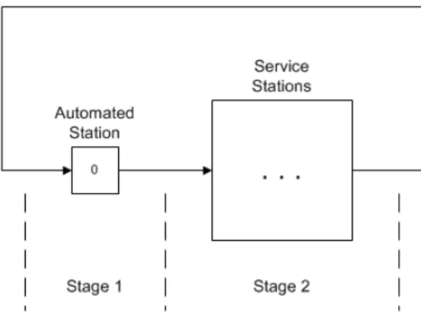
We consider a special case of the general finite-population queueing system, called a parallel-series system, as shown in Figure 3.1. The second stage in this system consists of M
parallel branches, where the m-th branch consists of im service stations in series. We use
an M-dimensional vector (i1, i2, . . . , iM) to denote the parallel-series system which has M
service types (branches) and im tasks on its m-th branch (m = 1,2, . . . , M), satisfying
PM
m=1im = K. For example, a system with M = 1 and i1 = K represents a tandem
represents a parallel queueing network withM service stations. Such a parallel-series system
arises where the service needs can be classified intoM types. Them-th service type consists
of a series of im tasks, each taking a random amount of time.
Figure 3.1: A closed queueing system with parallel-series service stations.
We denote the ith node in the m-th branch as node (i, m). A customer stays in node
0 for a random amount of time and then moves to node (1, m) with probability pm > 0
(1 ≤ m ≤ M), where PM
m=1pm = 1. A customer stays in node (i, m) until she receives
service from the server, then moves to node (i+ 1, m) if i < im, and to node 0 if i =im.
This process repeats forever. Let Sj,m represent the random service time performed by the
server in node (j, m) (1 ≤ j ≤ im, 1 ≤ m ≤ M). We assume that all service times are
independent of each other.
LetD0π(t) and D(πi,m)(t) denote the number of service completions in node 0 and in node
(i, m) (1≤i≤im, 1≤m≤M), respectively during [0, t] under policyπ, where π is either
in ΠP or ΠN P. Suppose that a finite reward R(i,m) is gained when service is completed in
node (i, m) (1≤i≤im, 1≤m≤M). We define
Rπ ≡lim inf
t→∞
M
X
m=1
im
X
i=1
R(i,m)Dπ(i,m)(t)
t , (3.1.1)
LetT H0π denote the long-run average throughput of station 0 under policyπ, i.e.,
T H0π ≡lim inf
t→∞
D0π(t)
t . (3.1.2)
Throughout the paper, we will refer to T H0π as the system throughput. We first show
that maximizing the long-run average reward of the system is equivalent to maximizing the
long-run average throughput of the system.
Theorem 3.1.1. For the parallel-series system, maximizing the long-run average reward of the system is equivalent to maximizing the long-run average throughput of the system.
Proof of Theorem 3.1.1. We define T H(πi,m) as the long-run average throughput from
node (i, m), i.e.,
T H(πi,m)≡lim inf
t→∞
Dπ(i,m)(t)
t .
We first show that the long-run average throughput at any two consecutive nodes are equal,
i.e., T H(πi,m) =T H(πi+1,m) (1≤i≤im−1, 1≤m ≤M). Let C(πi,m)(t) denote the number
of customers in node (i, m) at timet(1≤i≤im and 1≤m≤M). Then, we have
C(πi+1,m)(t) =C(πi+1,m)(0) +Dπ(i,m)(t)−Dπ(i+1,m)(t), for 1≤i≤im−1 and 1≤m≤M,
which implies
lim inf
t→∞
Dπ
(i,m)(t)
t = lim inft→∞
Dπ
(i+1,m)(t)
t + lim inft→∞
Cπ
(i+1,m)(t)
t −lim inft→∞
Cπ
(i+1,m)(0)
t . (3.1.3)
Since C(πi+1,m)(t) ≤ B < ∞ for all t ≥ 0, the last two terms in (3.1.3) are equal to 0.
Hence,
T H(πi,m)=T H(πi+1,m), for 1≤i≤im−1 and 1≤m≤M. (3.1.4)
Now, let Dπ0,m(t) be the number of customers who request an m-th type of service after
leaving node 0 during [0, t] under policy π, and hence PM
m=1Dπ0,m(t) = Dπ0(t). A similar
argument as above leads to
lim inf
t→∞
D0π,m(t)
t = lim inft→∞
Dπ(1,m)(t)
t .
By the law of large numbers, we know that
lim inf
t→∞
D0π,m(t)
and hence using (3.1) we have
T H(1π,m)=pmT H0π. (3.1.5)
By (3.1.4) and (3.1.5), we can show that
Rπ = lim inf
t→∞ M X m=1 im X i=1
R(i,m)D(πi,m)(t)
t = M X m=1 im X i=1
R(i,m)T H(πi,m)
=
M
X
m=1
T H(1π,m)
im
X
i=1 R(i,m)
=T H0π
M X m=1 pm im X i=1
R(i,m).
SincePM
m=1pmPimi=1R(i,m) is a constant for givenR(i,m)andpm (1≤i≤im, 1≤m≤M),
maximizing Rπ is equivalent to maximizing T H0π.
In the following discussions, our objective is to solve the following two optimization
problems in order to maximize the long-run average throughput of the system:
max
π∈ΠP
T H0π
and
max
π∈ΠN P
T H0π.
3.2 Discrete Resource Constraint with a Single Server: Preemption
In this section, we consider allocating a single flexible server under preemptive policies.
Assume that service times at station k are exponentially distributed with rate µk where
0< µk<∞.
3.2.1 Series System
We first study a series system as shown in Figure 3.2. We formulate the optimization
problem as a Markov decision process. Let n = (n1, n2, . . . , nK) denote the state of the
system, wherenk≥0 represents the number of jobs at stationk(1≤k≤K, 0≤PKj=1nj ≤
B). Letn=PK
In ⊆ {1,2, . . . , K} denote the set of service stations that are non-empty in state n. Also,
let ei denote aK-dimensional row vector with all elements 0 except where theith element
is equal to 1, and denote by 0 a K-dimensional row vector with all elements equal to 0.
DefineV(n) as the bias of staten, andgas the long-run average throughput of the system.
Figure 3.2: A closed queueing system with an automated station and K tandem service stations.
Because both the state space and the action space are finite and the transition matrix
consists of a single recurrent class for every deterministic stationary policy, the MDP under
study is unichain. Hence, we know that there exists a stationary average optimal policy
and henceg exists (see, e.g., Theorem 8.4.5 in Puterman [22]). Define Λ =Bµ0+PKk=1µk
as the uniformization constant. Without loss of generality, we assume that Λ = 1. Then,
the optimality equation can be expressed as follows:
g+V(n) = (B−n)µ0V(n+e1) +nµ0V(n) +f(n), for 0≤n≤B, (3.2.1)
where
f(n) =
K
X
k=1
µkV(n) +
0, ifn=0
maxi∈In
n
µi[V(n−ei+ei+1)−V(n)]1{i6=K},
µK[V(n−eK) + 1−V(n)]1{i=K}
o
, otherwise,
where1{A} is an indicator function with value of 1 ifAholds or value of 0 otherwise. Here,
we use the fact that the throughput from each station in a tandem line is the same (see the
proof of Theorem 3.1.1). We provide a complete characterization of the optimal policy in
Theorem 3.2.1.
Proof of Theorem 3.2.1. In order to prove Theorem 3.2.1, we first show that the result holds for a similar finite horizon problem given by (3.2.2) withmperiods for all m≥0. Let
Nk denote the state of the system at period k anddk(Nk) the decision rule at periodk in
state Nk under policy π. Let r(N, d) denote the gained throughput when the system is in
stateN and the actiondis taken. We defineVm(π,n) as them-period expected throughput
under policy π when the initial state is n, i.e.,
Vm(π,n)≡E
"m−1 X
k=0
r(Nk, dk(Nk))
# .
Then, the optimal m-period expected total throughput is
Vm∗(n)≡ sup
π∈ΠP
Vm(π,n). (3.2.2)
We let g(π,n) be the long-run average throughput under policy π, given that the initial
state of the system is n, i.e.,
g(π,n)≡lim inf
m→∞
1
mVm(π,n).
Let µ ≡PK
k=1µk. Then, the optimality equation for the finite-period problem can be
expressed as follows. For all m≥0,
Vm+1(n) = (B−n)µ0Vm(n+e1) +nµ0Vm(n) +fm(n), for 0≤n≤B, (3.2.3)
where
fm(n) =µVm(n) +
0, ifn=0
maxi∈In
n
[µiVm(n−ei+ei+1)−µiVm(n)]1{i6=K},
[µK(Vm(n−eK) + 1)−µKVm(n)]1{i=K}
o
, otherwise.
We assume that V0(n) = 0 for all n. For system state n, where 2 ≤ n≤ B, let l1(n) ≡
max{k :k ∈In} and l2(n) ≡max{k: k∈ In−el1(n)}. We will show that, for all m ≥ 0,
2≤n≤B, and j∈In−el1(n),
i. ifl1(n)< K,
µl1(n)Vm(n−el1(n)+el1(n)+1)−µjVm(n−ej+ej+1) + (µj−µl1(n))Vm(n)≥0;
ii. if l1(n) =K,
µKVm(n−eK)−µjVm(n−ej+ej+1) + (µj−µK)Vm(n)≥ −µK; (3.2.5)
iii.
Vm(n+e1)−Vm(n)≥0. (3.2.6)
We will use induction onm. BecauseV0(n) = 0 for alln, the inequalities automatically
hold at period 0. Assume that the inequalities hold at period m. We will show that they
also hold at period m+ 1. In the remainder of this proof, we will let i=l1(n) for ease of
notation whenever it does not cause any ambiguity.
Proof of (3.2.4): We will consider two cases.
(a) Suppose that l1(n)< K−1. Using equation (3.2.3), we have
µiVm+1(n−ei+ei+1)−µjVm+1(n−ej+ej+1) + (µj−µi)Vm+1(n)
=(B−n)µ0[µiVm(n−ei+ei+1+e1)−µjVm(n−ej+ej+1+e1) + (µj−µi)Vm(n+e1)]
+nµ0[µiVm(n−ei+ei+1)−µjVm(n−ej+ej+1) + (µj−µi)Vm(n)]
+µi+1µiVm(n−ei+ei+2)−µiµjVm(n−ej+ej+1−ei+ei+1)
+µi(µj−µi)Vm(n−ei+ei+1)
+ (µ−µi+1)µiVm(n−ei+ei+1)−(µ−µi)µjVm(n−ej+ej+1)
+ (µ−µi)(µj−µi)Vm(n)
=(B−n)µ0[µiVm(n−ei+ei+1+e1)−µjVm(n−ej+ej+1+e1) + (µj−µi)Vm(n+e1)]
+µi[µi+1Vm(n−ei+ei+2)−µjVm(n−ej+ej+1−ei+ei+1)
+ (µj−µi+1)Vm(n−ei+ei+1)]
+ (nµ0+µ−µi)[µiVm(n−ei+ei+1)−µjVm(n−ej+ej+1) + (µj −µi)Vm(n)],
which is non-negative by the inductive hypothesis for (3.2.4) at period m, the facts
that l1(n+e1) = l1(n) and l1(n−ei +ei+1) = i+ 1, and the assumption that
(b) Suppose that l1(n) =K−1. Using equation (3.2.3), we have
µK−1Vm+1(n−eK−1+eK)−µjVm+1(n−ej+ej+1) + (µj −µK−1)Vm+1(n)
=(B−n)µ0[µK−1Vm(n−eK−1+eK+e1)−µjVm(n−ej+ej+1+e1)
+ (µj −µK−1)Vm(n+e1)]
+nµ0[µK−1Vm(n−eK−1+eK)−µjVm(n−ej+ej+1) + (µj−µK−1)Vm(n)]
+µKµK−1[Vm(n−eK−1) + 1]−µK−1µjVm(n−ej+ej+1−eK−1+eK)
+µK−1(µj−µK−1)Vm(n−eK−1+eK)
+ (µ−µK)µK−1Vm(n−eK−1+eK)−(µ−µK−1)µjVm(n−ej+ej+1)
+ (µ−µK−1)(µj −µK−1)Vm(n)
=(B−n)µ0[µK−1Vm(n−eK−1+eK+e1)−µjVm(n−ej+ej+1+e1)
+ (µj −µK−1)Vm(n+e1)]
+µK−1[µKVm(n−eK−1)−µjVm(n−ej+ej+1−eK−1+eK)
+ (µj −µK)Vm(n−eK−1+eK) +µK]
+ (nµ0+µ−µK−1)[µK−1Vm(n−eK−1+eK)−µjVm(n−ej+ej+1)
+ (µj −µK−1)Vm(n)],
which is non-negative by the inductive hypothesis for (3.2.4) and (3.2.5) at periodm,
the facts that l1(n+e1) = K−1 and l1(n−eK−1+eK) =K, and the assumption
that Bµ0+µ=1.
(a) Suppose that l2(n) =K. Using equation (3.2.3), we have
µKVm+1(n−eK)−µjVm+1(n−ej+ej+1) + (µj−µK)Vm+1(n)
=(B−n+ 1)µ0µKVm(n−eK+e1)
+ (B−n)µ0[−µjVm(n−ej+ej+1+e1)) + (µj−µK)Vm(n+e1)]
+ (n−1)µ0µKVm(n−eK) +nµ0[−µjVm(n−ej+ej+1) + (µj −µK)Vm(n)]
+µKµK−µjµK+ (µj−µK)µK
+µK[µKVm(n−2eK)−µjVm(n−ej +ej+1−eK) + (µj−µK)Vm(n−eK)]
+ (µ−µK)[µKVm(n−eK)−µjVm(n−ej+ej+1) + (µj−µK)Vm(n)]
=(B−n)µ0[µKVm(n−eK+e1)−µjVm(n−ej+ej+1+e1) + (µj−µK)Vm(n+e1)]
+µ0[µKVm(n−eK+e1)−µjVm(n−ej+ej+1) + (µj−µK)Vm(n)]
+µK[µKVm(n−2eK)−µjVm(n−ej +ej+1−eK) + (µj−µK)Vm(n−eK)]
+ ((n−1)µ0+µ−µK)[µKVm(n−eK)−µjVm(n−ej+ej+1) + (µj−µK)Vm(n)],
which is greater than or equal to −µK by the inductive hypothesis for (3.2.5) and
(3.2.6) at period m, the facts that l1(n+e1) = K and l1(n−eK) = K, and the
assumption thatBµ0+µ=1.
(b) Suppose that l2(n)< K. Using equation (3.2.3), we have
µKVm+1(n−eK)−µjVm+1(n−ej+ej+1) + (µj−µK)Vm+1(n)
=(B−n+ 1)µ0µKVm(n−eK+e1)
+ (B−n)µ0[−µjVm(n−ej +ej+1+e1)) + (µj−µK)Vm(n+e1)]
+ (n−1)µ0µKVm(n−eK) +nµ0[−µjVm(n−ej+ej+1) + (µj−µK)Vm(n)]
−µjµK+ (µj−µK)µK
+µKµl2(n)Vm(n−eK−el2(n)+el2(n)+1)−µjµKVm(n−ej+ej+1−eK)
+ (µj−µK)µKVm(n−eK)
+µK(µ−µl2(n))Vm(n−eK)−µj(µ−µK)Vm(n−ej+ej+1)
=(B−n)µ0[µKVm(n−eK+e1)−µjVm(n−ej+ej+1+e1) + (µj−µK)Vm(n+e1)]
+µ0[µKVm(n−eK+e1)−µjVm(n−ej+ej+1) + (µj−µK)Vm(n)]
+ (n−1)µ0[µKVm(n−eK)−µjVm(n−ej+ej+1) + (µj−µK)Vm(n)]
+µK[µl2(n)Vm(n−eK−el2(n)+el2(n)+1)−µjVm(n−ej+ej+1−eK)
+ (µj−µl2(n))Vm(n−eK)−µK]
+ (µ−µK)[µKVm(n−eK)−µjVm(n−ej+ej+1) + (µj−µK)Vm(n)],
which is greater than or equal to−µK by the inductive hypothesis for (3.2.4), (3.2.5)
and (3.2.6) at period m, the facts that l1(n+e1) =K and l1(n−eK) =l2(n)< K,
and the assumption thatBµ0+µ=1.
Proof of (3.2.6). We will consider two cases:
(a) Suppose that l1(n)< K. Using equation (3.2.3), we have
Vm+1(n+e1)−Vm+1(n)
=(B−n−1)µ0Vm(n+ 2e1)−(B−n)µ0Vm(n+e1)
+ (n+ 1)µ0Vm(n+e1)−nµ0Vm(n)
+µl1(n)[Vm(n+e1−el1(n)+el1(n)+1)−Vm(n−el1(n)+el1(n)+1)]
+ (µ−µl1(n))[Vm(n+e1)−Vm(n)]
=(B−n−1)µ0[Vm(n+ 2e1)−Vm(n+e1)]
+µl1(n)[Vm(n+e1−el1(n)+el1(n)+1)−Vm(n−el1(n)+el1(n)+1)]
+ (nµ0+µ−µl1(n))[Vm(n+e1)−Vm(n)],
which is non-negative by the inductive hypothesis for (3.2.6) at period m and the
(b) Suppose that l1(n) =K. Using equation (3.2.3), we have
Vm+1(n+e1)−Vm+1(n)
=(B−n−1)µ0Vm(n+ 2e1)−(B−n)µ0Vm(n+e1)
+ (n+ 1)µ0Vm(n+e1)−nµ0Vm(n)
+µK[Vm(n+e1−eK)−Vm(n−eK)]
+ (µ−µK)[Vm(n+e1)−Vm(n)]
=(B−n−1)µ0[Vm(n+ 2e1)−Vm(n+e1)]
+µK[Vm(n+e1−eK)−Vm(n−eK)]
+ (nµ0+µ−µK)[Vm(n+e1)−Vm(n)],
which is non-negative by the inductive hypothesis for (3.2.6) at period m and the
assumption thatBµ0+µ=1.
Letπ∗ be the policy that gives priority to the non-empty station with the largest index
in the series system. By (3.2.4) and (3.2.5), we have
Vm(π∗,n)≥Vm(π,n) (3.2.7)
for all π∈ΠP and for allm≥0. Dividing both sides of (3.2.7) by m and taking limits as
m approaches infinity the long-run average throughput result follows, i.e.,
g(π∗,n)≥g(π,n)
for allπ ∈ΠP. Hence, policyπ∗ maximizes the long-run average throughput of the system.
Remarks. Theorem 3.2.1 shows that we should put the server to work at the station
which is as close to the entry into station 0 as possible when a job is available. The intuition
is that the earlier a job goes back to the automated station, the earlier this job leaves station
0 to request for service, which increases the utilization of the server and the throughput of
the system as well. Note that the optimal policy eventually becomes a policy under which
the server picks a job from the queue in front of station 1 and completes the service of this
job at all service stations 1,2, . . . , K before it starts working on another job waiting in front
In the set of preemptive policies, the optimal policy for the series system shown in
Theorem 3.2.1 is actually non-preemptive. The server works on a job from the first station
to last station sequentially without being interrupted by new arrivals from station 0. Hence,
the sequential policy is also optimal within ΠN P under the Markovian case.
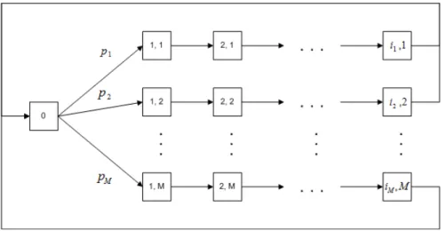
3.2.2 Parallel System
Next, we study a parallel system as shown in Figure 3.3. We formulate the optimization
problem as a Markov decision process (MDP). We use the same notation defined in Section
Figure 3.3: A closed queueing system with an automated station and K parallel service stations.
3.2.1 unless otherwise stated. Following the same argument, we know that there exists a
stationary average optimal policy and henceg exists. Without loss of generality, we assume
that Λ = 1. Then, the optimality equation can be expressed as follows:
g+V(n) = (B−n)µ0
K
X
k=1
pkV(n+ek) +nµ0V(n) +f(n), for 0≤n≤B, (3.2.8)
where
f(n) =
K
X
k=1
µkV(n) +
0 ifn=0,
maxi∈In{µi(V(n−e
i) + 1)−µ
iV(n)} otherwise.
Theorem 3.2.2. Suppose that there exists a station i for which µi ≥ µj, for all j =
1,2, . . . , K and j6=i. Then, there exists an optimal policy which gives the highest priority to station i within the set of all preemptive policiesΠP.
Proof of Theorem 3.2.2. In order to prove Theorem 3.2.2 we show that the result holds
for them-period expected total throughput problem defined by (3.2.2) for all m≥0. Then,
the optimality equation for the finite-period problem can be expressed as follows. For all
m≥0,
Vm+1(n) = (B−n)µ0
K
X
k=1
pkVm(n+ek) +nµ0Vm(n) +fm(n), for 0≤n≤B, (3.2.9)
where
fm(n) = K
X
k=1
µkVm(n) +
0 ifn=0,
maxi∈In{µi(Vm(n−e
i) + 1)−µ
iVm(n)} otherwise.
We assume that V0(n) = 0 for all n.
Without loss of generality, we assume that µ1 ≥µj, for all j= 2,3, . . . , K. For system
staten, where 2≤n≤B, letl1(n)≡min{k:k∈In} and l2(n)≡min{k:k∈In−el1(n)}.
Let na=n+ea (1≤a≤K). We will show that, for all m ≥0, 2≤n≤B,n1 ≥1, and
1≤a≤K,
µ1Vm(n−e1)−µjVm(n−ej) + (µj−µ1)Vm(n)≥µj −µ1, (3.2.10)
µ1Vm(na−e1)−µjVm(na−ej) + (µj−µ1)Vm(n)≥µj −µ1, (3.2.11)
where j 6= 1 and j ∈In. We will use induction on m. Since V0(n) = 0 for all n, (3.2.10)
and (3.2.11) automatically hold at period 0. Assume that inequalities (3.2.10) and (3.2.11)
hold at period m. We will show that they also hold at period m+ 1.
(a) Suppose that l2(n) = 1. Using equation (3.2.9), we have
µ1Vm+1(n−e1)−µjVm+1(n−ej) + (µj −µ1)Vm+1(n)
=(B−n+ 1)µ0 X
k
pk[µ1Vm(n−e1+ek)−µjVm(n−ej+ek))]
+ (B−n)µ0 X
k
pk(µj−µ1)Vm(n+ek)
+ (n−1)µ0[µ1Vm(n−e1)−µjVm(n−ej)] +nµ0[(µj−µ1)Vm(n)]
+µ1µ1−µjµ1+ (µj−µ1)µ1+µ1[µ1Vm(n−2e1)−µjVm(n−ej−e1)
+ (µj−µ1)Vm(n−e1)]
+ (µ−µ1)[µ1Vm(n−e1)−µjVm(n−ej) + (µj−µ1)Vm(n)]
=(B−n)µ0 X
k
pk[µ1Vm(n−e1+ek)−µjVm(n−ej+ek) + (µj−µ1)Vm(n+ek)]
+µ0 X
k
pk[µ1Vm(n−e1+ek)−µjVm(n−ej+ek)) + (µj−µ1)Vm(n)]
+µ1[µ1Vm(n−2e1)−µjVm(n−ej −e1) + (µj−µ1)Vm(n−e1)]
+ ((n−1)µ0+µ−µ1)[µ1Vm(n−e1)−µjVm(n−ej) + (µj−µ1)Vm(n)],
which is greater than or equal to µj−µ1 by the inductive hypothesis for (3.2.10) and
(3.2.11) at period m, the fact that µ1 ≥µj for all j ∈In, and the assumption that
Bµ0+µ= 1.
(b) Suppose that l2(n)>1. Using equation (3.2.9), we have
µ1Vm+1(n−e1)−µjVm+1(n−ej) + (µj −µ1)Vm+1(n)
=(B−n+ 1)µ0 X
k
pk[µ1Vm(n−e1+ek)−µjVm(n−ej+ek))]
+ (B−n)µ0 X
k
pk(µj−µ1)Vm(n+ek)
+ (n−1)µ0[µ1Vm(n−e1)−µjVm(n−ej)] +nµ0(µj−µ1)Vm(n)
+µ1µl2(n)−µjµ1+ (µj−µ1)µ1
+µ1µl2(n)Vm(n−e1−el2(n))−µjµ1Vm(n−ej −e1) + (µj−µ1)µ1Vm(n−e1)
=(B−n)µ0 X
k
pk[µ1Vm(n−e1+ek)−µjVm(n−ej+ek) + (µj−µ1)Vm(n+ek)]
+µ0 X
k
pk[µ1Vm(n−e1+ek)−µjVm(n−ej+ek)) + (µj−µ1)Vm(n)]
+µ1[µl2(n)Vm(n−e1−el2(n))−µjVm(n−ej−e1) + (µj−µl2(n))Vm(n−e1)
+µl2(n)−µ1]
+ ((n−1)µ0+µ−µ1)[µ1Vm(n−e1)−µjVm(n−ej) + (µj−µ1)Vm(n)],
which is greater than or equal to µj−µ1 by the inductive hypothesis for (3.2.10) and
(3.2.11) at period m andl2(n) =l1(n−e1), the fact that µ1 ≥µj for allj∈In, and
the assumption thatBµ0+µ= 1.
Proof of (3.2.11). We will consider two cases:
(a) Suppose that l2(na) = 1. Using equation (3.2.9), we have
µ1Vm+1(na−e1)−µjVm+1(na−ej) + (µj−µ1)Vm+1(n)
=(B−n)µ0X
k
pk[µ1Vm(na−e1+ek)−µjVm(na−ej+ek))]
+ (B−n)µ0X
k
pk[(µj−µ1)Vm(n+ek)]
+nµ0[µ1Vm(na−e1)−µjVm(na−ej)]
+nµ0[(µj−µ1)Vm(n)]
+µ1µ1−µjµ1+ (µj−µ1)µ1
+µ1µ1Vm(na−2e1)−µjµiVm(na−ej−e1) + (µj −µ1)µ1Vm(n−e1)
+µ1(µ−µ1)Vm(na−e1)−µj(µ−µi)Vm(na−ej) + (µj −µ1)(µ−µ1)Vm(n)
=(B−n)µ0 X
k
pk[µ1Vm(na−e1+ek)−µjVm(na−ej+ek) + (µj−µ1)Vm(n+ek)]
+nµ0[µ1Vm(na−e1)−µjVm(na−ej) + (µj−µ1)Vm(n)]
+µ1[µ1Vm(na−2e1)−µjVm(na−ej−e1) + (µj−µ1)Vm(n−e1)]
+ (µ−µ1)[µ1Vm(na−e1)−µjVm(na−ej) + (µj −µ1)Vm(n)],
which is greater than or equal to µj−µ1 by the inductive hypothesis for (3.2.11) at
(b) Suppose that l2(na)>1. Using equation (3.2.9), we have
µ1Vm+1(na−e1)−µjVm+1(na−ej) + (µj−µ1)Vm+1(n)
=(B−n)µ0 X
k
pk[µ1Vm(na−e1+ek)−µjVm(na−ej+ek))]
+ (B−n)µ0 X
k
pk[(µj−µ1)Vm(n+ek)]
+nµ0[µ1Vm(na−e1)−µjVm(na−ej)] +nµ0[(µj −µ1)Vm(n)]
+µ1µl2(na)−µjµ1+ (µj−µ1)µ1
+µ1µl2(na)Vm(na−e1−el2(n a)
)−µjµ1Vm(na−ej−e1) + (µj−µ1)µ1Vm(n−e1)
+µ1(µ−µl2(na))Vm(na−e1)−µj(µ−µ1)Vm(na−ej) + (µj−µ1)(µ−µ1)Vm(n)
=(B−n)µ0 X
k
pk[µ1Vm(na−e1+ek)−µjVm(na−ej+ek) + (µj−µ1)Vm(n+ek)]
+nµ0[µ1Vm(na−e1)−µjVm(na−ej) + (µj−µ1)Vm(n)]
+µ1[µl2(na)Vm(na−e1−el2(n a)
)−µjVm(na−ej−e1) + (µj−µl2(na))Vm(n−e1)
+µl2(na)−µ1]
+ (µ−µ1)[µ1Vm(na−e1)−µjVm(na−ej) + (µj −µ1)Vm(n)],
which is greater than or equal to µj−µ1 by the inductive hypothesis for (3.2.10) and
(3.2.11) at period m, the fact that µ1 ≥µj for all j ∈In, and the assumption that
Bµ0+µ= 1.
Hence, we show that jobs at station 1 should be served ahead of jobs at station j
(j = 2,3, . . . , K) if jobs are available at both stations. In other words, we should give the
highest priority to station 1 in order to maximize the long-run average throughput of the
system.
Remarks. Theorem 3.2.2 says that we should give the highest priority to the service
station which has the fastest service rate among all service stations. This follows the same
intuition as in the series model where the optimal policy pushes jobs towards the automated
station as early as possible. Even though Theorem 3.2.2 only gives a partial characterization
of the optimal policy for K >2, we believe that a complete characterization should follow
Conjecture 3.2.1. The policy that gives priority to the non-empty station with the largest service rate maximizes the long-run average throughput of the system within the set of all preemptive policies ΠP.
A numerical study is conducted in Section 3.3.4 to support Conjecture 3.2.1.
3.3 Discrete Resource Constraint with a Single Server: Non-Preemption
In this section, we consider allocating a single flexible server under non-preemptive policies.
In Sections 3.3.1, 3.3.2, and 3.3.3, we study a series system, a parallel system, and a
two-branch three-station system, respectively. We characterize (either completely or partially)
optimal policies for each case. In Section 3.3.4, we propose an heuristic policy and provide
numerical results to compare the performance of the heuristic as opposed to the optimal
policy.
3.3.1 Series System
We first consider the series system as shown in Figure 3.2. Note that unlike in Section 3.2, we
here do not make any distributional assumptions on the service times at the service stations
1,2, . . . , K. We provide a complete characterization of the optimal policy in Theorem 3.3.1.
Theorem 3.3.1. The optimal policy gives priority to the station which has the largest index.
Proof of Theorem 3.3.1. We first show that the optimal policy gives the the highest
priority to station K. Suppose policy π is a policy under which there exists at least one
decision epoch where the highest priority is not given to stationK. Specifically, letεbe the
first time policy π does not give priority to station K even if there is a job in station K.
Suppose {j1, . . . , jm} (j1, . . . , jm 6=K) gives the sequence of stations that the server visits
after time εbefore it visits stationK under policy π. We will next construct a new policy
γ which serves station K right before it serves the last job at stationjm.
Let τ be the time under policyπ that the server starts to work on a job at station jm
with service timeSj right before it moves to stationK. Then after completing serving this
job, the server immediately switches to stationK to serve a job there with service timeSK.
station K with service time SK0 , switches to station jm and serves a job with service time
Sj0.
We directly couple the service times of all the jobs taken into service during [0,∞),
which yields SK0 = SK and Sj0 = Sj. Let S0 be the service time at station 0 for the job
entering station 0 at time τ+Sj +SK under policy π and for the job entering station 0 at
time τ+SK0 under policy γ. γ followsπ during [τ+Sj+SK,∞). This is possible because
same or more jobs are available to policy γ compared to policy π after time τ +Sj +SK.
The system states for the two policies will become identical after time τ +Sj +SK +S0.
The problem can be analyzed in three intervals as follows:
D0γ(t) =
Dπ0(t), 0≤t < τ+SK+S0,
Dπ0(t) + 1, τ +SK+S0 ≤t < τ +Sj+SK+S0,
Dπ0(t), t≥τ+Sj+SK+S0.
Therefore,
D0γ(t)−Dπ0(t)≥0, for all t≥0,
and
T H0γ−T H0π = lim inf
t→∞
1
t[D
γ
0(t)−Dπ0(t)]≥0.
We have shown that a job at station K should be served ahead of a job at stationjm if
jobs are available at both stations. Following the same argument iteratively, we can show
that a job at station K should be served ahead of the sequence of stations {j1, . . . , jm−1}.
In other words, the optimal policy which maximizes the throughput of the system gives the
highest priority to station K.
Next, we use an inductive argument to show that the optimal policy is a sequential
policy. Suppose that the optimal policy gives priority to station K, station K −1, . . .,
station l+ 1, then the other stations, in the given order. We will show that the optimal
policy gives (K+ 1−l)-th priority to station l.
Suppose policy π is a policy which does not give (K + 1−l)-th priority to station l.
Specifically, let εbe the first time policyπ does not give priority to a job in stationl, when
no jobs are available at stationsl+ 1, . . . , K. Suppose{j1, . . . , jm}(j1, . . . , jm < l) gives the
π. We will next construct a new policyγ which serves a job at stationlbefore it serves the
last job at station jm.
Letτ be the time under policyπ that the server starts to work on the last job at station
jm with service time Sj before it moves to station l. Then after completing serving this
job, the server immediately switches to station lto serve the stationljob with service time
Sl, then serves this job at stations l+ 1, l+ 2, . . . , K in the given order with service times
Sl+1, Sl+2, . . . , SK, respectively. (Note that we do not need to consider any other actions for
policyπ due to the inductive argument on the priority order of stations l+ 1, l+ 2, . . . , K.)
We construct the new policyγ as follows: γ followsπ during [0, τ) and then serves the next
job at station l with service time Sl0, then serves this job at stations l+ 1, l+ 2, . . . , K in
the given order with service timesSl0+1, Sl0+2, . . . , SK0 , respectively, then switches to station
jm and serves a job with service timeSj0.
We directly couple the service times of all the jobs taken into service during [0,∞),
which yieldsSl0 =Sl,Sl0+1 =Sl+1,. . .,SK0 =SK, andS
0
j =Sj. LetS0be the service time at
station 0 for the job entering station 0 at time τ+Sj+Sl+Sl+1+. . .+SK under policyπ
and for the job entering station 0 at time τ+Sl0+Sl0+1+. . .+SK0 under policyγ. γ follows
π during [τ+Sj+PKk=lSk,∞). This is possible because same or more jobs are available to
policy γ compared to policyπ after timeτ +Sj+PKk=lSk. The system states for the two
policies will become identical after time τ+Sj+PkK=lSk+S0.
The problem can be analyzed in three intervals as below.
D0γ(t) =
Dπ0(t), 0≤t < τ +PK
k=lSk+S0,
Dπ0(t) + 1, τ +PK
k=lSk+S0 ≤t < τ +Sj+
PK
k=lSk+S0,
Dπ0(t), t≥τ +Sj+PKk=lSk+S0.
Therefore,
D0γ(t)−Dπ0(t)≥0, for all t≥0,
and
T H0γ−T H0π = lim inf
t→∞
1
t[D
γ
0(t)−Dπ0(t)]≥0.
We have shown that a job at stationlshould be served ahead of a job at station jm, where
jm < l, if jobs are available at both stations. Following the same argument iteratively,
{j1, . . . , jm−1}. In other words, the optimal policy which maximizes the throughput of the
system gives (K+ 1−l)-th priority to stationl. Hence, an optimal policy that maximizes
the long-run average throughput of the system is a sequential policy, which gives priority
to station K, station K−1,. . ., and station 1 in the given order.
Remarks. Theorem 3.3.1 shows that for the series system, the optimal policy under
non-preemptive policies suggests the same priority sequence among service stations as under
preemptive policies. The optimal policy under non-preemption is also a sequential policy. In
Section 3.2.1, we showed that the sequential policy is optimal within Πnp under Markovian
case. In this section, we show that the sequential policy is also optimal within Πnp even
when service times at the service stations are not exponentially distributed.
3.3.2 Parallel System
Next, we consider the parallel system shown in Figure 3.3. For ease of notation, we now
defineXkto be the random variable denoting the i.i.d. service time at station k(instead of
Sk,1) for k = 1,2, . . . , K. We give a partial characterization of the optimal policy for this
system in Theorem 3.3.2.
We first define a specific stochastic order that we will use frequently in this section. Let
X and Y be two continuous [or discrete] random variables with densities [or probability
mass functions] f(t) andg(t), respectively, so that
g(t)
f(t) increases in tover the union of the supports ofX and Y ,
or, equivalently,
f(x)g(y)≥f(y)g(x) for allx≤y.
In this case, X is said to be smaller than Y in the likelihood ratio order (denoted by
X ≤lrY). For more on stochastic orders, see, e.g., Shaked and Shanthikumar [24].
Theorem 3.3.2. Suppose that there exists a station i for which Xi ≤lr Xj, for all j =
1,2, . . . , K and j6=i. Then, there exists an optimal policy which gives the highest priority to station i.
Proof of Theorem 3.3.2. Without loss of generality, we assume that i = 1 and X1 ≤lr
epoch where the highest priority is not given to station 1. Specifically, let ε be the first
time policyπ does not give priority to station 1 even if there is a job in station 1. Suppose
{j1, . . . , jm} (j1, . . . , jm>1) gives the sequence of stations that the server visits after time
ε before it visits station 1 under policy π. We will next construct a new policy γ which
serves a job at station 1 right before it serves the last job at station jm.
Let τ be the time under policy π that the server starts working on a job at station jm
with service time Sj right before it moves to station 1. Then after completing serving this
job, the server immediately switches to station 1 to serve a job there with service time S1.
We construct the new policy γ as follows: γ followsπ during [0, τ) and then serves a job at
station 1 with service timeS10, switches to stationjm and serves a job with service timeSj0.
We directly couple the service times of all the jobs taken into service during [0, τ) and
we cross couple S1,Sj, S01,Sj0 as follows. We first generate the minimum and maximum of
S1 andSj, namelymandM, respectively, condition on their values, and use these values in
both systems. Let p=P(S1 =M|m, M) =P(Sj =m|m, M) and q =P(S1 =m|m, M) =
P(Sj =M|m, M) = 1−p. By Lemma 13.D.1(i) of Shaked and Shanthikumar [23], p < q.
Thus, we can let
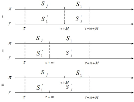
i. S1 =m,Sj =M,S10 =M,Sj0 =m, with probabilityp,
ii. S1 =M,Sj =m,S10 =m,Sj0 =M, with probabilityp,
iii. S1 =m,Sj =M,S10 =m,Sj0 =M, with probability 1−2p.
The coupling yields S10 ≤ Sj (and S1 ≤ Sj0) in all three cases. See Figure 3.4 for a visual
description of this coupling. In the first two cases all the arrival times to station 0 under
policies πandγ are identical. The system states for the two policies are identical after time
τ+m+M. Hence, policyγ can follow policyπ thereafter. By directly coupling the service
times of all jobs taken into service after time τ +m+M, we find thatDγ0(t) =Dπ
0(t) for
all t≥0.
In the third case, letS0 be the service time at station 0 for the job entering station 0 at
time τ +Sj under policy π and for the job entering station 0 at timeτ +S10 under policy
Figure 3.4: Sample path couplings for the parallel system.
1. 0 < S0 ≤m. We directly couple the service times of all jobs taken into service after
τ +m+M. The system states for the two policies will become identical after time
τ +m+M. Hence, policy γ can follow policy π after τ +m+M.
2. S0 > m. We directly couple the service times of all jobs taken into service after
τ +m+M. The system states for the two policies will become identical after time
τ +M +S0. However, policy γ can follow π after τ +m+M because same jobs or
more will be available to policy γ compared to policy π.
In both sub-cases, the problem can be analyzed in three intervals as below.
Dγ0(t) =
D0π(t), 0≤t < τ+m+S0,
D0π(t) + 1, τ+m+S0 ≤t < τ+M+S0,
D0π(t), t≥τ +M +S0.
Therefore,
D0γ(t)−Dπ0(t)≥0, for all t≥0,
and
T H0γ−T H0π = lim inf
t→∞
1
t[D
γ
We have shown that jobs at station 1 should be served ahead of the jobs at station jm if
jobs are available at both stations. Following the same argument iteratively, we can show
that a job at station 1 should be served ahead of the sequence of stations {j1, . . . , jm−1}.
In other words, if X1 ≤lrXj, j 6= 1, then jobs in station 1 should be prioritized in order to
maximize the long-run average throughput of the system.
Remarks. Theorem 3.3.2 says that we should give the highest priority to the service
station which has the shortest service times in likelihood ratio ordering among all service
stations. This follows the same intuition as in the series model where the optimal policy
pushes jobs towards the automated station as early as possible. Note that there is no
ordering condition required on the service times for the series system as opposed to the
parallel system. In Section 3.2.2, under preemptive policies and Markovian assumption, we
provide a complete characterization of the optimal policy. Under non-preemptive policies,
even though Theorem 3.3.2 only gives a partial characterization of the optimal policy for
K >2, we believe that a complete characterization should follow a similar intuition as we
state in the following conjecture.
Conjecture 3.3.1. If the service times at the service stations follow a likelihood ratio ordering, such as X1 ≤lr X2 ≤lr . . . ≤lr XK, then there exists an optimal policy which
maximizes the long-run average throughput and gives priority to the non-empty station with the smallest index at any decision epoch.
A numerical study is conducted in Section 3.3.4 to support Conjecture 3.3.1.
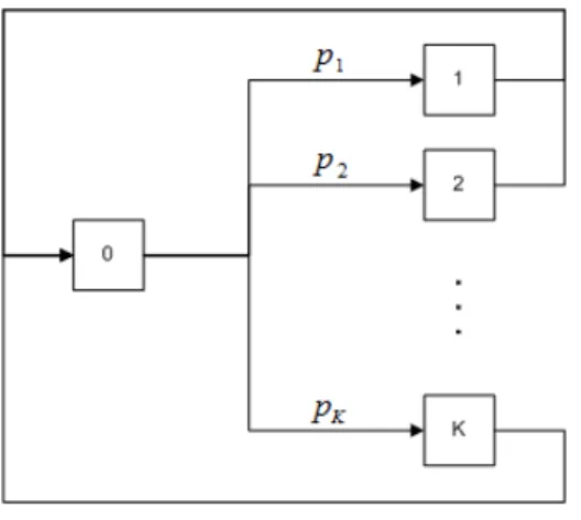
3.3.3 Two-Branch Three-Station System
In this subsection, we study a system with two branches and three service stations as shown
in Figure 3.5. Stations 2 and 3 are in series and parallel to station 1 as a whole. A job after
being served at station 0 will join station 1 with probabilityp1 or station 2 with probability
p2. This queueing system is motivated by the nurse staffing problem studied in Yankovic
and Green [35]. We consider this closed queueing system as a hospital ward, where a patient
seeks admission (station 3), then stays at a bed (station 0), then requests nursing service
(station 1) and returns back to his/her bed after receiving service (this process may repeat
comes to the ward immediately after a patient is discharged. We defineXi to be the random
variable denoting the i.i.d. service time at station i for i = 1,2,3. We provide a partial
Figure 3.5: A closed queueing system with an automated station and three service stations.
characterization of the optimal policy that maximizes the long-run average throughput of
the system in Theorem 3.3.3.
Theorem 3.3.3. If X1[X3]≤lr X3[X1], then there exists an optimal policy that gives the highest priority to station 1[3].
Theorem 3.3.3 partically characterizes the optimal policy: the faster station between
the two stations which directly connect to the entry of the automated station should be
prioritized, if the service times at these two stations are ordered according to likelihood
ratio ordering.
Proof of Theorem 3.3.3. We show that ifX1≤lrX3, then there exists an optimal policy
that gives the highest priority to station 1. The proof that an optimal policy gives the highest
priority to station 3 if X3 ≤lrX1 is similar.
Suppose policyπ is a policy under which there exists at least one decision epoch where
the highest priority is not given to station 1. Specifically, let ε be the first time policy π
does not give priority to station 1 even if there is a job in station 1. Suppose {j1, . . . , jm}
(j1, . . . , jm∈ {2,3}) gives the sequence of stations that the server visits after timeεbefore
it visits station 1 under policyπ. We will next construct a new policyγ which serves station
1 right before it serves the last job at station jm.
Let τ be the time under policy π that the server starts to work on a job at station 2
with service time S2 right before it moves to station 1. Then after completing serving this
job, the server immediately switches to station 1 to serve a job there with service time S1.
We construct the new policy γ as follows: γ followsπ during [0, τ) and then serves a job at
station 1 with service time S10, switches to station 2, and serves a job with service time S20.
We directly couple the service times of all jobs taken into service during [0,∞), which
yields S10 = S1 and S20 = S2. Let S0 be the service time at station 0 for the job entering
station 0 at timeτ+S2+S1under policyπ and for the job entering station 0 at timeτ+S10
under policy γ. γ followsπ during [τ +S1+S2,∞). This is possible because same jobs or
more are available to policyγ compared to policyπ. The system states for the two policies
will become identical after time τ +S2+S1 +S0. The problem can be analyzed in three
intervals as follows:
D0γ(t) =
Dπ0(t), 0≤t < τ+S10 +S0,
Dπ0(t) + 1, τ +S10 +S0 ≤t < τ+S2+S1+S0,
Dπ0(t), t≥τ+S2+S1+S0.
Therefore,
T H0γ(t)−T H0π(t) = lim inf
t→∞
1
t[D
γ
0(t)−D0π(t)]≥0, for all t≥0.
Case 2. (jm = 3)
Let τ be the time under policy π that the server starts to work on a job at station 3
with service time S3 before it moves to station 1. Then after completing serving this job,
the server immediately switches to station 1 to serve a job there with service time S1. We
construct a new policyγ as follows: γ followsπduring [0, τ) and then serves a job at station
1 with service time S10, switches to station 3 and serves a job with service timeS30.
We directly couple the service times of all jobs taken into service during [0, τ) and we
cross coupleS1,S3,S10,S30 as in the proof of Theorem 3.3.2 by first generating the minimum
and maximum of S1 and S3, namely m and M, respectively, conditioning on their values
and using these values in both policies. We need to consider three couplings:
i. S1 =m,S3=M,S10 =M,S30 =m,