Assets with possibly negative dividends

Munich Personal RePEc Archive

Assets with possibly negative dividends

Pham, Ngoc-Sang

Montpellier Business School, Montpellier Research in Management

7 April 2017

Online at

https://mpra.ub.uni-muenchen.de/78193/

Assets with possibly negative dividends

Ngoc-Sang PHAM

Montpellier Business School, France

April 7, 2017

Abstract

The paper introduces assets whose dividends can take any value (positive, negative or zero) in a dynamic general equilibrium model with financial market imperfections. We investigate the interplay between the asset markets and the production sector. The behavior of asset price and value is also studied.

Keywords: Infinite-horizon, general equilibrium, productivity, asset price, negative dividend

JEL Classification Numbers: D5, D90, E44, G12.

1

Introduction

The standard literature of asset pricing (Lucas,1978;Ljungqvist and Sargent,2012;

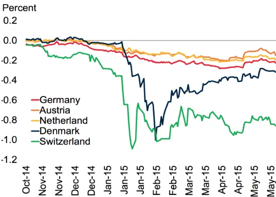
Asparouhova et al., 2016) considers that dividends of assets are positive. However, recently some central banks and governments issue assets with negative nominal interest rates (see Figures1,2below). Such these assets may have interpretation: once we buy an asset (money, for example), we will (1) be able to resell it, and (2) have to pay an amount (instead of receiving an amount as in the case of positive dividend). Motivated by this fact, our paper investigates the behavior of prices and values of assets whose dividends (or yields) may take any value (negative, positive or zero), and the interplay between the asset markets and the production sector.

To do so, we build an infinite-horizon general equilibrium model with a production sector and an imperfect financial market. There are a finite number of heterogeneous consumers and one representative firm (without market power). Consumers have two choices for investing: buy physical capital and/or buy a long-lived asset (whose initial supply is exogenous and positive) which brings dividends in the future (similar to the Lucas tree). The novelty is that asset dividend at each period may be positive, negative or zero.

Without the positivity of asset dividends, it is not trivial that asset prices are positive because it is possible that nobody buys this asset; in such a case, issuing

Figure 1: Policy rate on excess reserves, percent

Figure 2: Two-year government bond yields

Source: The World Bank, Global Economic Prospects, June 2015.

assets with negative dividend has no effect on the economy. Hence, we may interpret that one can run negative dividend policy if there exists an equilibrium where asset prices are positive at all dates.

We also prove that when asset dividends are negative at any period, there is no equilibrium with positive asset prices and borrowing constraints are not binding. We then provide examples where agents cannot borrow and asset dividends are negative at any date but asset prices are positive. Let us explain the intuition of this example where we assume that there is a fluctuation on endowments, which in turn creates a fluctuation on agents’ income. Consider a date: Agents, who have low endowment at the next date and cannot borrow, have to transfer their wealth from the present date to the next period, hence they accept to buy financial asset in the present date with positive prices even this asset brings negative dividends in the future. The same argument is applied for other dates and agents. Therefore, asset prices are positive at all periods. This result is stronger than the existence of fiat money, i.e., asset without dividend has positive price (Bewley, 1980; Tirole, 1985; Pascoa et al., 2011), and the existence of rational bubbles, i.e., the asset price is higher than the present value of future dividends (Santos and Woodford,1997;Le Van and Pham,2016), in the general equilibrium context.

Our second contribution is to identify conditions under which we should run negative dividend policy, i.e., we study the optimal distribution of dividends, given that the objective is the welfare. We find out that, when the productivity in the future is high enough, the government should issue an asset in the present, which will have negative dividend in the future. This action will provide investment for production sector, which will bring a high return because the productivity in the future is high. This suggests that while a central bank encourages people to invest by reducing interest rates (ECB,

2014), it is important for the economy to stimulate investments in R&D in order to improve the productivity in the future. Moreover, our analyses indicate that when the aggregate resource of the economy is low today, dividend at this date should be positive because asset dividend can provide financial support for the purchase of the physical capital, and then increase investment.

The last set of our contribution concerns the behavior of asset price and value. Let us denote qt and ξt the equilibrium asset price (in terms of consumption good) and

asset dividend at date t. Given that the asset supply is positive at any date, we have, as in Santos and Woodford (1997), so-called no-arbitrage condition

qt=γt+1(qt+1+ξt+1) (1)

where γt+1 is the endogenous discount factor of the economy from date t tot+ 1. By

iterating (1), we get the following decomposition

q0 =

XT

t=1

Qtξt

+QTqT (2)

where Qt ≡γ1· · ·γt is the endogenous discount factor of the economy from date 0 to

t.

In the standard theory,1 _ξ

t is assumed to be positive for any t. So, PTt=1Qtξt

is increasing in T, which implies that the discounted asset value QTqT decreasingly

converges to some value. When QTqT converges to zero, we can compute the asset

1_{SeeTirole(1982),Kocherlakota (1992), Santos and Woodford(1997),Le Van and Pham (2016)}

price by q0 = P∞t=1Qtξt; this kind of equilibrium is referred to no-bubble equilibrium

(Tirole, 1982; Kocherlakota, 1992; Santos and Woodford, 1997; Le Van and Pham,

2016).

We point out, by some examples, that when asset dividends (ξt) may be negative,

the sum PT

t=1Qtξt may diverge, and the discounted asset value QTqT may diverge or

converge to any value (even converge to infinity). Our examples are not trivial because

PT

t=1Qtξt converges to q0 if intertemporal marginal rates of substitution of agents are

the same or borrowing constraints are never binding (or without financial frictions). We also show that asset prices (qt) may fluctuate over time. Interestingly, there are

some cases where asset prices are zero at infinitely many dates and positive at other dates. These findings show how hard is the searching for a robust result on prices and values of assets whose dividends may be negative.

The remainder of the paper is organized as follows. Section 2 introduces our framework and presents some basic properties of equilibria. Section3provides analyses of equilibrium with positive asset prices by studying the interaction between asset market and production sector. In Section4, we investigate asset valuation and provide some examples illustrating and complementing our theoretical results. Section5concludes. Technical proofs are gathered in Appendix A.

2

Framework

Our model is based on Lucas (1978), Santos and Woodford (1997) and Le Van and Pham (2016). The novelty is that we do not require the positivity of dividends. In additional, different from Lucas (1978),Santos and Woodford(1997), we introduce capital accumulation. However, for simplicity, we assume that consumers are prevented from borrowing.

Time is discrete and runs from 0 to ∞. There are a finite number of households. Let us denoteI ≡ {1,2,· · · , m} the set of households.

Consumption good. There is a single consumption good at each date. At period

t, the price of consumption good is denoted by pt and agent i consumes ci,t units of

consumption good.

Physical capital. Let us denotertthe capital return at datetand δthe depreciation

rate, ki,t+1 the quantity of physical capital bought by agent i at datet.

Financial asset. At period t, if agent i buys ai,t units of financial asset with price

qt, she will receive ξt+1 units of consumption good as dividend and she will be able

to resell ai,t units of financial asset with price qt+1. Note that ξt may take any value

(negative, positive or zero). Whenξt= 0 for any t, the asset becomes fiat money as in

Bewley (1980), Pascoa et al. (2011) or pure bubble asset as in Tirole (1985), Hirano and Yanagawa (2017). When ξt > 0 for any t, we recover the Lucas’ tree in Lucas

(1978), or security in Santos and Woodford (1997) or stock in Kocherlakota(1992). Each household i takes the sequence of prices (p, q, r) = (pt, qt, rt)∞t=0 as given and

chooses allocation sequences (ci,t, ki,t+1, ai,t)∞t=0 to maximize her intertemporal utility.

The utility maximization problem of agent i is the following:

(Pi(p, q, r)) : max

(ci,t,ki,t+1,ai,t)∞t=0

∞ X

t=0

βitui(ci,t)

subject to

ki,t+1 ≥0, ai,t ≥0, (4)

pt(ci,t+ki,t+1−(1−δ)ki,t) +qtai,t ≤rtki,t+ (qt+ptξt)ai,t−1+ptei,t+θtiπt, (5)

where ei ≡ (ei,t) is the sequence of endowment of agent i while πt is the profit of the

firm at datet(see below). (θi

t)mi=1 is the share of profit at datet. θi ≡(θit)tis exogenous,

θi

t ≥0 for alli and

Pm

i=1θit= 1.

For each period t, there is a representative firm which takes prices (pt, rt) as given

and maximizes its profit by choosing physical capital amountKt.

(P(pt, rt)) : πt ≡max Kt≥0

ptF(Kt)−rtKt

(6)

Denote E the economy which is characterized by a list

(ui, βi, ei, ki,0, ai,−1, θi)mi=1, F, δ,(ξt)∞t=0

.

Definition 1. Consider the economy E. A sequence of prices and quantities

pt, qt, rt,(ci,t, ki,t+1, ai,t)mi=1, Kt

∞

t=0 is an equilibrium of the economy E if the following conditions are satisfied:

(i) Price positivity: pt>0, rt >0 and qt ≥0 for t≥0.

(ii) Market clearing: at each t ≥0,

X

i∈I

(ci,t +ki,t+1−(1−δ)ki,t) =et+F(Kt) +ξt

X

i∈I

ai,t−1 (7)

Kt =

X

i∈I

ki,t, (8)

X

i∈I

(ai,t−ai,t−1)≤0, qt

X

i∈I

(ai,t−ai,t−1) = 0 (9)

where et ≡Pi∈Iei,t is the aggregate endowment of the economy.

(iii) Optimal allocation plan: for eachi, (ci,t, ki,t+1, ai,t)∞t=0 is a solution of the problem

(Pi(p, q, r)).

(iv) Optimal production plan: for eacht≥0,Ktis a solution of the problem(P(pt, rt)).

Comments. In this definition, we do not require that qt > 0 for any t. The

asset’s market clearing condition (9) is in the spirit ofArrow and Debreu (1954), and

P

i∈I(ai,t−ai,t−1) = 0 if price qt > 0. As we will mention below, in some cases where

asset dividends are not positive, it is not easy to find out an equilibrium with qt > 0

for anyt. In condition (7), the termξtPi∈Iai,t−1 will be ξtifPi∈Iai,t−1 = 1. However,

when nobody buys asset, we have P

i∈Iai,t−1 = 0.

Standard assumptions are required in our paper.

Assumption (H1): ui is in C1, u′i(0) = +∞, and ui is strictly increasing, concave.

Assumption (H2): F(·) is inC1_{, strictly increasing, concave, F(0) = 0.}

Assumption (H3): At initial period 0, ki,0, ai,−1 ≥ 0, and (ki,0, ai,−1) 6= (0,0) for

i= 1, . . . , m. Moreover, we assume that Pm

Definition 2. Given (ξt), we say that a positive sequence of consumption and capital

(Ct, Kt) is feasible if Ct+Kt+1 ≤et+F(Kt) + (1−δ)Kt+ξt for any t.

Let (Dt) be defined by

D0 ≡ e0 +F(K0) + (1−δ)K0+max(0, ξ0), (10)

Dt ≡ et+F(Dt−1) + (1−δ)Dt−1 +max(0, ξt) ∀t≥0. (11)

We see that Dt is exogenous and depends on the function F and K0, δ, ξ1, . . . , ξt.

Moreover, Ct+Kt+1 ≤Dt for every t≥0. This leads to the following result.

Lemma 1 (the boundedness of consumption and capital stocks). Consider a feasible path (Ct, Kt). We have

1. Capital and consumption are in a compact set for the product topology.

2. Moreover, they are uniformly bounded if (et)t and (ξt)t are uniformly bounded

from above and there exists x0 such that F(x) + (1−δ)x+ supt(et+ξt)≤x for

every x≥x0.

One can prove that conditions in point 2 are satisfied if supt(et+ξt) < ∞ and

F′_{(∞)< δ.}

The following assumption ensures that utility of each agent is finite.

Assumption (H4): For each agent i,

∞

X

t=0

β_itui(Dt(F, δ, K0, ξ0, . . . , ξt))<∞. (12)

Price normalization. Since the utility function ui is strictly increasing, at any

equilibrium (if it exists),ptmust be positive for anyt. So, without loss of generality, we

can normalize by settingpt= 1 for anyt. In this case, we also call

qt, rt,(ci,t, ki,t+1, ai,t)mi=1, Kt

t

equilibrium.

2.1

Basis properties

We provide a necessary and sufficient condition to verify that a list of prices and allocations is an equilibrium.

Lemma 2. qt, rt,(ci,t, ki,t+1, ai,t)mi=1, Kt

t is an equilibrium if and only if there exist

sequences (σi,t, νi,t)i,t such that the following conditions are satisfied, for any i and for

any t,

(i) ci,t >0, ki,t+1 >0, ai,t >0, σi,t >0, νi,t >0, Kt>0, qt ≥0, rt>0.

(ii) First order conditions:

1

rt+1+ 1−δ

= βiu

′

i(ci,t+1)

u′

i(ci,t)

+σi,t, σi,tki,t+1 = 0

qt

qt+1+ξt+1

= βiu

′

i(ci,t+1)

u′

i(ci,t)

(iii) Transversality condition:

lim

t→∞β

t iu

′

i(ci,t)(ki,t+1+qtai,t) = 0. (13)

(iv) F(Kt)−rtKt= max{F(k)−rtk :k >0}.

(v) ci,t +ki,t+1−(1−δ)ki,t+qtai,t =rtki,t+ (qt+ξt)ai,t−1+θitπt+ei,t

where πt =F(Kt)−rtKt.

(vi) Kt=Pi∈Iki,t

(vii) P

i∈I(ai,t−ai,t−1)≤0, and

P

i∈I(ai,t −ai,t−1) = 0 if qt >0.

Transversality condition (13) which is not trivial can be proved by adapting the argument in the proof of Theorem 1 in Kamihigashi (2002). The proof of Lemma

2 is left to the reader. The readers are referred to Araujo et al. (2002), Pascoa et al. (2011), Bosi et al. (2017) for similar conditions in economies with uncertainty, incomplete markets and collateral constraints.

Remark 1. Consider a finite T-period economy. If ξt ≤ 0 for any t ≤ T, there does

not exist an equilibrium with qt >0 for any t≤T −1.

Let us denote, for each t≥0, γi,t+1 (respectively,Qi,t) the agent i’s discount factor

from datet to datet+ 1 (respectively, from initial date to date t) as follows.

γi,t+1 ≡

βiu′i(ci,t+1)

u′

i(ci,t)

, Qi,0 = 1, Qi,t ≡γi,t· · ·γit. (14)

We also define γt+1 the discount factor of the economy from date t tot+ 1 andQt

the discount factor of the economy from date 0 tot

γt+1 ≡max

i

β

iu′i(ci,t+1)

u′

i(ci,t)

, Q0 = 1, Qt≡γ1· · ·γt. (15)

According to point (iii) of Lemma 2, we have so-called non-arbitrage inequalities.

Lemma 3. At equilibrium, we have, for each t,

qt≥γt+1(qt+1+ξt+1) with equality if

X

i

ai,t >0 (16)

1≥γt+1(rt+1+ 1−δ) with equality if Kt+1 >0 (17)

Note that Qtki,t+1 = (1−δ+rt+1)Qt+1ki,t+1 for any t and for any i.

In the remainder of the paper, we will focus on equilibria where all prices are positive, i.e. qt>0 for anyt. In this case, we have Piai,t = 1 for any t, and therefore

3

Negative dividend and production

The asset in our framework can be interpreted as an asset issued by the government who can choose negative dividends at some or all dates. However, such an action has no effect on the economy if the asset price is zero or nobody buys the asset. This motivates us to introduce the following notion.

Definition 3. We say that the government can run negative dividend policy if there exists an equilibrium with qt>0 for any t.

The aim of this section is to find out conditions under which the government can run negative dividend policy.

3.1

Can we run negative dividend policy?

First, we consider the case where asset dividend at only one date may be negative. We have the following result.

Proposition 1. Assume that Assumptions (H1)-(H4) hold and ui(0) = 0 for any i.

Consider a date s∗ _{≥0. Assume that ξ}

t≥0 for anyt 6=s∗, and there is an infinite

sequence (ξtn)n such that ξtn >0 for anyt. Then, there exists ξ >¯ 0 such that: for any

ξs∗ ≥ −ξ¯, there exists an equilibrium with q_t>0 for any t.

Proof. See Appendix A.1.

According to this result, the existence of equilibrium is ensured if asset dividend at some date is negative but not far from zero (in the sense thatBi,t >0). In particular,

we recover the existence result in Le Van and Pham (2016) for the case ξt >0 ∀t.

In what follows, we will consider more general cases where dividends at any date may be negative. We start by pointing out the behavior of asset price and value in the very long run.

Lemma 4. Assume that 0 < lim inft→∞ξt ≤ lim supt→∞ξt < +∞,2 and conditions

in point 2 of Lemma 1 hold. Then, for any equilibrium, we have lim

t→∞Qtqt = 0 and

qs=P∞t=s+1Qtξt/Qs for each s ≥0. Consequently, qt>0 when t is high enough.

Proof. See Appendix A.2.

Lemma 4 provides a sufficient condition under which the present value P∞

t=1Qtξt

converges. Moreover, the equilibrium price at any date is equal to the present value of future dividends, which is equivalent to the fact that the discounted value of asset will converge to zero, i.e. limt→∞Qtqt= 0. Lemma4also gives a sufficient condition under

which asset prices are positive in the very long run. Notice that under assumptions in Lemma 4, aggregate consumption and capital stocks are uniformly bounded from above.

Some interesting consequences of Lemma 4 should be mentioned.

Corollary 1. Assume that 0 <lim inf

t→∞ ξt ≤lim sup_t→∞ ξt < +∞, and conditions in point

2 of Lemma 1 hold. Let us consider a date s ≥ 0 such that ξs < 0. Consider an

equilibrium.

1. If qs−1 >0, then P∞t=s+1Qtξt> Qs|ξs|>0.

2. If Kt>0 for any t≥0, then we have

∞

P

t=s+1(F

′_{(0) + 1−δ)}t−s_|ξ

t| ≥ |ξs|>0.

Point 1 in Corollary1indicates that when dividend at some date, says, is negative, the asset price at date (s−1) is positive only if the present value of dividends at date

s is strictly higher than the absolute discounted value of asset at this date. Note that when conditions 0 < lim inft→∞ξt ≤ lim supt→∞ξt < +∞ are violated,

P∞

t≥s+1Qtξt

may be lower than Qs|ξs|; this property will be readdressed in Section 4.2. Point 2

in Corollary 1 complements Proposition 1 by providing an upper bound of −ξs when

ξs<0. This upper bound depends on productivity and future dividends.

Using transversality condition (13) in Lemma2, we have the following result showing the role of intertemporal marginal rates of substitutionsγi,t+1 ≡βiu′i(ci,t+1)/u′i(ci,t).

Proposition 2 (role of agents’ heterogeneity).

1. If there is a date t0 such that γi,t = γt for any t > t0 and for any i, then

limt→∞Qtqt= 0 and Qtqt=P∞s=t+1Qsξs

2. Consequently, ifξt≤0for anyt, then there is no equilibrium with positive prices

such that γi,t =γt for any t, i or ai,t >0 for any t, i.

Proof. See Appendix A.3.

According to Proposition2, when all dividends are negative, there is no equilibrium with positive prices in which the intertemporal marginal rates of substitutions are the same at any period (this happens if agents are identical). The intuition is the following: when the intertemporal marginal rates of substitutions are the same, agents’ investment behavior are similar; in such a case, nobody buys assets with negative dividends. So, asset prices are zero at any date.

If borrowing constraint ai,t ≥0 is not binding for any i, we have γi,t+1 =γt+1. By

the way, point 2 of Proposition2indicates the role of borrowing constraints: When all dividends are negative, at each equilibrium with positive prices, there exist an agent

i and an infinite sequence (tn)n≥1 such that ai,tn = 0 for any n ≥ 1. Section 4.2 will

provide some examples whereξt≤0 for anyt, asset prices are positive, and borrowing

constraints are frequently binding.

We now analyze the role of productivity. We prepare our exposition by an intermediate step.

Lemma 5. If there exists an equilibrium with qt>0∀t, then ξt is bounded from below

by an exogenous parameter: ξt ≥ −et −F(Dt−1)−(1−δ)Dt−1 for any t, where the sequence (Dt)t is defined by (10) and (11).

Proof. If an equilibrium exists, we have 0≤Ct+Kt+1 ≤F(Kt) + (1−δ)Kt+ξt. By

Lemma 5 indicates that the existence of equilibrium with positive prices (qt > 0

for any t) requires that asset dividends must be bounded from below by exogenous parameters. This leads to the following result.

Proposition 3 (role of productivity). Assume that et= 0 for any t.

1. Assume that there exists d such that ξt ≤ −d < 0 for any t. If F′(0) < δ and

F(0) = 0, then there is no equilibrium with qt >0 for any t.

2. (collapse). Assume that ξt ≤0for any t, F′(0)< δ and F(0) = 0. If there exists

an equilibrium with qt>0 for any t, then lim

t→∞ξt= 0 and tlim→∞Kt= 0.

Proof. See Appendix A.4.

The first point shows that when dividends are negative and bounded above by a negative constant, there is no equilibrium with positive prices if the productivity is low. Point 2 of Proposition 3 indicates that when dividends are negative and productivity is low, an equilibrium exists only if dividends tend to zero and in this case the economy will collapse (aggregate consumption stocks converge to zero).

Let us explain the economic intuition of our result. When asset prices are positive at any date, there are always some agents who buy this asset. At any date, if one agent buys asset whose future dividends are negative, she will be able to resell this asset but have to pay an amount at the same time. In the aggregate level, the economy has to finance an amount (corresponding to negative dividends) at any date, which is bounded away from zero (−ξt > d > 0). However, when productivity is very low (F′(0) < δ),

the production level decreases in time and tends to zero, the economy collapses. By consequence, there will be some period when the resource of the economy will not be enough to cover negative dividends. Therefore, asset prices cannot be positive.

Propositions1and3suggest that negative dividend policies may be sustained only if (1) the production sector is strong enough (high productivity) and (2) dividends are not so low.

3.2

Should we run negative dividend policy? Optimal dividend

distribution

In this section, we wonder whether we should run negative dividend policies or not. It is reasonable to assume that the government chooses dividends in order to maximize the welfare of agents in the decentralized economy.

Since we are interested in the role of productivity, we allow for non-stationary production functions: the production function at datet is given by Ft(K) =AtF(K),

whereF is strictly increasing, strictly concave, F(0) = 0, F′_{(0) =∞, F(∞) = ∞, and}

At≥0 represents the total-factor productivity (TFP) of the economy..

For the sake of tractability, we assume that there is one representative household with instantaneous utility function u, the rate of time preference β ∈ (0,1), and non-negative endowments (et). The agent’s allocation is denoted by (ct, kt+1, at)t≥0.

and therefore the welfare function which depends on (ξt) is given by

W((ξt)t≥0)≡ max (ct,kt+1)t≥0

∞ X

t=0

βtu(ct)

(19)

subject to: kt+1 ≥0, ct+kt+1 ≤Gt(kt) +et+ξt (20)

where Gt(k) = (1−δ)k+Ft(k).

By the concavity of u and Gt, one can prove that the function W((ξ)t) is concave

in (ξt).

Assume that the government’s problem is to maximize the welfare function by choosing the sequence of dividend (ξt) subject to

ξt ≥ −bt ∀t≥0, and

∞

X

t=0

ξt ≤B, (21)

where B ≥ 0, bt > 0 for any t. Within this setup, the government, having an

endowment B ≥ 0 units of consumption good, has to distribute dividends across periods. The government can choose negative dividend at each date but there is a lower bound bt.

To find out the properties of the government’s optimal choice (ξt), we will study

the following problem.

(P W) : max

(ct,kt+,ξt)t

∞ X

t=0

βtu(ct)

(22)

subject to: kt+1 ≥0, (23)

ct+kt+1 ≤Gt(kt) +et+ξt (24)

ξt≥ −bt (25)

X

t

ξt ≤B. (26)

We assume that (bt) is not so high so that the set of choices of the problem (PW)

is not empty. Therefore, the problem (PW) has a solution.

Notice that the non-standard optimal growth problem (PW) is non-stationary and has no closed-form solution. Moreover, it is not easy to find out global property of the solution. Here, we can provide some qualitative analysis. The following result shows the role of productivity.

Proposition 4. Let assumptions in this section be satisfied andu(∞) =∞, u′_{(∞) = 0.}

Fix a datetand all parameters, exceptAt. Then, there existsA¯tsuch that each solution

of the problem (PW) satisfies: ξt=−bt <0 for any At ≥A¯t.

Proof. See Appendix A.5.

The intuition of Proposition 4is the following. Let us interpret date (t−1) as the present and date t as the future. When the productivity in the future is high enough, the government should issue an asset in the present which will have negative dividend in the future. This action provides investment for the production sector, which will bring a high return because the productivity in the future is high.

Corollary 2. Let assumptions in this section be satisfied and u(∞) =∞, u′_{(∞) = 0.}

Assume that the government can only choose ξ0, ξ1 such that ξ0 ≥ −b0, ξ1 ≥ −b1 and

ξ0+ξ1 ≤D where D >0.

Fix all parameters, except A1. There exists A¯1 such that at optimal, ξ1 =−b1 <0 and ξ0 =D+b1 >0 for any A1 ≥A¯1.

This result complements Proposition4. It indicates the moments when the government should choose positive and negative dividends. Dividend should be positive today if the productivity in the future is high enough because in this case asset dividend can provide financial support for the purchase of the physical capital, and then increase investment.

3.2.1 A closed-form solution

In order to see more clearly economic intuitions, this section provides an example where we can find a closed-form solution. Consider a two-period model. Assume that

u(c) = ln(c). Assume also that δ = 1, Ft(k) = Atk1/2 for t = 0,1. The welfare

function, which depends on ξ0, ξ1, is defined by

W(ξ0, ξ1)≡ max (c0,k1,c1)

ln(c0) +βln(c1)

subject to: k1 ≥0,

c0+k1 ≤A0k01/2+e0+ξ0

c1 ≤A1k11/2+e1+ξ1.

The standard Euler equation u′_(c

0) =βu′(c1)1₂A1k

−1/2

1 implies that

(1 +β1

2)A1k1+ (e1+D−ξ0)k

1/2 1 −β

1

2A1(A0k

1/2

0 +e0+ξ0) = 0.

Some comments should be mentioned here.

• It is easy to see that when ξ0 increases, k1 increases.

• Sinceξ0+ξ1 is constant, if we decrease ξ1, thenξ0 and so k1 increases, therefore

the interest rate on the capital marketr1 = 1₂A1k

−1/2

1 decreases. This corresponds

to what the banks wanted to do: decrease the interest rate to enhance investment (see for example ECB (2014)).

When ξ0 increases, the aggregate at initial date (A0k01/2+e0+ξ0) and production

at next date (A1k11/2) increase but ξ1 decreases. So, the consumption at next date

(A1k11/2 +e1 +ξ1) may decrease, and therefore it is not trivial that the welfare is an

increasing function of ξ0. The following example gives a closed-form solution for the

optimal level of dividend distribution (ξ0, ξ1).

Then, the government’s solution is given by

ξ0 = ¯ξ0 ≡

(2 +β)A2 1+ 4

e1+B−β(A0k01/2+e0)

4(1 +β) (27)

ξ0+ξ1 =B (28)

Here, we explicitly assume that ξ¯0 ∈ [−b0, B]. We also need ξ¯1 ≡ B −ξ¯0 > 0 in order to ensure that q0 >0.3

Proof. See Appendix A.6.

According to (27), the optimal level of ξ0 may be negative or positive. It depends

positively onA1, e1 but negatively onA0, k0, e0. Moreover, it depends positively on the

total amount B of dividends. This result complements the findings in Proposition 4

and Corollary 2.

It is easy to see that the optimal level ofξ0is negative if the endowment at the initial

period A0k01/2+e0 is high enough. It means that the country is rich enough (high k0

ande0) or/and has high productivity (highA0). This finding is totally consistent with

empirical data mentioned in the introduction: only rich countries experience negative nominal interest rates. Moreover, our analyses in this example and Proposition 4

suggest that while a central bank encourages people to invest by reducing interest rates (ECB, 2014), it is important for the economy to stimulate investments in R&D in order to improve the productivity in the future.

The optimal level of ξ0 is positive if

• the productivity at the second periodA1 is high enough, as in this situation, the

higher the investment at the initial period, the higher the level of output at the second period. This is consistent with Corollary 2;

• or/and endowment at the second period e1 is high enough. Indeed, when the

economy has enough endowment at the second period, positive dividend at the initial period may benefit consumption at this period and then the total welfare.

4

Asset valuation

In this section, we investigate the asset valuation by developing the standard asset pricing for the case where dividends may be negative. By iterating (18) we have the following decomposition

q0 =

_XT

t=1

Qtξt

+QTqT ∀T ≥1. (29)

The price q0, the value of one unit of asset at date 0, equals the sum of two terms:

The first F VT

0 ≡

PT

t=1Qtξt is the sum of discounted values of dividends until date T,

3

and the second one QTqT, called re-sold term, is the discounted value of one unit of

asset at dateT. We also have a similar decomposition for the asset price at date t.

Qtqt=

XT

s=t+1

Qsξs

+QTqT ∀T > t. (30)

Consider the Lucas tree with the sequence of positive dividends (ξt). The standard

literature of asset pricing in infinite-horizon models (Tirole, 1982;Kocherlakota,1992;

Santos and Woodford, 1997; Le Van and Pham, 2016) defines the fundamental value of this asset byF V ≡P∞

t=1Qtξt and the bubble of this asset as the difference between

the equilibrium price and the fundamental value q0 −F V; in some mild situations,

there is no bubble and we can compute the asset price byq0 =F V.

This standard approach is suitable for assets with positive dividends becausePT

t=1Qtξt

is increasing in T and so converges if ξt ≥ 0 for any t. However when we consider

assets whose dividends may be negative, there is a room for the divergence of the series P

t≥1Qtξt. Hence, the standard approach cannot be applied.

4.1

Asset value at infinity

A natural question concerns the behavior of the discounted value of one unit of the asset in the long run, i.e., limt→Qtqt. This makes sense because in the case where

limt→Qtqt = 0, we can compute the asset price byq0 =P∞t=1Qtξt. When dividends are

positive, thanks to the decomposition (29),Qtqtis bounded and decreasingly converges

to some value (which is referred to the bubble of asset price bubble). However, if dividends may be negative, the story becomes more complicated. Let us start by considering two particular cases.

Proposition 5 (Value and price of asset).

1. (Montrucchio, 2004; Le Van and Pham, 2014). Assume that ξt >0 for anyt. At

any equilibrium, both PT

s=t+1Qsξs and QTqT converge, and

Qsqt=

X∞

s=t+1

Qsξs

+ lim

T→∞QTqT.

Moreover, we have (i)(QTqT)is decreasing in timeT, and (ii)limT→∞QTqT >0

if and only if P∞

t=1(ξt/qt)<∞.

2. Assume that ξt ≤ 0 for any t. At any equilibrium with qt > 0 for any t, both

PT

s=t+1Qsξs and QTqT converge, and

Qtqt =

_X∞

s=t+1

Qsξs

+ lim

T→∞QTqT.

Moreover, we have

(i) (QTqT)T is increasing in time T,

(ii) lim

T→∞QTqT < ∞ if and only if Tlim→∞

T

Q

t=1(1 +

ξt

qt) > 0, which is equivalent to ∞

P

t=1

−ξt

qt+ξt

<+∞, and this implies that P∞

t=1

−ξt

Proof. See Appendix A.7.

In Proposition 5, we see thatQtqt converges because either ξt ≥0 ∀t or ξt≤0 ∀t.

However, in more general cases,Qtqt may diverge. This issue will be addressed in the

next section.

To understand the meaningful of Proposition 5’s point 2, let us observe the budget constraint of agent i at datet

ci,t+ki,t+1−(1−δ)ki,t+qtai,t ≤rtki,t+ (qt+ξt)ai,t−1 +ei,t+θtiπt.

We see that one unit of asset bought at date t−1 will give one unit of the same asset and ξt units of consumption good (i.e., (qt+ξt) units of consumption good) at

date t. When ξt < 0, the ratio _q−_t+ξ_ξt_t can be interpreted as the interest-to-value ratio

(proportion of interest to asset value) of asset at date t. By the way, point 2.ii shows that asset value at infinity is finite if and only if the sum (over time) of interest-value ratios is finite. This also implies that interest rate (in terms of asset), −ξt/qt, must

converge to zero.

4.2

Example: Positive asset prices with negative dividends

This section provides an example where the price of asset may be positive even its dividends are negative at all dates.

Fundamentals of the economy. In this section, we will work under the following setup. There are 2 consumersH andF with the same utility function and rate of time preference: ui(c) =ln(c), βi =β ∈(0,1) ∀i={H, F}. Their initial endowments are

respectively kH,0 = 0, aH,−1 = 0, kF,0 >0, aF,−1 = 1. Their endowments are given by

(eH_2t, eF₂) = (et,0), (eH2t+1, eF2t+1) = (0, et+1).

Assume that the production functions are given by F(K) =atK whereat ≥0 and

β(1−δ+at)≤1 for anyt. Note that πt= 0 for any t.

We also need P∞

s=1βtln(et)<∞ to ensure that consumers’ utilities are finite.

Computing equilibria. With the above setup, equilibria can be computed as follows. Allocations of the consumer H are given by

kH,2t = 0, aH,2t−1 = 0, kH,2t+1 =K2t+1, aH,2t = 1

cH,2t−1 = (1−δ+r2t−1)K2t−1+q2t−1+ξ2t−1, cH,2t =e2t−K2t+1−q2t

while allocations of the consumer F are

kF,2t =K2t, aF,2t= 1, kF,2t+1 = 0, aF,2t= 0

cF,2t−1 =e2t−1−K2t−q2t−1, cF,2t= (1−δ+r2t)K2t+q2t+ξ2t.

Prices and the aggregate capital are given by the following system: for any t,

pt= 1, rt =at, and

Kt+1+qt =

β

1 +βet (31)

qt+1+ξt+1 =qt(at+1+ 1−δ) (32)

By using Lemma 2, we can verify that this sequence of allocations and prices is an equilibrium. For short, we also call (Kt+1, qt)t≥0 equilibrium. It is easy to see that

Qt=

1

(1−δ+a1)· · ·(1−δ+at)

; Qtqt =q0−

t

X

s=1

Qsξs (34)

q0 ∈

0, βe0

1 +β

; 0≤q0−

t

X

s=1

ξs

(1−δ+a1)· · ·(1−δ+as)

< βet

1 +β ∀t (35)

Example 2 (Multiple equilibrium prices). Assume at =δ and et =e for any t, then

γt= 1 and Qt= 1 for any t. For each q0 such that

q0 ∈

0, βe

1 +β

, 0< q0−

t

X

s=1

ξs<

βe

1 +β ∀t, (36)

we determine

qt≡q0−

t

X

s=1

ξs, Kt+1 ≡

βe

1 +β −qt >0. (37)

It is easy to see that (Kt+1, qt)t≥0 is an equilibrium and qt>0 for any t.

In Example 2, we see that even when ξt is negative for any t, all asset prices

are positive. Let us explain the intuition of this fact. A fluctuation on wealth (or endowments) creates a fluctuation on agents’ income. In the odd periods (2t + 1), agent H has no endowment. She wants to smooth consumption over time but she cannot transfer her wealth from the future back to this date because of borrowing constraint. By consequence, she needs to transfer her wealth from date 2t to date 2t+ 1, hence she accepts to buy financial asset at date 2twith positive prices even this asset brings negative dividends in the future. The same argument is applied for the even periods and agent F. Therefore, asset prices are positive at any date.

This result is stronger than the existence of fiat money or of rational bubbles in the general equilibrium context. Indeed, Bewley (1980), Tirole (1985), Kocherlakota

(1992), Pascoa et al. (2011),Hirano and Yanagawa (2017) point out that the price of an asset without dividends (i.e., fiat money) may be positive.4 _{Santos and Woodford} (1997),Le Van and Pham (2016), Bosi et al. (2017) provide some examples where the asset price is higher than the sum of discounted values of asset dividends (which are always positive).

Remark 2. Lets ≥0. Take ξt = 0 for any t≥s andξs <0. In this case

∞

P

t=s+1Qtξt =

0<−ξs < Qsqs. This suggests that condition lim inf

t→∞ ξt >0 in Corollary 1 is essential

in order to ensure that P∞

t=s+1Qtξt> Qs|ξs|.

4_{This may happen in an OLG model (Tirole,1985) if the real interest rate of the economy without}

4.3

Fluctuations of asset price and (discounted) value

Given an equilibrium, the conventional view5 _{is that the discounted value of one} unit of the asset (i.e., (Qtqt)t) is bounded from above and converges. This property

holds because the existing literature only considers the case where dividends are always positive. In this section, we will investigate the behavior of (Qtqt) to know whether it

can diverge or converge when dividends may be negative.

Example 3. Consider again the example in Section 4.2 but we only requireat =δ for

anyt. It is easy to see that(Kt+1, qt)t≥0 determined by (31), (32), and (33), constitutes an equilibrium if

q0 ∈

0, βe0

1 +β

, 0≤q0−

t

X

s=1

ξs <

βet

1 +β ∀t (38)

Notice that under these conditions, we have Qt = 1 and Qtqt =qt=q0−Pts=1ξs.

Let us point out some consequences of Example 3.

1. Fluctuations of asset price and value. When we choose (ξt) such that (Pts=1ξs)t

diverges, then the sequence of asset prices (qt) diverges and so does (Qtqt).

In particular, we can choose q0 ∈

0, βe0

1+β

and (ξt) such that q0 −Pts=1ξs > 0

for any even t and q0 −Pts=1ξs = 0 for any odd t. Therefore, in general case,

asset priceqtmay be zero at infinitely many dates and it may also be positive at

infinitely many other dates.

2. Asset value converges to infinity. When we take (et) such that limt→∞et = ∞

and βet

1+β > βb0

1+β − t

P

s=1ξs,

6 _{we have that: Q}

tqt tends to infinity if and only if

P∞

s=1ξs = −∞. According to point 2 of Proposition 5, this is equivalent to

P

t≥1 _q0−(ξ1+ξ···t +ξt−1) =−∞.

5

Conclusion

When dividends may be negative, asset prices are positive only when the production sector is strong enough and dividends are not so low. Our analysis suggests that when the productivity in the future is high, issuing an asset in the present having negative dividends in the future may increase the welfare.

It is hard to find out robust behaviors of asset prices and values when dividends may be negative. The discounted value of one unit of asset Qtqt may fluctuate over

time. It may also converge to any positive value, even to infinity. Interestingly, asset prices may be positive even dividends are negative at all dates.

Acknowledgments

This paper is inspired by a conversation between Cuong Le Van and the author. The author would like to thank Cuong Le Van for his insightful discussions.

5

SeeTirole(1982,1985),Santos and Woodford(1997),Le Van and Pham(2016) among others.

6_{For example, takeξ}

A

Appendix: Formal proofs

A.1

Proof of Proposition

1

Let (Bi,t) be defined by

Bi,0 ≡(1−δ)ki,0+ξ0ai,−1, Bi,t ≡(1−δ)Bi,t−1+ξtai,t−1.

We will show that: if Bi,t >0 for any i, t then there exists an equilibrium withqt ≥0

andpt>0 for anyt. This can be done by adapting the argument inLe Van and Pham

(2016).

We have qt > 0 because there is an infinite sequence (ξtn)n such that ξtn > 0 for

any t

A.2

Proof of Lemma

4

By iterating (18) we have the following decomposition

q0 =

_XT

t=1

Qtξt

+QTqT ∀T ≥1 (A.1)

Qtqt=

XT

s=t+1

Qsξs

+QTqT ∀T > t. (A.2)

We see that there existsξ >0 andt0 > ssuch that ξt≥ξ for anyt ≥t0. So, when

T is high enough, the sequence (F VT

0 ≡

PT

t=1Qtξt)T >t0 is increasing in T. Moreover,

F VT

0 ≤q0 for any T. By consequence, F V0T converges to F V0 ≡ P∞t=1Qtξt < ∞ and

hence Qtqt converge. Since lim inft→∞ξt >0, we get that P∞t=1Qt <∞.

According to point 2 of Lemma1,et+F(Kt) is uniformly bounded from above. As a

result, we obtain that limT→∞QTki,T+1 = 0 for anyi, and so P∞t=1(et+F(Kt)Qt)<∞

because et is also uniformly bounded from above.

For each agent i, we rewrite her/his budget constraint at date t as follows

Qtci,t+Qtki,t+1+Qtqtai,t = Qt(rt+ 1−δ)ki,t+Qt(qt+ξt)ai,t−1+ (ei,t+θiπt)Qt.

By summing the budget constraints from t equals 0 to t, and use (17), (18), we get that

T X

t=0

Qtci,t

+QTki,T+1+QTqTai,T

= (r0 + 1−δ)ki,0+ (q0+ξ0)ai,−1+

T

X

t=0

(ei,t+θiπt)Qt<+∞

where the last inequality is from the fact that P∞

t=1

et+F(Kt)

Qt<∞.

We have QTqTai,T +QTki,T+1 ≥0, hence P∞t=0Qtci,t <+∞, and then (QTki,T+1+

QTqTai,T)T converges where T tends to infinity. Since limT→+∞QTki,T+1 = 0, the

If limT→+∞QTqT >0, then ai,T converges for any i. By consequence, there exists

i such that lim

t→+∞ai,t > 0. For such an agent, there existsT such that the ai,t >0 for

any t ≥T. Thus, Qt

QT =

Qi,t

Qi,T for any t ≥T. According to condition (13) in Lemma 2,

we have

lim

t→+∞Qtqtai,t =

QT

Qi,T

lim

t→∞Qi,tqtai,t = 0

which is a contradiction. We conclude thatQTqT converges to 0. Therefore, it is easy

to see that qt=P∞s=t+1Qsξs/Qt>0 for any t > t0.

A.3

Proof of Proposition

2

Point 1. Let an equilibrium such that γi,t = γt for any t > t0 and for any i.

According to point (iii) of Lemma 2, we have limt→∞Qt

qtai,t+ki,t+1

= 0 for any i. This implies that limt→∞Qtqt = limt→∞QtKt+1 = 0. By combining this with (A.2),

we obtainQtqt =

∞

P

s=t+1Qsξs.

Point 2 is a direct consequence of point 1.

A.4

Proof of Proposition

3

Proof of point (1). According to Lemma 5, we have F(Dt−1) +Dt−1 ≥ ξt ≥ d > 0

for any t. So, Dt is bounded away from zero.

By definition, we have

Dt=et+F(Dt−1) + (1−δ)Dt−1+ max(0, ξt)

=F(Dt−1) + (1−δ)Dt−1 <(F′(0) + 1−δ)Dt−1.

Since F′_{(0)< δ, we obtain that D}

t converges to zero, a contradiction.

Proof of point (2). By definition, we have Dt ≥ Ct+Kt+1, so both Ct and Kt+1

converge to zero.

Ifξtdoes not converge to zero, there existξ >0 and an infinite sequence (tn)n such

that ξtn ≤ −ξ for any n. Hence, F(Ktn) + (1−δ)Ktn ≥ −ξtn ≥ ξ > 0. So, Ktn is

bounded away from zero, a contradiction.

A.5

Proof of Proposition

4

By Lemma1and Assumption H4, the problem (PW) has a solution. Let (ct, kt+, ξt)t

be a solution of this problem. We have first order conditions

λt =βtu′(ct) (A.3)

λ =λt+µt, µt(ξt+bt) = 0 (A.4)

λt =λt+1G′t+1(kt+1) (A.5)

for any t, where λt, µt, λ are non-negative multipliers associated to constraints (24),

We fix a date t.

Suppose that ξt>−bt, thenµt= 0. We have

1 = λ

λ =

λt

λt+1+µt+1

≤ λt

λt+1

=G′

t+1(kt+1). (A.6)

We will claim that Gt(Kt) tends to infinity when At tends to infinity. Indeed,

suppose Gt(Kt) is bounded, then the sequence (ct)t is bounded and so is the welfare.

However, it is easy to see the the welfare tends to infinity when At tends to infinity

because u(∞) =F(∞) =∞.

We now prove that Kt+1 tends to infinity when At tends to infinity. Suppose that

Kt+1 is bounded, then limAt→∞ct=∞ (because ct+kt+1 =Gt(kt) +et+ξt). We see

that (ct+1) is bounded because Kt+1 is bounded. Hence u′(ct+1) and G′t+1(kt+1) are

bounded away from zero. By FOCs, we get that

1 = βu

′_(c

t+1)

u′_(c

t)

G′

t+1(kt+1).

Hence, u′_(c

t) is also bounded away from zero. We have a contradiction because

limAt→∞ct=∞and u

′_{(∞) = 0.}

Therefore, we have proved that Kt+1 tends to infinity when At tends to infinity.

This implies that lim

At→∞

G′

t+1(kt+1) = 1−δ < 1, a contradiction to (A.6). Finally, we

get ξt=−bt <0.

A.6

Proof of Example

1

It is easy to see that W(ξ0, D − ξ0) is differentiable. We have, by noting that

u′_(c

0) =βu′(c1)G′1(k1),

∂W ∂ξ0

=u′

(c0)−

∂k1

∂ξ0

u′

(c0)−βu′(c1) +βu′(c1)G′1(k1)

∂k1

∂ξ0

(A.7)

=u′

(c0)−βu′(c1) =βu′(c1)(G′1(k1)−1). (A.8)

We now compute G′

1(k1). Euler condition u′(c0) =βu′(c1)G′1(k1) implies that

A1k11/2+e1+ξ1 =β

1 2A1k

−1/2

1 (A0k10/2+e0+ξ0−k1).

Hence, (1 +β1₂)A1k1+ (e1+D−ξ0)k11/2−β1₂A1(A0k01/2+e0+ξ0). So, we can find

that

k11/2 =

−(e1+D−ξ0) +

q

(e1+D−ξ0)2+β(2 +β)A21(A0k01/2+e0+ξ0)

(2 +β)A1

. (A.9)

Thus, condition G′

1(k1)≥1 becomes 1

2A1(2 +β)A1

−(e1+D−ξ0) +

q

(e1+D−ξ0)2+β(2 +β)A21(A0k01/2+e0+ξ0)

≥1

⇔

1

2A1(2 +β)A1

e1+D−ξ0+

q

(e1+D−ξ0)2 +β(2 +β)A21(A0k10/2+e0+ξ0)

β(2 +β)A2

1(A0k10/2+e0+ξ0)

This inequality is equivalent to

q

(e1+D−ξ0)2+β(2 +β)A21(A0k01/2 +e0+ξ0)≥2β(A0k01/2+e0+ξ0)−(e1+D−ξ0).

(A.10)

When the right hand side of (A.10) is positive, this inequality becomes

β(2 +β)A2₁(A0k01/2+e0 +ξ0)≥4β2(A0k10/2+e0+ξ0)2−4β(A0k01/2+e0+ξ0)(e1+D−ξ0)

⇔(2 +β)A2₁ ≥4β(A0k10/2+e0+ξ0)−4(e1+D−ξ0).

So, we find that: ∂W

∂ξ0 = 0 if and only if ξ0 = ¯ξ0. We also check that the right hand side of (A.10) is positive when ξ0 = ¯ξ0.

The solution is unique because the welfare function W is concave.

A.7

Proof of Proposition

5

According to (18), we have Qtqt=Qt+1qt+1(1 + ξ_qt_t+1₊₁) for any t, so

q0 = (1 +

ξ1

q1

)q1Q1 = (1 +

ξ1

q1

)(1 + ξ2

q2

)q2Q2

=. . .= (1 + ξ1

q1

)· · ·(1 + ξT

qT

)qTQT.

Point (1). lim

T→∞QTqT > 0 if and only if limT→∞(1 +

ξ1

q1)· · ·(1 +

ξT

qT) < ∞, which is

equivalent to P∞

t=1(ξt/qt)<∞.

Point (2). We see that lim

T→∞QTqT <∞ if and only if limT→∞(1 +

ξ1

q1)· · ·(1 +

ξT

qT)>0.

Denote dt=−ξt≥0. We observe that

1 + ξt

qt

= 1− dt

qt

= 1 1 + dt

qt−dt

.

Therefore, lim

T→∞

T

Q

t=1(1−

dt

qt)>0 if and only if lim_T→∞

T

Q

t=1(1+

dt

qt−dt)<∞which is equivalent

to P∞

t=1

dt

qt−dt

<∞.

References

Araujo, A., Pascoa, M.R., Torres-Martinez, J.P., 2002. Collateral avoids Ponzi schemes in incomplete markets. Econometrica 70, 1613-1638.

Arrow, J. K., Debreu, G., 1954. Existence of an equilibrium for a competitive economy. Econometrica 22, 265-290.

Bewley, T., 1980. The optimal quantity of money, In: Kareken J., Wallace N. (eds.) Models of Monetary Economics, Minneapolis: Federal Reserve Bank, 169-210.

Bosi, S., Le Van, C., Pham, N.-S., 2017. Intertemporal equilibrium with heterogeneous agents, endogenous dividends and collateral constraints, CES working paper series.

Brunnermeier, M., Sannikov Y., 2014. A macroeconomic model with a financial sector. American Economic Review 104 (2), 379-421.

The European Central Bank, 2014. The ECB‘s negative interest rate. 12 June.

Link: https://www.ecb.europa.eu/explainers/tell-me-more/html/why-negative-interest-rate.en.html.

Hirano, T., Yanagawa N., 2017. Asset bubbles, endogenous growth and financial frictions. The Review of Economic Studies (forthcoming).

Huang, K. X. D., Werner, J., 2000. Asset price bubbles in Arrow-Debreu and sequential equilibrium. Economic Theory 15, 253-278.

Kamihigashi, T., 2002. A simple proof of the necessity of the transversality condition. Economic Theory 20, 427-433.

Kocherlakota, N. R., 1992. Bubbles and constraints on debt accumulation. Journal of Economic Theory 57, 245 - 256.

Ljungqvist, L., Sargent T. J., 2012. Recursive Macroeconomic Theory, Third Edition. The MIT Press.

Le Van, C., Pham, N.S., 2014. Financial asset bubble with heterogeneous agents and endogenous borrowing constraints. Mimeo.

Le Van, C., Pham, N.S., 2016. Intertemporal equilibrium with financial asset and physical capital. Economic Theory 62, 155-199.

Lucas, R., 1978. Asset Prices in an Exchange Economy. Econometrica 46,1429-45.

Montrucchio, L., 2004. Cass transversality condition and sequential asset bubbles. Economic Theory 24, 645-663.

Pascoa, M.R., Petrassi, M., Torres-Martinez, J.P., 2011. Fiat money and the value of binding portfolio constraints. Economic Theory 46, 189-209.

Santos, S., Woodford, M., 1997. Rational asset pricing bubbles. Econometrica 65, 19-57.

Tirole, J., 1982. On the possibility of speculation under rational expectations. Econometrica 50, 1163-1181.