1
Improved sparse representation using adaptive spatial support
for effective target detection in hyperspectral imagery
CHUNHUI ZHAO*†, XIAOHUI LI†‡, JINCHANG REN‡, STEPHEN MARSHALL‡
[email protected]
{jinchang.ren, s.marshall}@strath.ac.uk†College of Information and Communication Engineering, Harbin Engineering University, Harbin, 150001, China
‡ Centre for excellence in Signal and Image Processing, Department of Electronics and Electrical Engineering, University of Strathclyde, Glasgow, G1 1XW, U.K.
Abstract: With increasing applications of hyperspectral imagery (HSI) in agriculture, mineralogy, military and other fields, one of the fundamental tasks is accurate detection of target of interest. In this paper, improved sparse representation approaches using adaptive spatial support are proposed for effective target detection in HSI. For conventional sparse representation, a HSI pixel is represented as a sparse vector whose nonzero entries correspond to the weights of the selected training atoms from a structured dictionary. For improved sparse representation, spatial correlation and spectral similarity of adjacent neighbouring pixels are exploited as spatial support in this context. The size and shape of the spatial support is automatically determined using both adaptive window and adaptive neighbourhood strategies. Accordingly, a solution based on greedy pursuit algorithms is also given to solve the extended optimization problem in recovering the desired sparse representation. Comprehensive experiments on three different datasets using both visual inspection and quantitative evaluation have fully validated the efficacy and efficiency of the proposed approaches for the HIS datasets used in this study.1
Keywords: sparse representation, hyperspectral imagery, target detection, adaptive spatial support, remote sensing
1.
Introduction
Hyperspectral imagery, through combining imaging and spectrum techniques, provides more details about the spectral variation than multispectral systems, and has great potential in deriving more information from the narrow spectrum interval of the imaged targets. In fact, the imaging spectrometer in HSI can simultaneously capture hundreds of narrow and contiguous spectral bands from a wide range of electromagnetic spectrum. Objects in different materials could be spectrally separable as they reflect their own electromagnetic energy differently at specific wavelengths. This is one of the fundamental properties which enable the discrimination of materials in HSI for target detection. Actually, this has been successfully applied in various applications such as agriculture (Tits et al. 2012), mineralogy (Murphy et al. 2012), and military (Eismann et al. 2009).
As an important application of HSI, target detection, also namely object detection, can be viewed as a
2
class classification problem, where pixels are labelled as target of interest (target present) or background (target absent) (Manolakis and Sbaw 2002). In the past twenty years, a number of relevant approaches have been proposed, including the typical RX algorithm (Reed and Yu 1990). However, the RX algorithm suffers from large numbers of false alarms due to the violated assumption that the local background is Gaussian and homogeneous, especially when the neighbourhood of a pixel contains multiple types of materials, i.e. mixed spectrum. Support vector machines (SVM), a powerful tool for supervised classification in HSI (Melgani and Bruzzone 2004), has been also applied for target detection (Banerjee et al. 2006). However, SVM usually relies on supervised learning, which seems infeasible when there are limited object pixels for training. In addition, based on statistical hypothesis testing techniques (Manolakis and Sbaw 2002), quite a few algorithms have been proposed for target detection, including spectral matched filters (Gu et al. 2011), matched subspace detectors (Scharf and Friedlander 1994), and adaptive subspace detectors (Kraut et al. 2001).
Recently, sparse representation has been introduced as a novel and extremely powerful tool in many signal processing problems, such as computer vision and pattern recognition (Wright et al. 2010). Also, this new algorithm has been used in several fields of HSI such as classification (Chen et al. 2011a, Haq et al. 2012), band selection (Li and Qi 2011), dimensionality reduction (Chen and Zhang 2011) and spectral unmixing (Nguyen et al. 2011). In target detection, some work using sparse representation has been also reported (Chen et al. 2011b). According to the theory that most natural signals can be represented by a few training atoms from both target and background dictionaries, the target detection algorithm utilizes the sparse representation by solving an optimization problem constrained by the sparse level and reconstruction accuracy.
In general, HSI usually has large homogeneous regions where the neighbouring pixels within the regions consist of the same type of materials and share similar spectral characteristics. It is observed that adjacent pixels of those regions approximately lie in a same low-dimensional subspace (Basri and Jacobs 2003), hence it is important to take into account spatial correlation information in HSI processing for efficacy (Tarabalka et al. 2009). In this paper, spatial correlation information is intensively exploited in constructing pixel based sparse representation of HSI. Based on adaptive spatial support determined by adaptive window and adaptive neighbourhood, respectively, two improved new sparse representation approaches are proposed to fully utilize the spatial consistency and spectral similarity of adjacent neighbouring pixels for effective target detection in HSI.
2.
Sparse representation for HSI target detection
In this section, we first introduce the basic concept of sparse representation for HSI data representation, followed by how it is applied for target detection in HSI.
2.1 Sparse representation for HSI data
In sparse representation of HSI dataset, the spectral signature of a pixel lies in a low-dimensional subspace and thus the pixel can be represented as a sparse linear combination of the atoms in the learnt dictionary. Suppose we have a HSI dataset X and an over-complete dictionary dataset D which has
D
N training atoms { }di i=1,2, ,ND. Let
x
be a B-dimensional pixel observation where B is the numberof spectral bands, the pixel
x
can be approximately represented by a linear combination of these training atoms as1 1 2 2
1 2 1 2
+ +...+
=[ ... ][ ... ]
D D
D D
N N T
N N
D
x = d d d
d d d
D
3
where D is a B N D matrixwhose columns are the training atoms from the dictionary dataset;
is anunknown ND-dimensional vector whose entries are the weights for the corresponding atoms in D. In sparse representation,
is a sparse vector as it has only a few nonzero entries.Also, the sparse representation of the pixel
x
can be written as a linear combination of only the Kactive dictionary atoms k
d corresponding to the K nonzero entries k
, =1, 2,k ,K
1 1 2 2
1 2 1 2
+ +...+
=[ ... ][ ... ] = K K
K K K K
K K T D
x = d d d
d d d D
(2)
where K=|| || 0 denotes the l0-norm of
, i.e. the number of nonzero entries in
; the index set1 2
={ , ,..., }
K K
is the support of
; K D is a B K matrix whose columns are the K atoms
{ } K k k
d ; and K is a K-dimensional vector consisting of entries of
indexed by K.In this paper, the dictionary D is directly collected from one part of the original HSI datasets. However, a more robust dictionary can be designed by dictionary-learning techniques (Aharon et al. 2006, Rubinstein et al. 2010), or by creating dedicated subspaces for each class through principal component analysis (Bioucas-Dias and Nascimento 2008, Yang et al. 2010). Next, we show how to apply sparse representation techniques for target detection.
2.2 Target detection via sparse representation
Target detection is actually a two-class classification problem, i.e. any pixel in the image belongs to either the target or the background. Consequently, both target and background training atoms are needed in constructing the associated sparse representation for target detection.
Let
x
be a HSI pixel observation, which is again a B-dimensional vector whose entries respond to various spectral bands. Ifx
is a background pixel, its spectrum approximately lies in a low-dimensionalsubspace spanned by the background training atoms { }i=1,2, , b b
i N
d , the background part of the dictionary
D. Thus the pixel
x
can be approximately represented as a linear combination of the training atoms as follows1 1 2 2
1 2 1 2
+ +...+ =[ ... ][ ... ] = b b b b b b
b b b b b b N N
T b b b b b b
N N
b b
D
x = d d d
d d d
D
(3)
where Nb is the number of background training atoms, Db refers to a BNb dimensional background
dictionary whose columns are the background training atoms, and b is an unknown vector whose
entries are the coefficients of the corresponding atoms in Db. In our model, b turns out to be a sparse vector (i.e., a vector with only few nonzero entries).
Similarly, a target pixel
x
approximately lies in the target subspace spanned by the target training atoms { }i=1,2, ,t t
i N
d , the target part of the dictionary D, which can be also sparsely represented by a
4
1 1 2 2
1 2 1 2
+ +...+ =[ ... ][ ... ] = t t t t t t
t t t t t t N N
T t t t t t t
N N
t t
D
x = d d d
d d d
D
(4)
where Nt is the number of target training samples, Dt is a B N t dimensional target dictionary
consisting of the target training atoms, and t is a sparse vector whose entries contain the coefficients of
the corresponding target atoms in Dt. Note that due to the lack of availability of the target spectral signatures, the size of the training dictionary for targets is usually much smaller than that of the training dictionary for background. With the over-complete dictionary used, every pixel can be presented by the atoms of the dictionary.
For an unknown test sample pixel
x
, in detection stage, it can be modelled to lie in the union of the background and target subspaces. By combining the two sub-dictionaries Db and Dt, the test samplex
can be written as a sparse linear combination of all training atoms
1 1 2 2 1 1 2 2
1 2 1 2 1 2 1 2
+ +...+ + +...+
[ ... ][ ... ] [ ... ][ ... ]
=[ ]
b b t t
b b t t
b b t t
b b b b b b t t t t t t
N N N N
T T
b b b b b b t t t t t t
N N N N
b b b t t b t
t D D D
x = d d d d d d
d d d d d d
D D D D
=D
(5)
where D is a B(Nb+Nt) matrix consisting of both background and target training atoms, and
is a(Nb+Nt)-dimensional vector consisting of the two vectors of weights, b and t, associated with the two dictionaries.
In this model, no assumption about the target and background distributions is required, and the subspace model is more generalized since the independence between training samples is not necessary. The vector
is a concatenation of the two vectors associated with the background and target dictionaries and is also a sparse vector. Since the background and target pixels usually consist of different materials, they have distinct spectral signatures and thus their spectrum profiles lie in different subspaces. For example, ifx
is a target pixel, then ideally it cannot be represented by the background training samples. In this case, b is a zero vector and t is a sparse vector; on the other hand, ifx
belongs to the background, then b is a sparse vector and t is a zero vector. Therefore, the test sample
x
can be sparsely represented by combined background and target dictionaries, and the locations of nonzero entries in the sparse vector
actually contains critical information about the class that the test pixelx
belongs to.Next, we demonstrate how to obtain
and how to label the class of a test pixel. Given the dictionary of training atoms D, the representation
satisfyingD
=
x
can be obtained by solving the following optimization problem for the sparsest vector:0
= arg min|| ||
subject to
D
=
x
(6)5
programming problem by replacing the l0-norm by l1-norm, which can then be solved efficiently by convex programming techniques. Alternatively, the problem can be also approximately solved by greedy pursuit algorithms such as orthogonal matching pursuit (OMP) (Tropp and Gilbert 2007) or greedy subspace pursuit (SP) (Dai and Milenkovic 2009).
The sparse vector
is recovered by decomposing the pixelx
over the given dictionary D to find the few atoms in D that best represent the test pixelx
. The recovery process implicitly leads to a competition between the two subspaces. Therefore, the recovered sparse representation is naturally discriminative. Once the sparse vector
is obtained, the class ofx
can be determined by comparing the two residuals below2
( )=|| - ||
b b b
r x x D (7)
2
( )=|| - ||
t t t
r x x D (8)
where b and t represent the recovered sparse coefficients corresponding to the background and target dictionaries, respectively. Therefore, the output of detector is obtained as
( )= ( )- ( )b t
Rx r x r x (9)
If ( )>R x with
being a prescribed threshold whose value is near zero, thenx
is determined as a target pixel; otherwise,x
is labelled as background.3.
Improved sparse representation using adaptive spatial support
Spatially adjacent pixels in HSI usually consist of similar materials, and thus, their spectral characteristics are highly correlated. In conventional sparse representation, the target detector is applied to each pixel in the test region, independently, without considering the correlation between its neighbouring pixels. As a result, the overall detection accuracy is very limited. How to incorporate the spatial correlation information into sparse representation algorithms for improved target detection forms our proposed work in this paper. In this section, we firstly show the theoretical base of using neighbouring pixels information to improve the effectiveness of the detection algorithm, followed by two proposed approaches using adaptive spatial support to achieve better detection results.
3.1 Theoretical base of using neighbouring pixels information
Regardless of sensor noise and/or atmospheric variation, spatially neighbouring pixels in HSI should have similar spectral characteristics if they consist of similar materials. Assume xi and xj are two
neighbouring pixels consisting of similar materials, we will illustrate the similarity of the sparse representations of these two pixels as follows.
For a given BND dimensional structured dictionary D, the sparse representation of xi can be written by
1 1 2 2
1 2 1 2
= + +...+
[ ... ][ ... ]
=
D D
D D
i
i i i iN N
T N i i iN
i
D
x d d d
d d d
D
(10)
As xi and xj consist of similar materials, xj can be also approximated by the same atoms from
6
1 1 2 2
1 2 1 2
+ +...+
=[ ... ][ ... ]
D D
D D
j
j j j jN N
T N j j jN
j
D
x d d d
d d d
D
(11)
The sparse representations of the two pixels are of small difference, as illustrated in Fig 1, where the two adjacent pixels are randomly selected from the third HSI dataset used in this paper (see for details in Section 4.1). In Fig. 1(a), the x-axis and y-axis respectively denote the index of image band and the reflectance value, whilst in Fig. 1(b) the two axes are the index of dictionary atoms and the corresponding weights, respectively. From Fig. 1, we can clearly see the similar spectral profiles of the two pixels and the limited difference between their sparse representations.
[image:6.612.117.494.237.388.2](a) (b)
Fig. 1 Spectral profiles (a) and the corresponding sparse representations (b) of two adjacent pixels.
Although in general spatially adjacent pixels have similar spectral characters to enable the spatial correlation information used for target detection, for a given pixel there is still a problem as how to choose its spatial context. Sometimes spatially adjacent pixels may belong to two or more kinds of different materials, especially when a large local region is used for detection, hence it is hard to accurately approximate these pixels using the training atoms dictionary D. On the other hand, a small local region may also produce inaccurate detection as the spatial correlation information used in the algorithm is fractional. In the next two subsections, two new approaches to determine spatial support for improved sparse representation are proposed, using adaptive window and neighbourhood for effective target detection in HSI.
3.2 Determining spatial support based on adaptive window
Here, for a given pixel, a local window centred by this pixel is used to obtain an optimized sparse representation. The size of the window used is adaptively determined by considering the similarity between the central pixel and any adjacent ones. For a given pixel x1, the adaptive window is determined as follows.
Firstly, the window is initialized to contain the pixel of interest, i.e. x1. Secondly, we examine all its directly neighbouring pixels xi, i2,3,...,8, as shown in Fig. 2. If all the neighbouring pixels are
7
1
x
5
x
4
x
3
x
2
x
6
x
7
x
x
8x
9Fig. 2 Pixel under test and neighbouring pixels
In fact, the spectral angel cosine (SAC) is used to determine the similarity between the pixel spectra. The SAC of x1 and
x
i is obtained as1 1
1 1
, ( , )
, ,
i i
i i
SAC x x x x
x x x x
(12)
A prescribed threshold
is used to measure the similarity of x1 andx
i by comparing whether1
( , i)
SAC x x . Since the spectral profiles of all pixels in the window are similar to that of the central pixel, all pixels in the window will together participate in the sparse representation of the central pixel as presented in Section 3.4.
3.3 Determining spatial support based on adaptive neighbourhood
Rather than using a rectangle window as spatial support for a given pixel of interest, the seed, adaptive neighbourhood allows a region of arbitrary shape and size extracted as the spatial support. This again is defined based on the similarity of any neighbouring pixels to the seed pixel, provided that the pixel under consideration has spatial connectivity to the seed one.
In order to maintain a good connectivity of neighbouring pixels, only the four-directly neighboured pixels, as shown in Fig. 3, are examined in determining the spatial support, where again the spectral angel cosine (SAC) in Equation (12) is used to determine the similarity. If SAC( ,x x1 i), the pixel will be included in the spatial support as it is similar to the seed one. For any newly added pixel to the spatial support, its 4-neighbouring pixels are iteratively examined to check whether they should be included in spatial support. The whole process would stop when there are no new pixels can be extended to the spatial support. Of course, the prescribed threshold can be changed adaptively according to the local spatial and spectral information.
1
x
5
x
4
x
3x
2
x
8
3.4 Solve sparse representation problem with spatial support
With spatial support determined by either the adaptive window or adaptive neighbourhood, all pixels in the spatial region would participate in the calculation for the sparse representation of the pixel of interest. Thus, the reconstructed pixel is forced to have similar spectral characteristics to all neighbour pixels within the local spatial support. The proposed reconstruction problem with the adaptive local support constraint can be reformulated as a standard sparse representation optimization problem and then solved efficiently by available optimization tools as follows.
Let M=[ ,x x1 2, ,xN] be a BN matrix, where the columns { }xt t=1,2, ,N are pixels from any spatial
support determined by aforementioned adaptive window or adaptive neighbourhood approach. Due to high similarity of their spectral profiles, these pixels are very likely to consist of the same material. As a consequence, they can be approximated by the same dictionary D , but with a different set of coefficients {t}t=1,2, ,N, as follows
,1 1 ,2 2 ,
= = + +...+
D D
t t t t t N N
x D d d d (13)
Therefore, X can be approximately represented by
1 2 1 2
1 2
=[ , , , ]=[ ... ]
= [ ... ]=
N N
N S
M x x x D D D
D DS
(14)
Given the training dictionary D, the matrix S can be recovered by solving the following sparse representation problem
,0 = arg min|| ||row
S S subject to DS M= (15)
where the notation || ||S row,0 denotes the number of nonzero rows of S. Note that the solution to the
above problem S=[ 1 2 ... N] is a NDN sparse matrix with only few nonzero rows.
Similar to the pixel wise sparse recovery problems, the simultaneous sparse recovery problems are NP-hard problems, which can be approximately solved by greedy algorithms or relaxed to convex programming and solved in polynomial time. In this paper, the NP-hard problem is resolved by replacing
0
|| || with || ||F, where || ||F denotes the Frobenius norm.
,
= arg min|| ||row F
S S subject to DS M= (16)
After the sparse matrix S is recovered, for any test sample the label can be determined based on the characteristics of the sparse coefficients as follows. Firstly, we calculate and compare the total error residuals between the original test sample and the approximations obtained from the reconstruction by the background and target sub-dictionaries. Then, the output of the proposed detector is computed by the difference of the total residuals from all pixels within the spatial support by
( )=|| - b b|| -|| - t t||
F F
Rx M D S M D S (17)
where Sb consists of the first Nb rows of the recovered matrix S corresponding to the background
sub-dictionary b
D and t
S consists of the remaining Nt rows in S corresponding to the target
sub-dictionary t
9
||M D S- b b||F approximately equals to zero, whilst the value of || - || t t
F
M D S remains large. As a result, ( )
Rx would exceed the threshold. Otherwise, for target pixels ( )Rx would be below the threshold.
4.
Experiments and Analysis
To validate the effectiveness of the proposed approaches, a series of experiments are carried out on three different HSI datasets as described below. For each HSI dataset, targets are detected using three sparse representation approaches, the benchmarking one without spatial support and the two proposed ones, where the BP algorithm (Dai and Milenkovic 2009) and SSP algorithm (Chen et al. 2011a) are used to solve the problems as defined in Equation (6) and (16). In addition, all target pixels are employed when the receiver operating characteristics (ROC) curves are determined for comparisons.
4.1 HSI datasets
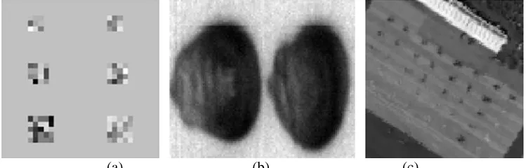
In our experiments, three HSI datasets are used as shown in Fig. 4. The first dataset in Fig. 4(a) is a simulated dataset with a size of 30×30 pixels, including 6 targets which lie in two columns. In each row, the two targets are of the same size varying from 3×3 to 4×4 and 5×5 pixels, thus all together we have 100 target pixels and 800 background pixels. Actually, the spectral data contained in this image are randomly selected form the third HSI dataset used in this paper as follows: Firstly, we arbitrarily select 100 target pixels from the original dataset, airport HSI dataset, based on the targets positioned in Fig. 4(c), and arrange them in rectangle windows as illustrated in Fig. 4(a). Secondly, 800 background pixels are also randomly chosen from the original dataset and arranged around the target pixels. Thus, the simulated dataset is constituted, where the number of spectral band, spectral and spatial resolution are all the same as them of the original dataset.
(a) (b) (c)
Fig. 4 Experimental dataset (band 60), (a) Imaging of simulated dataset, (b) Imaging of corn kernel dataset, (c) Imaging of airport dataset
The second HSI dataset, as shown in Fig. 4(b), is the corn kernel dataset, containing two corns in an image sized of 85×100 pixels. This dataset has 160 spectral bands and was obtained from Texas Agrilife Research (Texas A&M University). The HSI data were acquired with a line-scanning hyperspectral camera (PIKA II, www.resonon.com), which had 640 sensors producing HSI within a spatial resolution of 169 pixels/cm2 and a wavelength range from 405nm to 907 nm, i.e. a spectral resolution of 3.1 nm.
The angular field of view was set as 7 and the focal length of the objective lens was 35mm, optimized for the visible and near-infrared (NIR) spectra.
[image:9.612.119.495.391.511.2]10
absorption of water and low signal-to-noise, we use only 126 bands in our experiments. The image size is 100×100 pixels, containing 38 planes as targets for detection.
4.2 Experimental results and analysis
For performance evaluation, the experimental results are compared using both subjective and objective criteria. Visual inspection is employed for subjective evaluation of the detected target pixels, where the accuracy and robustness can be observed from the detected results. Quantitative comparison is utilized for objective evaluation, where the receiver operating characteristics (ROC) curves are used to present the probability of detection (PD) as a function of the probability of false alarms (PFA). The PFA is calculated by the number of false alarms (background pixels determined as target) over the total number of pixels in the test region, and the PD is the ratio of the number of hits (correctly detected target pixels) and the total number of true target pixels. To plot ROC curves, thousands of results in pairs of (PD, PFA) under various thresholds are generated, thus the ROC curves here are also able to validate the robustness of the algorithms towards any possible combination of thresholds. In addition, the running time of each approach is compared as an indicator of complexity.
For the three HSI datasets, one simulated one and two real ones, three approaches are applied for sparse representation based target detection, including the basic one without spatial support, namely BSR, and two improved ones. In order to facilitate analysis and discussion, we also denote sparse representation approaches using adaptive window and adaptive neighbourhood as AWSR and ANHSR, respectively. The percentage of pixels from the image to compose the dictionary is about 10%. And for the simulated and airport datasets, because of the spatial resolution, some pixels contained in them must be mixed pixels which contain the different kind information of the materials. Usually, the effect of mixing is highly dominant in HSI. However, in sparse representation, the atoms or pixels in dictionary are selected form the original image and they also contain the mixing information. Considering the same material of the airport background and the planes as targets, the mixing level would affect the results but it not very severe factor. So in this paper, the pixels are all considered as individuals to participate into experiments. Please note that for these three approaches the experimental settings are identical, i.e. the same target and background training atoms are used for all these three detectors.
For the first HSI dataset, the spectral signatures of the dictionary are collected directly from the top
left corner region of the simulated HSI data. The number of atoms in the dictionary is 100 with Nt=9 and Nb=91, i.e. 9 pixels from the targets and 91 pixels from the background in the region. The BP algorithm (Dai and Milenkovic 2009) is used to solve the sparse representation problem in Equation (6), while the sparse representation problem in Equation (16) is solved by using the simultaneous subspace pursuit (SSP) algorithm (Chen et al. 2011a).
11
[image:11.612.186.423.83.204.2](a) (b)
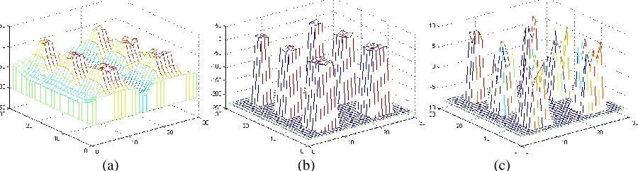
Fig. 5 Detection result (a) for the simulated HSI dataset, where (b) is the 60th band image.
To better illustrate the detection effect, the results are also plotted in 3-D and shown in Fig. 6, where more details can be observed than those from Fig. 5. As can be seen, the results from both ANHSR and AWSR have much higher and flat peaks. Higher peaks than those from BSR here mean the detected results are more robust as it allows a larger threshold to be applied to filter any potential false alarms. On the other hand, flat peaks mean that the results tend to be consistent to all target pixels, whilst results from BSR have much uneven peaks, which may lead to missing detection when a high threshold is applied as explained below.
(a) (b) (c)
Fig. 6 Experiment result for simulated HSI dataset in 3D version, (a) AWSR, (b) ANHSR, (c) BSR
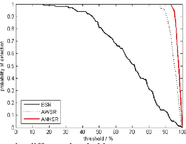
For the results from each of the three approaches above, the minimum and the maximum values of ( )
[image:11.612.90.540.334.455.2]12
Fig. 7 Probability of detection under different thresholds
For the second dataset, the spectral signatures of the dictionary are collected directly from pixels of the leftmost region in the given HSI. The number of atoms in the dictionary is 850, one over ten of all pixels, with Nt=292 and Nb=558, i.e. 292 target pixels and 558 background pixels are respectively
selected from the region. The detection results under the best prescribed threshold are shown in Fig. 8, and the 3-D version of the results are plotted in Fig. 9. In this group of experiments, AWSR and ANHSR produce very comparable results, and both of them outperform BSR in generating more accurate results with much less false alarms.
[image:12.612.100.510.353.470.2](a) (b) (c)
Fig. 8 Detection results for corn kernel dataset using AWSR (a), ANHSR (b) and BSR (c) methods.
[image:12.612.91.543.502.624.2](a) (b) (c)
Fig. 9 Experiment results for corn kernel dataset in 3-D version, (a) AWSR, (b) ANHSR, (c) BSR
13
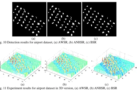
is 1000, one over ten of all pixels, with Nt=41 and Nb=959, i.e. 41 target pixels and 959 background pixels. The detection results for this dataset under the best prescribed threshold are given in Fig. 10, and the 3-D version of the detected results are also illustrated in Fig. 11. Again, we can easily find that AWSR and ANHSR yield much improved results than BSR, where more accurate results with much less false alarms are detected as shown in Fig. 10.
(a) (b) (c) Fig. 10 Detection results for airport dataset, (a) AWSR, (b) ANHSR, (c) BSR
[image:13.612.94.544.155.449.2](a) (b) (c) Fig. 11 Experiment results for airport dataset in 3D version, (a) AWSR, (b) ANHSR, (c) BSR
14
0 0.01 0.02 0.03 0.04 0.05 0.06 0.07 0.08 0.09 0.1
0.8 0.82 0.84 0.86 0.88 0.9 0.92 0.94 0.96 0.98 1
PFA
PD
AWSR ANHSR BSR
0 0.05 0.1 0.15 0.2 0.25 0.3 0.35 0.4 0.45 0.5
0.4 0.5 0.6 0.7 0.8 0.9 1
PFA
PD
AWSR
ANHSR BSR
[image:14.612.82.539.84.265.2](a) (b)
Fig. 12 ROC curves using AWSR, ANHSR and BSR approaches for the corn kernel dataset (a) and the airport dataset (b).
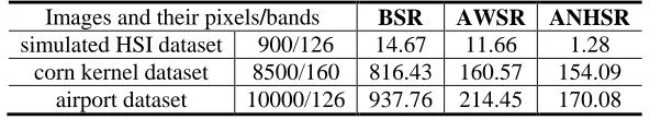
Finally, the running time of the three approaches on the three datasets are compared in Table 1 as an indicator of computational complexity. Although the absolute time used also depends on the pixels and bands of the dataset, for a given dataset the running time still provides a consistent measurement of complexity in this context. As can be seen, AWSR and ANHSR need much less time to achieve significantly improved results, whilst the reason behind is that the spatial support used has helped to smooth the inconsistency among spatial neighbouring pixels. As a result, the process of sparse representation can be easily recovered. In addition, it is found ANHSR is not only the most effective but also the most efficient approach for target detection from HSI datasets used in this study.
Table 1. Running time in seconds of the three approaches over the three datasets Images and their pixels/bands BSR AWSR ANHSR simulated HSI dataset 900/126 14.67 11.66 1.28
corn kernel dataset 8500/160 816.43 160.57 154.09 airport dataset 10000/126 937.76 214.45 170.08
5. Conclusion
In this paper, we propose two new sparse representation approaches based on adaptive window and neighbourhood for effective target detection in HSI. With the spatial support provided, both spatial correlation and spectral similarity of adjacent neighbouring pixels are used in constructing the optimized sparse representation. Using both visual inspection for subjective evaluation and ROC for quantitative evaluation, it is found the proposed approaches have significantly outperformed the conventional sparse representation method where spatial support is absent. In addition, sparse representation with adaptive neighbourhood support is found to be the best in dealing with complex cases, also the most efficient one with minimum running time required in recovering the sparse representation for fast and effective target detection.
Acknowledgements
[image:14.612.158.464.423.478.2]15
20102304110013). We also thank Dr. Kolomiets at Texas A&M University for providing codes of the corn kernels used in this study.
Reference
AHARON, M., ELAD, M., and BRUCKSTEIN, A., 2006, K-SVD: an algorithm for designing overcomplete dictionaries for sparse representation. IEEE Transactions on Signal Processing, 54, 4311-4322.
BANERJEE, A., BURLINA, P., and DIEHL, C., 2006, A support vector method for anomaly detection in hyperspectral imagery. IEEE Transactions on Geoscience and Remote Sensing, 44, 2282-2291.
BASRI, R., and JACOBS, D. W., 2003, Lambertian reflectance and linear subspaces. IEEE Transactions on Pattern Analysis and Machine Intelligence, 25, 218-233.
BIOUCAS-DIAS, J. M., and NASCIMENTO, J. M. P., 2008, Hyperspectral subspace identification. IEEE Transactions on Geoscience and Remote Sensing, 46, 2435-2445.
CHEN, S., and ZHANG, D., 2011, Semisupervised dimensionality reduction with pairwise constraints for hyperspectral image classification. IEEE Geoscience and Remote Sensing Letters, 8, 369-373.
CHEN, Y., NASRABADI, N. M., and TRAN, T. D., 2011a, Hyperspectral image classification using dictionary-based sparse representation. IEEE Transactions on Geoscience and Remote Sensing, 49, 3973-3985.
CHEN, Y., NASRABADI, N. M., and TRAN, T. D., 2011b, Sparse representation for target detection in hyperspectral imagery. IEEE Journal of Selected Topics in Signal Processing, 5, 629-640.
DAI, W., and MILENKOVIC, O., 2009, Subspace pursuit for compressive sensing signal reconstruction. IEEE Transactions on Information Theory, 55, 2230-2249.
EISMANN, M. T., STOCKER, A. D., and NASERBADI, N. M., 2009, Automated hyperspectral cueing for civilian search and rescue. Proceedings of the IEEE, 97, 1031-1055.
GU, Y., WANG, C., WANG, S., and ZHANG, Y., 2011, Kernel-based regularized-angle spectral matching for target detection in hyperspectral imagery. Pattern Recognition Letters, 2, 114-119.
HAQ, Q. S. U., TAO, L., SUN, F., and YANG, S., 2012, A fast and robust sparse approach for hyperspectral data classification using a few labeled samples. IEEE Transactions on Geoscience and Remote Sensing, 50, 2287-2302.
KRAUT, S., SCHARF, L. L., and MCWHORTER, L. T., 2001, Adaptive subspace detectors. IEEE Transactions on Signal Processing, 49, 1-16.
LI, S., and QI, H., 2011, Sparse representation based band selection for hyperspectral images. In 2011 18th IEEE International Conference on Image Processing, pp. 2693-2696.
MANOLAKIS, D., and SBAW, G., 2002, Detection Algorithm for Hyperspectral Imaging Applications. IEEE Signal Processing Magazine, 19, 29-43.
MELGANI, F., and BRUZZONE, L., 2004, Classification of hyperspectral remote sensing images with support vector machines. IEEE Transactions on Geoscience and Remote Sensing, 42, 1778-1790.
MURPHY, R. J., MONTEIRO, S. T., and SCHNEIDER, S., 2012, Evaluating classification techniques for mapping vertical geology using field-based hyperspectral sensors. IEEE Transactions on Geoscience and Remote Sensing, 50, 3066-3080.
NGUYEN, D. T., CHEN, Y., TRAN, T. D., and CHIN, S. P., 2011, Simultaneous sparse recovery for unsupervised hyperspectral unmixing. In Proceedings of SPIE - The International Society for Optical Engineering.
REED, I. S., and YU, X., 1990, Adaptive Multi-Band CFAR Detection of an Optical Pattern with Unknown Spectral Distribution. IEEE Transactions on Acoustics Speech and Signal Processing, 38, 1760-1770. RUBINSTEIN, R., BRUCKSTEIN, A. M., and ELAD, M., 2010, Dictionaries for sparse representation
modeling. Proceedings of the IEEE, 98, 1045-1057.
SCHARF, L. L., and FRIEDLANDER, B., 1994, Matched subspace detectors. IEEE Transactions on Signal Processing, 42, 2146-2157.
16
TITS, L., SORNERS, B., and COPPIN, P., 2012, The potential and limitations of a clustering approach for the improved efficiency of multiple endmember spectral mixture analysis in plant production system monitoring. IEEE Transactions on Geoscience and Remote Sensing, 50, 2273-2286.
TROPP, J. A., and GILBERT, A. C., 2007, Signal recovery from random measurements via orthogonal matching pursuit. IEEE Transactions on Information Theory, 53, 4655-4666.
WRIGHT, J., MA, Y., MAIRAL, J., SAPIRO, G., HUANG, T. S., and YAN, S., 2010, Sparse representation for computer vision and pattern recognition. Proceedings of the IEEE, 98, 1031-1044.