Fatigue Damage Evaluation Using Electron Backscatter Diffraction

Fatigue Damage Evaluation Using Electron Backscatter Diffraction

Masayuki Kamaya

and Masatoshi Kuroda

1

Institute of Nuclear Safety System, Inc., 64 Sata, Mihama-cho, Mikata-gun, Fukui 919-1205, Japan

2_{Department of Mechanical System Engineering, Graduate School of Science and Technology, Kumamoto University,} 2-39-1, Kurokami, Kumamoto 860-8555, Japan

It is important to identify residual strength against fatigue damage to ensure the structural integrity of plant components subjected to cyclic loading. In this study, the degree of fatigue damage induced in Type 316 stainless steel was estimated from the local change in crystal orientation (local misorientation) measured by electron backscatter diffraction (EBSD). Crystal orientations were identified by scanning the surfaces of samples that had been subjected to a fatigue test or a tensile test. The magnitude of the averaged local misorientation,Mave, increased as the strain

amplitude and the number of cycles increased, and the relationship between strain amplitude, number of cycles andMavewas obtained.

Moreover, from the correlation betweenMaveand another parameter,MCD, which reflects the average of the orientation spread within the

grains, it was shown to be possible to distinguish whether damage was caused by cyclic loading or monotonic loading. Further investigation of the local misorientation revealed that the amplitude of fatigue loading could be estimated from the statistical distribution of local misorientation averaged for each grain. It was concluded that fatigue damage (residual fatigue strength) could be quantified by EBSD measurements using the estimated strain amplitude and the relationship between strain amplitude, number of cycles andMave. [doi:10.2320/matertrans.M2011014]

(Received January 11, 2011; Accepted March 11, 2011; Published May 18, 2011)

Keywords: electron backscatter diffraction (EBSD), low-cycle fatigue, stainless steel, local misorientation, fatigue damage

1. Introduction

In the structural design of nuclear power plant compo-nents, the damage due to cyclic loading (fatigue damage) is taken into account by ensuring that the cumulative fatigue damage during plant operation does not exceed the fatigue strength of the material.1) _{The fatigue damage is evaluated} using the amplitude of cyclic loading and the number of cycles estimated during plant operation. The main source of cyclic loading is the thermal stress arising during transition of operating conditions such as start-up and shut-down of the plant. However, due to the difficulty of evaluating the thermal stress, uncertain factors are considered conservatively in the design for the sake of simplicity.2)_{Moreover, a high safety} margin is set for the fatigue strength of the material used in the design.3) Accordingly, damaged components can often continue to be used without taking countermeasures even if the evaluated fatigue damage exceeds the design criterion.4) Therefore, it is important to measure the true fatigue damage induced in the material.

In order to measure the fatigue damage, it is necessary to clarify the process by which the material is damaged. There are two main kinds of fatigue damage: surface cracking and bulk damage. Murakami and Miller5)_{showed, through} low-cycle fatigue tests of S45C, that the fatigue life was dominated by surface crack growth and that the Manson-Coffin relation could be regarded as an alternative expression for the crack growth law, which is determined by the crack length and applied stress/strain. This concept was confirmed by experimental results, in which fatigue life was extended when the surface layer of specimens was removed during the fatigue test.6,7)On the other hand, it was pointed out that not only surface cracking but also additional damage (hereafter called ‘‘bulk damage’’) accumulates in the material due to cyclic loading and reduces the fatigue life.8–12)In a previous study by one of the authors,13)_{it was shown that the local} change in crystal orientation (local misorientation), which

was caused by the bulk damage, was closely correlated with crack initiation in a low-cycle fatigue test of Type 316 stainless steel.

Once a crack is initiated in a component, the degree of fatigue damage and the residual strength can be evaluated based on the size of the crack.14–16)_{However, the resolution} and accuracy of crack detection are insufficient for evaluating the fatigue damage at an early stage, which dominates the fatigue life of components. On the other hand, the bulk damage accumulates continuously from the start of plant operation. The degree of bulk damage can be evaluated by observing the evolution of defects using transmission electron microscopy17)_{or by measuring the density of defects} using positron annihilation18)_{or ultrasonic attenuation.}19)_In particular, electron backscatter diffraction (EBSD) is one of the most promising techniques for assessing crystal lattice defects over a large range from several tens of nanometers to several millimeters.20,21) Cyclic plastic strain leads to the occurrence of geometrically necessary dislocations by crys-tallographic slip, and local misorientation develops as a results. EBSD in conjunction with scanning electron mi-croscopy (SEM) can quantify the degree of local misorienta-tion from measured crystal orientamisorienta-tions.

In this study, EBSD was used to quantitatively evaluate the fatigue damage induced in Type 316 stainless steel, which is commonly used in nuclear power plant compo-nents. Firstly, low-cycle fatigue tests were conducted and fatigue damage was induced in the material. Then, the change in crystal orientations was measured using EBSD. Finally, by characterizing the microstructural change of the damaged sample, the magnitude of fatigue damage was correlated with parameters derived from measured crystal orientations.

2. Experimental Procedure

treated Type 316 austenitic stainless steel; its alloying constituents and mechanical properties are given in Tables 1 and 2, respectively. The material had an approximately equiaxed grain structure with an average grain diameter of 50mm. Round bar specimens (gauge length = 20 mm and diameter = 10 mm) were subjected to fully reversed axial strain-controlled fatigue tests, which were conducted in ambient air at room temperature under constant nominal strain amplitude"aof 0.5%, 0.6%, 0.7%, 1.0% and 1.5%. The rate of strain during the test was kept constant at 0.4%/s. Under "a of 0.5%, 1.0% and 1.5%, additional fatigue tests were performed, in which tests were stopped at 10%, 50% and 80% of fatigue life, which was defined by eq. (1) in the following section.

For comparison, tensile tests were also performed using the same material and the same geometry of the specimen. The tests were stopped at different magnitudes of plastic strain "p of 2.0%, 4.4% and 9.7% in nominal strain. The displacement rate was 1.0 mm/min at the cross-head of the tensile test machine.

After the tests, the specimens were then subjected to EBSD measurements; the cross section at an unbroken portion was observed. The surface of the sample was polished with diamond paste up to 3mm followed by colloidal silica polishing in order to achieve a relatively flat surface free from damage. Crystal orientations were measured by a commercial EBSD data acquisition system (OIM Data Collection ver. 5.2) interfaced to a field emission electron gun SEM (Carl Zeiss ULTRA55) operating at 20 keV. The crystal orientation maps were obtained by scanning over the range of250250mmwith the step size of 0.5mm. In order to perform accurate measurements, the number of pixels of the CCD camera used for EBSD pattern acquisition was set to the maximum (640480) and parameters for data processing of obtained diffraction patterns were selected carefully. Five maps were obtained for each sample including the untested (undamaged) sample. The obtained crystal orientations were processed by in-house developed software.22)

The names of the samples for EBSD measurement follow the convention: type of loading (F: Fatigue, T: Tensile), amplitude of the strain and ratio of number of cycles to fatigue life. For example, the sample from the fatigue test with strain amplitude of 1.5% subjected to the number of cycles that was 80% of the fatigue life is denoted as ‘‘F-1.5%80Nf’’, and that from the tensile test of plastic strain of 4.0% is denoted as ‘‘T-4.0%’’.

3. Results and Discussion

3.1 Fatigue tests

The obtained fatigue life curve is shown in Fig. 1 and the test results are summarized in Table 3. The number of cycles to failure, Nf(exp), was defined as the number when the maximum stress during the cycle dropped below 75% of the peak stress at half of the number of cycles. The regression curve is represented by:

"a¼14:1N_f 0:422 ð1Þ

where Nf and "a denote the fatigue life and the strain amplitude in percent, respectively. The change in the variation of the peak stress during the fatigue tests is shown in Fig. 2. A rapid cyclic hardening occurred at the beginning of each test, followed by a continuous increase in the stress. The degree of hardening increased with the applied strain, whereas the stress remained nearly constant at less than "a¼0:7%.

Table 1 Chemical content of test material (mass%).

Fe C Si Mn P S Ni Cr Mo

Bal. 0.05 0.26 1.29 0.035 0.028 10.00 16.81 2.00

Table 2 Mechanical properties of test material.

0.2% proof strength

Tensile

strength Elongation

Reduction of area

278 MPa 602 MPa 0.58 0.74

0.1 1.0 10.0

100 1000 10000

Strain amplitude,

a

(%)

ε

Number of cycles at failure, Nf

Fig. 1 Fatigue life of test material.

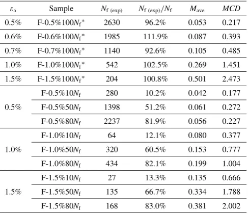
Table 3 Summarized results of fatigue tests.

"a Sample Nf (exp) Nf (exp)=Nf Mave MCD

0.5% F-0.5%100Nf 2630 96.2% 0.053 0.217

0.6% F-0.6%100Nf 1985 111.9% 0.087 0.393

0.7% F-0.7%100Nf 1140 92.6% 0.105 0.485

1.0% F-1.0%100Nf 542 102.5% 0.269 1.451

1.5% F-1.5%100Nf 204 100.8% 0.501 2.473

F-0.5%10Nf 280 10.2% 0.042 0.177

0.5% F-0.5%50Nf 1398 51.2% 0.061 0.272

F-0.5%80Nf 2237 81.9% 0.056 0.227

F-1.0%10Nf 64 12.1% 0.080 0.377

1.0% F-1.0%50Nf 320 60.5% 0.153 0.777

F-1.0%80Nf 434 82.1% 0.199 1.004

F-1.5%10Nf 27 13.3% 0.135 0.666

1.5% F-1.5%50Nf 135 66.7% 0.334 1.788

F-1.5%80Nf 168 83.0% 0.381 2.002

3.2 Local misorientation map

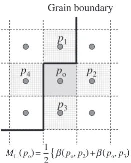
Based on the crystal orientations obtained by the EBSD measurement, the local misorientation, ML, was calculated by the following equation:23)

MLðpoÞ ¼ 1

4

X4

i¼1

ðpo;piÞ ð2Þ

whereðpo;piÞdenotes the misorientation between a fixed point po and neighboring points pi in the same grain as depicted in Fig. 3. A line was drawn between two adjacent points when the misorientation was larger than 5_{. If a series} of the lines formed a closed region, the lines were defined as a

grain boundary, and the misorientation between the points of different grains was not included in the calculation ofML.

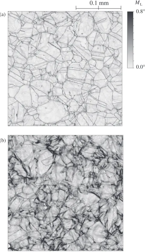
Mapping data of the local misorientations for one sample obtained under"a¼1:0% are shown in Fig. 4. Although the EBSD measurement was performed carefully in order to obtain accurate crystal orientations, the distribution of local misorientations was not clear. The local misorientations in Fig. 4(a) were mostly less than 0.5_{, which was smaller than} the typical 0.5–1 _{error in crystal orientation measurements} by EBSD.24) _{Therefore, it was deduced that the local} misorientation map contained significant errors. In order to reduce the error in local misorientations and to obtain a clear and smooth map, the following filtering process was adopted.25) To remove the error in the crystal orientations obtained, the average of the crystal orientations of surround-ing points (up to nine points) was calculated for each point as schematically shown in Fig. 5. Then, the local misorienta-tions were calculated using the filtered crystal orientamisorienta-tions. Since this filtering process includes the repetition of averag-ing of measured crystal orientation,26,27) _{the resultant local} -800

-600 -400 -200 0 200 400 600 800

1 10 100 1000 10000

Peak stress,

/MP

a

σ

Number of cycles N

F-1.5% F-1.0% F-0.7% F-0.6% F-0.5%

Fig. 2 Change in peak stress during fatigue tests.

p

p

p

p

p

L

1 4

M β β β β

p

p

p

p

p

Grain boundary

L

1 2 M

(po)=

{

β β

(po)=

{

Fig. 3 Definition of local misorientation.

ML

0.8°

0.0°

(a)

0.1 mm

(b)

Fig. 4 Local misorientation maps for one sample after the fatigue test (F-1.0%100Nf). (a) Without filtering process (b) After filtering process

misorientation may blur the characteristics of the distribu-tion. However, unmeaning error can be reduced significantly. Figure 4(b) shows the local misorientation map after apply-ing the filterapply-ing process. The error in the local misorientations was successfully reduced and the map became clearer. This filtering process was applied to all data in the following analyses.

Figure 6 shows the local misorientation maps for two samples of different strain amplitude. The magnitude of the local misorientation increased with strain amplitude. In particular, in the case of"a¼1:5%, the local misorientation increased significantly. In these maps, grains consisting of less than 10 points are indicated by white pixels. If the crystal orientation was not identified correctly in the measurement, such a point constituted an isolated small grain and it was indicated by a white pixel. Some clusters of white pixels were observed in the maps of large strain amplitude. The diffraction pattern suggested that most of the white pixels corresponded to bcc crystal structure (martensite structure). The positions of the martensite structure correlated well with large local misorientations. In all cases, the development of local misorientation was not homogeneous but it was localized. Even in the case of "a¼0:5%, the local misor-ientation became large locally (hereafter called a ‘‘localized region’’). The spacing between localized regions ranged from 50 to 100mm.

Figure 7 shows the maps for "a¼1:0% for different numbers of cycles. The local misorientation increased as the number of cycles increased. In the map of F-0.5%10Nf, some localized regions could be found, and such regions were considered to be nuclei for localization of the local misorientation in the following cycles. In the low-cycle fatigue test in the previous paper, microstructurally small cracks were preferentially initiated at the localized regions,13) suggesting that the local misorientation was a kind of bulk damage. Therefore, by evaluating the change in the magni-tude of the local misorientation, the degree of fatigue damage can be estimated.

Local misorientation also developed due to plastic strain under monotonic loading as shown in Fig. 8. However, the characteristic of the distribution of local misorientation was slightly different from that of the fatigue samples. In the tensile samples, the degree of localization was relatively low

and spread over the whole area, and the local misorientation tended to be large near grain boundaries or their junction points. As pointed out in the previous study,28)in tensile tests, the local misorientation easily develops near grain bounda-ries due to the pile-up of dislocations. No localization was found in the sample of T-2.2%.

3.3 ParametersMaveandMCD

For a quantitative evaluation two parameters were calcu-lated from obtained crystal orientations: the averaged local misorientationMave23)and the modified crystal deformation

MCD.29)_M

avewas calculated as the log-normal mean of the local misorientation by the following equation:

Mave¼exp 1

n

Xn

i¼1

lnfMLðpiÞg

" #

ð3Þ

where n is the number of data. It was shown that Mave correlated well with the degree of plastic strain induced by tensile tests.23)_{On the other hand,MCDwas defined by the} following equation:29)

Grain boundary

Position for EBSD measurement

Measured crystal orientation was replaced with average of 9 orientations

At the corner, 4 orientations were averaged.

Fig. 5 A schematic drawing of the smoothing filter for crystal orientations.

0.1 mm

(a)

(b)

M_L

0.8°

0.0°

Fig. 6 Local misorientation maps for two samples after fatigue tests under different strain amplitudes. (a) F-0.5%100Nf (Mave¼0:053)

MCD¼exp

Xng

k¼1 Xnk

i¼1

lnfðmk;piÞg

( )

Xng

k¼1 nk

2 6 6 6 6 4

3 7 7 7 7

5: ð4Þ

Again, ðmk;piÞ denotes the misorientation between the central orientation, m, of the kth grain and the point i that belongs to the kth grain, and nk is the number of points included in the grain.ngis the number of grains. The central orientation was determined as the averaged crystal orienta-tion of all points included in the grain (see Fig. 9). The parameterMCDwas also shown to be linearly correlated with plastic strain up to 15%.29)These parameters were calculated for each map and the mean value of the five maps was as summarized in Table 3.

The change inMaveof fatigue and tensile samples is shown in Fig. 10, in which the mean value and variations in five maps are indicated. Mave was 0.037 for the undamaged sample and increased with strain amplitude and number of

cycles, although it was almost the same under "a¼0:5%. Therefore, it is possible to estimate the degree of fatigue damage by evaluatingMave. However, in order to determine the residual fatigue strength of the damaged material based on the fatigue life curve, it is necessary to identify two independent parameters: the strain amplitude and the number of cycles. Therefore, to estimate the fatigue damage from Fig. 10(a), the strain amplitude or the number of cycles must be specified.

Mavewas also dependent on the plastic strain as shown in Fig. 10(b). The variation in the five maps seemed to be less than that of the fatigue samples. This suggests that the scanning range of250250mmis large enough to disregard the microstructural inhomogeneity formed by the tensile test. The change in MCD exhibited a similar tendency with the number of cycles and plastic strain.

Figure 11 shows the relationship between the averaged local misorientation Mave and the parameter MCD. The results from five maps for each specimen are plotted in Fig. 11.MaveandMCDwere closely correlated and increased

0.1 mm

(a)

(b)

ML

0.8°

0.0°

Fig. 7 Local misorientation maps for two samples of different fatigue damages. (a) F-1.0%10Nf (Mave¼0:083) (b) F-1.0%80Nf (Mave¼

0:184_).

0.1 mm

(a)

(b)

ML

0.8°

0.0°

as the strain amplitude increased. The inclination of the regression line was different for the fatigue and tensile samples. Accordingly, it is possible to discern whether the source of damage is cyclic loading or monotonic loading by evaluating the correlation betweenMaveandMCD.

3.4 Rotation axis of misorientation

In order to identify the reason for the difference in the correlation of Mave and MCD between the fatigue and tensile samples, misorientation axis was examined. When the misorientation angles are calculated from two crystal orientations, the rotation axis of misorientation is identified as well. The change in the rotation axis was visualized by assigning colors so that the contrast was maximized.30) Figure 12 shows the rotation axis of the misorientation from the central orientation, which is the averaged crystal orientation evaluated for each grain (Fig. 9). The color notation was determined so that the maximum value of the horizontal component of the vector was assigned the maximum intensity of red, while the minimum value was assigned to the minimum intensity of red, and similarly the vertical and normal components were assigned maximum and minimum intensities of green and blue. The vector of rotation axis was then transferred into red-green-blue (RGB) space. It should be stressed that each grain is given a different color code and that comparisons between color and intensity of different data points are only valid when they belong to the same grain. This visualization allows examination of how the crystal orientation fluctuated inside the grain. The fatigue sample showed a frequent change of the rotation axis, whereas that of the tensile sample changed monotonically. In the tensile samples, due to relatively large strain, the whole of the specimen was deformed and exhibited a monotonous change of the rotation axis inside the grain. On the contrary, in the fatigue samples, the magnitude of the strain was not enough to develop the local misorientation spread over the sample as shown in Fig. 7(a), which indicated only a few localized regions. The fluctua-tion of the rotafluctua-tion axis was attributed to the repetifluctua-tion of small strain.

Inverse pole figure

Grain boundary

(111)

(101) (100)

Central orientation of grain k (m_k)

Misorientation between central orientation and point i

(m_k , p_i )

β

Fig. 9 A schematic drawing representing the concept of parameter MCD.

0.0°

0.1°

0.2°

0.3°

0 2 4 6 8 10

Mave

Plastic strain, ε_p(%)

0.0°

0.1°

0.2°

0.3°

0.4°

0.5°

0.6°

0.0 0.2 0.4 0.6 0.8 1.0

M

ave

N/Nf 0.0

0.5 1.0 1.5 0.6 0.7 a(%)

ε

(a)

(b)

Fig. 10 Averaged local misorientations. (a) Fatigue sample (b) Tensile sample.

0.0° 0.1° 0.2° 0.3° 0.4° 0.5° 0.6°

0° 1° 2° 3°

Mave

MCD Undamged

F-0.5% F-0.6% F-0.7% F-1.0% F-1.5% T-2.2% T-4.0% T-9.7%

Figure 13 schematically shows the change in crystal orientation in the fatigue and tensile samples. The fatigue sample exhibited relatively large fluctuation in the crystal orientation. Since the parameter Mave is the average of the misorientation between neighboring points, the fluctuation in the crystal orientation madeMavelarger. On the other hand,

MCD was not influenced by the local change in the crystal orientation because it is the misorientation from the central orientation. Namely, in Fig. 13,Mavecorresponds to differ-entiation of the crystal orientation curve, while MCD corresponds to integration of the curve. Therefore, MCD reflects the deformation of the whole grain and does not take

into account the local change in the crystal orientation at each point. It is worth mentioning that the magnitude ofMCDdoes not depend on the step size in the EBSD measurement.29) Accordingly, even ifMCDwas the same,Maveof the fatigue samples tended to be larger than that of the tensile samples.

3.5 Grain-averaged local misorientation

The change in crystal orientation grain by grain was investigated next; the change within grains was discussed in Fig. 12. Figure 14 shows the local misorientation averaged for each grain (hereafter called ‘‘grain-averaged local misorientation (Mave(g))’’) for samples F-1.0%100Nf and T-9.7%, whose local misorientation maps are shown in Figs. 4(b) and 8(b), respectively. The variation inMave(g)was larger for the fatigue sample, althoughMaveof these figures was almost the same: 0.286 and 0.260 for the fatigue and tensile samples, respectively. In the tensile samples, due to relatively large strain, the local misorientation developed throughout the whole map and the scatter in Mave(g) was suppressed. On the other hand, in the fatigue sample, the 0.1 mm

(a)

(b)

Fig. 12 Rotation axis of misorientation from the central orientation for each grain. (a) F-1.0%100Nf(b) T-9.7%.

Position

Crystal orientation

Crystal orientation

Tensile sample Fatigue sample

M_ave

Mave

MCD

MCD

Fig. 13 A schematic drawing of the change in crystal orientation due to fatigue and tensile tests and its effect on the parametersMaveandMCD.

0.1 mm

(a)

(b)

M_L

0.8°

0.0°

Fig. 14 Grain-averaged local misorientation (Mave(g)) for fatigue and

tensile samples. (a) F-1.0%100Nf(Mave¼0:286) (b) T-9.7% (Mave¼

deformation was localized andMave(g) was larger for certain grains. The magnitude of Mave(g) seemed to depend on the grain size; smaller grains showed larger local misorientation. This tendency was also observed in the samples of small strain amplitude as shown in Figs. 6(a) and 7(a), whereas the tensile sample with a similar value of Mave showed no localized region as shown in Fig. 8(a). Hence, the degree of localization depended on the strain amplitude and it can be evaluated by the variations inMave(g).

Mave(g)was then calculated for each map. Figure 15 shows

the frequency distribution obtained from five maps of the F-1.0%80Nf sample. The number of data (grains) was typically more than 2000 from five maps, and the distribution was regarded as log-normal. Figure 16 shows the relationship between the log-normal mean and the log-normal standard deviation of Mave(g). The standard deviation was relatively small for the tensile samples and the fatigue samples of large strain amplitude, and it increased as the number of cycles increased except for samples F-1.0%100Nf and F-1.5%100Nf. In particular, in the case of "a¼0:5%, the standard deviation increased monotonically, although Mave remained almost constant as shown in Fig. 10(a). Since the inclination of the correlation curve in Fig. 16 depended on the strain amplitude, it was possible to estimate the strain amplitude of the fatigue loading. Namely, large strain amplitude caused a relatively uniform distribution of local misorientation and relatively small standard deviation of

Mave(g). On the other hand, small strain amplitude resulted in

inhomogeneous development of the local misorientation and caused a relatively large standard deviation of Mave(g). The standard deviation of the local misorientation also exhibited a similar dependency on the strain amplitude, although the dependency was not as clear as that ofMave(g).

As mentioned earlier, in order to measure the residual fatigue strength of a damaged material based on the fatigue life curve, it is necessary to identify the strain amplitude and the number of cycles. Since the strain amplitude can be identified using the correlation of Fig. 16, it is possible to estimate the number of cycles toNf(residual fatigue strength) by evaluatingMavebased on the relation shown in Fig. 10(a).

4. Conclusions

In order to quantify the degree of fatigue damage of Type 316 stainless steel, EBSD observations were made for samples subjected to fatigue or tensile tests. Based on the crystal orientations obtained by scanning the sample surface, mapping data of the local misorientation were obtained. The local misorientation increased as the strain amplitude and the number of cycles increased, and the relationship between the number of cycles and the averaged local misorientationMave was quantified. Moreover, from the correlation betweenMave and another parameter, MCD, obtained from the crystal orientations, it was demonstrated to be possible to distinguish whether damage was caused by cyclic loading or monotonic loading. Further investigation of the local misorientation revealed that the amplitude of fatigue loading correlated well with the statistical distribution of Mave(g), and that it was possible to estimate the strain amplitude. It was concluded that the fatigue damage (residual fatigue strength) could be quantified by EBSD measurements using the estimated strain amplitude and the relationship between strain amplitude, number of cycles andMave.

Acknowledgements

The authors express special thanks to Mr. Y. Imamura, Mr. T. Yasuda and Mr. T. Daiba for their help with the fatigue tests.

REFERENCES

1) ASME boiler and pressure vessel code section III, (ASME, New York, 2007).

2) T. Nakamura, M. Iwasaki and S. Asada: Proc. ASME 2007 Pressure Vessels and Piping Conference, (American Society of Mechanical Engineers, 2007) no. 26247.

3) C. E. Jaske and W. J. O’Donnell: ASME J. Pressure Vessel Technology 99(1977) 584–592.

4) ASME boiler and pressure vessel code section XI appendix L, (ASME, New York, 2007).

5) Y. Murakami and K. J. Miller: Int. J. Fatigue27(2005) 991–1005. 6) M. Kikukawa, K. Ohji, H. Ohkubo, T. Yokoi and T. Morikawa: Trans. 0.00 0.02 0.04 0.06 0.08 0.10 0.12 0.14 0.16 0.18 0.20 0.1 ° 0.2 ° 0.4 ° 0.5 ° 0.7 ° 0.8 ° 1.0 ° 1.1 ° 1.3 ° Frequency

Grain averaged local misorientation

Measurement data

Log-normal distribution

Number of data: 2281

Fig. 15 Frequency distribution of grain-averaged local misorientation (F-1.0%80Nf).

1.2° 1.3° 1.4° 1.5° 1.6° 1.7° 1.8° 1.9°

0.0° 0.2° 0.4° 0.6° 0.8°

Standard de

viation of

Mav

e(g)

Mean of Mave(g) F-1.5% F-1.0% F-0.6% F-0.7% F-0.5% Tensile sample undamaged sample

Japan Soc. Mech. Eng.38(1972) 8–15.

7) H. Nishitani and T. Morita: Trans. Japan Soc. Mech. Eng.39(1973) 1711–1719.

8) N. Ohtani, T. Abe, M. Shimizu and T. Kunio: Trans. Japan Soc. Mech. Eng. A45(1979) 1304–1311.

9) K. Shimada, J. Komotori and M. Shimizu: Trans. Japan Soc. Mech. Eng. A53(1987) 1178–1185.

10) J. Komotori and M. Shimiizu: Trans. Japan Soc. Mech. Eng. A57 (1991) 2879–2883.

11) M. Kuroda: Int. J. Fatigue24(2001) 699–703.

12) K. Tateishi, T. Hanji and K. Minami: Int. J. Fatigue29(2007) 887–896. 13) M. Kamaya: Fatigue Fracture Eng. Mater. Struct.33(2009) 94–104. 14) JSME Fitness-For-Service Code S NA1-2004, (JSME, Tokyo, 2004). 15) Guide to methods for assessing the acceptability of flaws in metallic

structures BS 7910, (British Standards Institution, London, 2005). 16) Fitness-For-Service API 579, (American Petroleum Institute,

Washington, D.C., 2000).

17) T. Petersmeier, U. Martint, D. Eifler and H. Oettelt: Int. J. Fatigue20 (1998) 251–255.

18) N. Maeda, N. Nakamura, M. Uchida, Y. Ohta and K. Yoshida: Nuclear

Eng. Design167(1996) 169–174.

19) T. Ohtani, K. Nishiyama, S. Yoshikawa, H. Ogi and M. Hirao: Mater. Sci. Eng. A442(2006) 466–470.

20) L. N. Brewer, M. A. Othon, L. M. Young and T. M. Angeliu: Microsc. Microanal.12(2006) 85–91.

21) E. Demir, D. Raabe, N. Zaafarani and S. Zaefferer: Acta Mater.57 (2009) 559–569.

22) M. Kamaya, A. J. Wilkinson and J. M. Titchmarsh: Nuclear Eng. Design235(2005) 713–725.

23) M. Kamaya: Mater. Charact.60(2009) 125–132. 24) A. J. Wilkinson: Scr. Mater.44(2001) 2379–2385. 25) M. Kamaya: Mater. Trans.51(2010) 1516–1520. 26) F. J. Humphreys: J. Mater. Sci.36(2001) 3833–3854. 27) F. J. Humphreys: Scr. Mater.51(2004) 771–776. 28) M. Kamaya: Mater. Charact.60(2009) 1454–1462.

29) M. Kamaya, A. J. Wilkinson and J. M. Titchmarsh: Acta Mater.54 (2006) 539–548.