Using Supervised Bigram-based ILP for Extractive Summarization
Chen Li, Xian Qian, and Yang Liu
The University of Texas at Dallas Computer Science Department
chenli,qx,[email protected]
Abstract
In this paper, we propose a bigram based supervised method for extractive docu-ment summarization in the integer linear programming (ILP) framework. For each bigram, a regression model is used to es-timate its frequency in the reference sum-mary. The regression model uses a vari-ety of indicative features and is trained dis-criminatively to minimize the distance be-tween the estimated and the ground truth bigram frequency in the reference sum-mary. During testing, the sentence selec-tion problem is formulated as an ILP prob-lem to maximize the bigram gains. We demonstrate that our system consistently outperforms the previous ILP method on different TAC data sets, and performs competitively compared to the best results in the TAC evaluations. We also con-ducted various analysis to show the im-pact of bigram selection, weight estima-tion, and ILP setup.
1 Introduction
Extractive summarization is a sentence selection problem: identifying important summary sen-tences from one or multiple documents. Many methods have been developed for this problem, in-cluding supervised approaches that use classifiers to predict summary sentences, graph based ap-proaches to rank the sentences, and recent global optimization methods such as integer linear pro-gramming (ILP) and submodular methods. These global optimization methods have been shown to be quite powerful for extractive summarization, because they try to select important sentences and remove redundancy at the same time under the length constraint.
Gillick and Favre (Gillick and Favre, 2009) in-troduced the concept-based ILP for
summariza-tion. Their system achieved the best result in the TAC 09 summarization task based on the ROUGE evaluation metric. In this approach the goal is to maximize the sum of the weights of the lan-guage concepts that appear in the summary. They used bigrams as such language concepts. The as-sociation between the language concepts and sen-tences serves as the constraints. This ILP method is formally represented as below (see (Gillick and Favre, 2009) for more details):
max Piwici (1)
s.t. sjOccij ≤ci (2)
P
jsjOccij ≥ci (3)
P
jljsj ≤L (4)
ci∈ {0,1} ∀i (5)
sj ∈ {0,1} ∀j (6)
ci and sj are binary variables (shown in (5) and (6)) that indicate the presence of a concept and a sentence respectively. wi is a concept’s weight and Occij means the occurrence of concept i in sentence j. Inequalities (2)(3) associate the sen-tences and concepts. They ensure that selecting a sentence leads to the selection of all the concepts it contains, and selecting a concept only happens when it is present in at least one of the selected sentences.
There are two important components in this concept-based ILP: one is how to select the con-cepts (ci); the second is how to set up their weights (wi). Gillick and Favre (Gillick and Favre, 2009) used bigrams as concepts, which are selected from a subset of the sentences, and their document fre-quency as the weight in the objective function.
In this paper, we propose to find a candidate summary such that the language concepts (e.g., bi-grams) in this candidate summary and the refer-ence summary can have the same frequency. We expect this restriction is more consistent with the
ROUGE evaluation metric used for summarization (Lin, 2004). In addition, in the previous concept-based ILP method, the constraints are with respect to the appearance of language concepts, hence it cannot distinguish the importance of different lan-guage concepts in the reference summary. Our method can decide not only which language con-cepts to use in ILP, but also the frequency of these language concepts in the candidate summary. To estimate the bigram frequency in the summary, we propose to use a supervised regression model that is discriminatively trained using a variety of features. Our experiments on several TAC sum-marization data sets demonstrate this proposed method outperforms the previous ILP system and often the best performing TAC system.
2 Proposed Method
2.1 Bigram Gain Maximization by ILP
We choose bigrams as the language concepts in our proposed method since they have been suc-cessfully used in previous work. In addition, we expect that the bigram oriented ILP is consistent with the ROUGE-2 measure widely used for sum-marization evaluation.
We start the description of our approach for the scenario where a human abstractive summary is provided, and the task is to select sentences to form an extractive summary. Then Our goal is to make the bigram frequency in this system sum-mary as close as possible to that in the reference. For each bigramb, we define its gain:
Gain(b, sum) = min{nb,ref, nb,sum} (7) wherenb,ref is the frequency ofbin the reference summary, andnb,sumis the frequency of bin the automatic summary. The gain of a bigram is no more than its frequency in the reference summary, hence adding redundant bigrams will not increase the gain.
The total gain of an extractive summary is de-fined as the sum of every bigram gain in the sum-mary:
Gain(sum) =X
b
Gain(b, sum)
=X
b
min{nb,ref,
X
s
z(s)∗nb,s} (8)
where s is a sentence in the document, nb,s is the frequency of bin sentences,z(s)is a binary variable, indicating whether s is selected in the
summary. The goal is to find z that maximizes Gain(sum) (formula (8)) under the length con-straintL.
This problem can be casted as an ILP problem. First, using the fact that
min{a, x}= 0.5(−|x−a|+x+a), x, a≥0
we have
X
b
min{nb,ref,
X
s
z(s)∗nb,s}=
X
b
0.5∗(−|nb,ref −
X
s
z(s)∗nb,s|+
nb,ref+
X
s
z(s)∗nb,s)
Now the problem is equivalent to:
max
z
X
b
(−|nb,ref −
X
s
z(s)∗nb,s|+
nb,ref +
X
s
z(s)∗nb,s)
s.t. X
s
z(s)∗ |S| ≤L; z(s)∈ {0,1}
This is equivalent to the ILP:
max X
b
(X
s
z(s)∗nb,s−Cb) (9)
s.t. X
s
z(s)∗ |S| ≤L (10)
z(s)∈ {0,1} (11)
−Cb ≤nb,ref−
X
s
z(s)∗nb,s≤Cb
(12) whereCbis an auxiliary variable we introduce that is equal to|nb,ref−Psz(s)∗nb,s|, andnb,ref is a constant that can be dropped from the objective function.
2.2 Regression Model for Bigram Frequency Estimation
In the previous section, we assume that nb,ref is at hand (reference abstractive summary is given) and propose a bigram-based optimization frame-work for extractive summarization. However, for the summarization task, the bigram frequency is unknown, and thus our first goal is to estimate such frequency. We propose to use a regression model for this.
in our method. Let nb,ref = Nb,ref ∗ L, where
Nb,ref = Pn(b,ref)
bn(b,ref) is the normalized frequency
in the summary. Now the problem is to automati-cally estimateNb,ref.
Since the normalized frequencyNb,ref is a real number, we choose to use a logistic regression model to predict it:
Nb,ref =
exp{w′f(b)} P
jexp{w′f(bj)}
(13) wheref(bj)is the feature vector of bigrambj and
w′is the corresponding feature weight. Since even for identical bigramsbi =bj, their feature vectors may be different (f(bi) 6= f(bj)) due to their dif-ferent contexts, we sum up frequencies for identi-cal bigrams{bi|bi =b}:
Nb,ref =
X
i,bi=b
Nbi,ref
= P
i,bi=bexp{w
′f(b i)}
P
jexp{w′f(bj)}
(14) To train this regression model using the given reference abstractive summaries, rather than trying to minimize the squared error as typically done, we propose a new objective function. Since the normalized frequency satisfies the probability con-straintPbNb,ref = 1, we propose to use KL di-vergence to measure the distance between the es-timated frequencies and the ground truth values. The objective function for training is thus to mini-mize the KL distance:
minX
b
e
Nb,reflog
e
Nb,ref
Nb,ref
(15) whereNeb,ref is the true normalized frequency of bigrambin reference summaries.
Finally, we replaceNb,ref in Formula (15) with Eq (14) and get the objective function below:
maxX
b
e
Nb,reflog
P
i,bi=bexp{w
′f(bi)}
P
jexp{w′f(bj)}
(16) This shares the same form as the contrastive es-timation proposed by (Smith and Eisner, 2005). We use gradient decent method for parameter esti-mation, initialwis set with zero.
2.3 Features
Each bigram is represented using a set of features in the above regression model. We use two types of features: word level and sentence level features. Some of these features have been used in previous work (Aker and Gaizauskas, 2009; Brandow et al., 1995; Edmundson, 1969; Radev, 2001):
• Word Level:
– 1. Term frequency1: The frequency of
this bigram in the given topic.
– 2. Term frequency2: The frequency of
this bigram in the selected sentences1.
– 3. Stop word ratio: Ratio of stop words
in this bigram. The value can be{0, 0.5, 1}.
– 4. Similarity with topic title: The
number of common tokens in these two strings, divided by the length of the longer string.
– 5. Similarity with description of the topic: Similarity of the bigram with
topic description (see next data section about the given topics in the summariza-tion task).
• Sentence Level: (information of sentence containing the bigram)
– 6. Sentence ratio: Number of sentences
that include this bigram, divided by the total number of the selected sentences.
– 7. Sentence similarity: Sentence
sim-ilarity with topic’s query, which is the concatenation of topic title and descrip-tion.
– 8. Sentence position: Sentence
posi-tion in the document.
– 9. Sentence length: The number of
words in the sentence.
– 10. Paragraph starter: Binary feature
indicating whether this sentence is the beginning of a paragraph.
3 Experiments
3.1 Data
We evaluate our method using several recent TAC data sets, from 2008 to 2011. The TAC summa-rization task is to generate at most 100 words sum-maries from 10 documents for a given topic query (with a title and more detailed description). For model training, we also included two years’ DUC data (2006 and 2007). When evaluating on one TAC data set, we use the other years of the TAC data plus the two DUC data sets as the training data.
1
3.2 Summarization System
We use the same system pipeline described in (Gillick et al., 2008; McDonald, 2007). The key modules in the ICSI ILP system (Gillick et al., 2008) are briefly described below.
• Step 1: Clean documents, split text into sen-tences.
• Step 2: Extract bigrams from all the sen-tences, then select those bigrams with doc-ument frequency equal to more than 3. We call this subset as initial bigram set in the fol-lowing.
• Step 3: Select relevant sentences that contain at least one bigram from the initial bigram set.
• Step 4: Feed the ILP with sentences and the bigram set to get the result.
• Step 5: Order sentences identified by ILP as the final result of summary.
The difference between the ICSI and our system is in the 4th step. In our method, we first extract all the bigrams from the selected sentences and then estimate each bigram’sNb,refusing the regression model. Then we use the top-n bigrams with their
Nb,ref and all the selected sentences in our pro-posed ILP module for summary sentence selec-tion. When training our bigram regression model, we use each of the 4 reference summaries sepa-rately, i.e., the bigram frequency is obtained from one reference summary. The same pre-selection of sentences described above is also applied in train-ing, that is, the bigram instances used in training are from these selected sentences and the reference summary.
4 Experiment and Analysis
4.1 Experimental Results
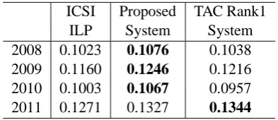
Table 1 shows the ROUGE-2 results of our pro-posed system, the ICSI system, and also the best performing system in the NIST TAC evaluation. We can see that our proposed system consistently outperforms ICSI ILP system (the gain is statis-tically significant based on ROUGE’s 95% confi-dence internal results). Compared to the best re-ported TAC result, our method has better perfor-mance on three data sets, except 2011 data. Note that the best performing system for the 2009 data is the ICSI ILP system, with an additional com-pression step. Our ILP method is purely
extrac-tive. Even without using compression, our ap-proach performs better than the full ICSI system. The best performing system for the 2011 data also has some compression module. We expect that af-ter applying sentence compression and merging, we will have even better performance, however, our focus in this paper is on the bigram-based ex-tractive summarization.
[image:4.595.318.515.179.264.2]ICSI Proposed TAC Rank1 ILP System System 2008 0.1023 0.1076 0.1038 2009 0.1160 0.1246 0.1216 2010 0.1003 0.1067 0.0957 2011 0.1271 0.1327 0.1344
Table 1: ROUGE-2 summarization results. There are several differences between the ICSI system and our proposed method. First is the bigrams (concepts) used. We use the top 100 bigrams from our bigram estimation module; whereas the ICSI system just used the initial bi-gram set described in Section 3.2. Second, the weights for those bigrams differ. We used the es-timated value from the regression model; the ICSI system just uses the bigram’s document frequency in the original text as weight. Finally, two systems use different ILP setups. To analyze which fac-tors (or all of them) explain the performance dif-ference, we conducted various controlled experi-ments for these three factors (bigrams, weights, ILP). All of the following experiments use the TAC 2009 data as the test set.
4.2 Effect of Bigram Weights
In this experiment, we vary the weighting methods for the two systems: our proposed method and the ICSI system. We use three weighting setups: the estimated bigram frequency value in our method, document frequency, or term frequency from the original text. Table 2 and 3 show the results using the top 100 bigrams from our system and the ini-tial bigram set from the ICSI system respectively. We also evaluate using the two different ILP con-figurations in these experiments.
# Weight ILP ROUGE-2
1
Estimated value Proposed 0.1246
2 ICSI 0.1178
3
Document freq Proposed 0.1109
4 ICSI 0.1132
5
Term freq Proposed 0.1116
[image:5.595.72.295.62.161.2]6 ICSI 0.1080
Table 2: Results using different weighting meth-ods on the top 100 bigrams generated from our proposed system.
# Weight ILP ROUGE-2
1
Estimated value Proposed 0.1157
2 ICSI 0.1161
3
Document freq Proposed 0.1101
4 ICSI 0.1160
5
Term freq Proposed 0.1109
6 ICSI 0.1072
Table 3: Results using different weighting meth-ods based on the initial bigram sets. The average number of bigrams is around 80 for each topic. the bigram’s term frequency is slightly more use-ful than its document frequency. This indicates that our estimated value is more related to bi-gram’s term frequency in the original text. When the weight is document frequency, the ICSI’s re-sult is better than our proposed ILP; whereas when using term frequency as the weights, our ILP has better results, again suggesting term frequency fits our ILP system better. When the weight is esti-mated value, the results depend on the bigram set used. The ICSI’s ILP performs slightly better than ours when it is equipped with the initial bigram, but our proposed ILP has much better results us-ing our selected top100 bigrams. This shows that the size and quality of the bigrams has an impact on the ILP modules.
4.3 The Effect of Bigram Set’s size
In our proposed system, we use 100 top bigrams. There are about 80 bigrams used in the ICSI ILP system. A natural question to ask is the impact of the number of bigrams and their quality on the summarization system. Table 4 shows some statis-tics of the bigrams. We can see that about one third of bigrams in the reference summary are in the original text (127.3 out of 321.93), verifying that people do use different words/bigram when
writing abstractive summaries. We mentioned that we only use the top-N (n is 100 in previous ex-periments) bigrams in our summarization system. On one hand, this is to save computational cost for the ILP module. On the other hand, we see from the table that only 127 of these more than 2K bi-grams are in the reference summary and are thus expected to help the summary responsiveness. In-cluding all the bigrams would lead to huge noise.
# bigrams in ref summary 321.93 # bigrams in text and ref summary 127.3 # bigrams used in our regression model 2140.7
(i.e., in selected sentences)
Table 4: Bigram statistics. The numbers are the average ones for each topic.
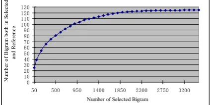
Fig 1 shows the bigram coverage (number of bi-grams used in the system that are also in reference summaries) when we varyN selected bigrams. As expected, we can see that as n increases, there are more reference summary bigrams included in the system. There are 25 summary bigrams in the top-50 bigrams and about 38 in top-100 bigrams. Compared with the ICSI system that has around 80 bigrams in the initial bigram set and 29 in the ref-erence summary, our estimation module has better coverage.
0 10 20 30 40 50 60 70 80 90 100 110 120 130
50 500 950 1400 1850 2300 2750 3200
Number of Selected Bigram
N
u
m
b
e
r
o
f
B
ig
ra
m
b
o
th
in
S
e
le
c
te
d
a
n
d
R
e
fe
re
n
c
[image:5.595.310.522.475.581.2]e
Figure 1: Coverage of bigrams (number of bi-grams in reference summary) when varying the number of bigrams used in the ILP systems.
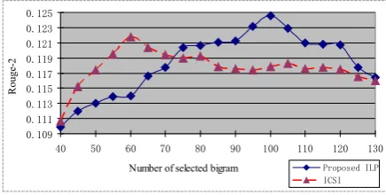
We can see that the ICSI ILP system performs better when the input bigrams have less noise (those bigrams that are not in summary). However, our proposed method is slightly more robust to this kind of noise, possibly because of the weights we use in our system – the noisy bigrams have lower weights and thus less impact on the final system performance. Overall the two systems have sim-ilar trends: performance increases at the begin-ning when using more bigrams, and after certain points starts degrading with too many bigrams. The optimal number of bigrams differs for the two systems, with a larger number of bigrams in our method. We also notice that the ICSI ILP system achieved a ROUGE-2 of 0.1218 when using top 60 bigrams, which is better than using the initial bigram set in their method (0.1160).
0.109 0.111 0.113 0.115 0.117 0.119 0.121 0.123 0.125
40 50 60 70 80 90 100 110 120 130
Number of selected bigram
R
o
u
g
e-2
[image:6.595.351.480.62.105.2]Proposed ILP ICSI
Figure 2: Summarization performance when vary-ing the number of bigrams for two systems.
4.4 Oracle Experiments
Based on the above analysis, we can see the impact of the bigram set and their weights. The following experiments are designed to demonstrate the best system performance we can achieve if we have ac-cess to good quality bigrams and weights. Here we use the information from the reference summary.
The first is an oracle experiment, where we use all the bigrams from the reference summaries that are also in the original text. In the ICSI ILP system, the weights are the document frequency from the multiple reference summaries. In our ILP module, we use the term frequency of the bigram. The oracle results are shown in Table 5. We can see these are significantly better than the automatic systems.
From Table 5, we notice that ICSI’s ILP per-forms marginally better than our proposed ILP. We hypothesize that one reason may be that many bi-grams in the summary reference only appear once. Table 6 shows the frequency of the bigrams in the summary. Indeed 85% of bigram only appear once
ILP System ROUGE-2
Our ILP 0.2124 ICSI ILP 0.2128
Table 5: Oracle experiment: using bigrams and their frequencies in the reference summary as weights.
and no bigrams appear more than 9 times. For the majority of the bigrams, our method and the ICSI ILP are the same. For the others, our system has slight disadvantage when using the reference term frequency. We expect the high term frequency may need to be properly smoothed/normalized.
Freq 1 2 3 4 5 6 7 8 9
[image:6.595.73.291.307.417.2]Ave# 277 32 7.5 3.2 1.1 0.3 0.1 0.1 0.04
Table 6: Average number of bigrams for each term frequency in one topic’s reference summary.
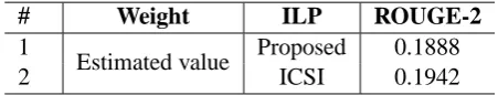
We also treat the oracle results as the gold stan-dard for extractive summarization and compared how the two automatic summarization systems differ at the sentence level. This is different from the results in Table 1, which are the ROUGE re-sults comparing to human written abstractive sum-maries at the n-gram level. We found that among the 188 sentences in this gold standard, our system hits 31 and ICSI only has 23. This again shows that our system has better performance, not just at the word level based on ROUGE measures, but also at the sentence level. There are on average 3 different sentences per topic between these two results.
summarization.
# Weight ILP ROUGE-2
1
Estimated value Proposed 0.1888
2 ICSI 0.1942
Table 7: Summarization results when using the es-timated weights and only keeping the bigrams that are in the reference summary.
4.5 Effect of Training Set
Since our method uses supervised learning, we conduct the experiment to show the impact of training size. In TAC’s data, each topic has two sets of documents. For set A, the task is a standard summarization, and there are 4 reference sum-maries, each 100 words long; for set B, it is an up-date summarization task – the summary includes information not mentioned in the summary from set A. There are also 4 reference summaries, with 400 words in total. Table 8 shows the results on 2009 data when using the data from different years and different sets for training. We notice that when the training data only contains set A, the perfor-mance is always better than using set B or the com-bined set A and B. This is not surprising because of the different task definition. Therefore, for the rest of the study on data size impact, we only use data set A from the TAC data and the DUC data as the training set. In total there are about 233 topics from the two years’ DUC data (06, 07) and three years’ TAC data (08, 10, 11). We incrementally add 20 topics every time (from DUC06 to TAC11) and plot the learning curve, as shown in Fig 3. As expected, more training data results in better per-formance.
Training Set # Topics ROUGE-2
[image:7.595.309.526.64.180.2]08 Corpus (A) 48 0.1192 08 Corpus( B) 48 0.1178 08 Corpus (A+B) 96 0.1188 10 Corpus (A) 46 0.1174 10 Corpus (B) 46 0.1167 10 Corpus (A+B) 92 0.1170 11 Corpus (A) 44 0.1157 11 Corpus (B) 44 0.1130 11 Corpus (A+B) 88 0.1140 Table 8: Summarization performance when using different training corpora.
0.112 0.113 0.114 0.115 0.116 0.117 0.118 0.119 0.12 0.121 0.122 0.123 0.124 0.125
20 40 60 80 100 120 140 160 180 200 220 240
Number of trainning topics
R
o
u
g
e
[image:7.595.70.296.89.132.2]-2
Figure 3: Learning curve
4.6 Summary of Analysis
The previous experiments have shown the impact of the three factors: the quality of the bigrams themselves, the weights used for these bigrams, and the ILP module. We found that the bigrams and their weights are critical for both the ILP se-tups. However, there is negligible difference be-tween the two ILP methods.
An important part of our system is the super-vised method for bigram and weight estimation. We have already seen for the previous ILP method, when using our bigrams together with the weights, better performance can be achieved. Therefore we ask the question whether this is simply because we use supervised learning, or whether our pro-posed regression model is the key. To answer this, we trained a simple supervised binary classifier for bigram prediction (positive means that a bi-gram appears in the summary) using the same set of features as used in our bigram weight estima-tion module, and then used their document fre-quency in the ICSI ILP system. The result for this method is 0.1128 on the TAC 2009 data. This is much lower than our result. We originally ex-pected that using the supervised method may out-perform the unsupervised bigram selection which only uses term frequency information. Further ex-periments are needed to investigate this. From this we can see that it is not just the supervised meth-ods or using annotated data that yields the over-all improved system performance, but rather our proposed regression setup for bigrams is the main reason.
5 Related Work
competitive performance for extractive summa-rization task. Maximum marginal relevance (MMR) (Carbonell and Goldstein, 1998) uses a greedy algorithm to find summary sentences. (Mc-Donald, 2007) improved the MMR algorithm to dynamic programming. They used a modified ob-jective function in order to consider whether the selected sentence is globally optimal. Sentence-level ILP was also first introduced in (McDon-ald, 2007), but (Gillick and Favre, 2009) revised it to concept-based ILP. (Woodsend and Lapata, 2012) utilized ILP to jointly optimize different as-pects including content selection, surface realiza-tion, and rewrite rules in summarization. (Gala-nis et al., 2012) uses ILP to jointly maximize the importance of the sentences and their diversity in the summary. (Berg-Kirkpatrick et al., 2011) applied a similar idea to conduct the sentence compression and extraction for multiple document summarization. (Jin et al., 2010) made a com-parative study on sentence/concept selection and pairwise and list ranking algorithms, and con-cluded ILP performed better than MMR and the diversity penalty strategy in sentence/concept se-lection. Other global optimization methods in-clude submodularity (Lin and Bilmes, 2010) and graph-based approaches (Erkan and Radev, 2004; Leskovec et al., 2005; Mihalcea and Tarau, 2004). Various unsupervised probabilistic topic models have also been investigated for summarization and shown promising. For example, (Celikyilmaz and Hakkani-T ¨ur, 2011) used it to model the hidden abstract concepts across documents as well as the correlation between these concepts to generate topically coherent and non-redundant summaries. (Darling and Song, 2011) applied it to separate the semantically important words from the low-content function words.
In contrast to these unsupervised approaches, there are also various efforts on supervised learn-ing for summarization where a model is trained to predict whether a sentence is in the summary or not. Different features and classifiers have been explored for this task, such as Bayesian method (Kupiec et al., 1995), maximum entropy (Osborne, 2002), CRF (Galley, 2006), and recently reinforce-ment learning (Ryang and Abekawa, 2012). (Aker et al., 2010) used discriminative reranking on mul-tiple candidates generated by A* search. Recently, research has also been performed to address some issues in the supervised setup, such as the class
data imbalance problem (Xie and Liu, 2010). In this paper, we propose to incorporate the supervised method into the concept-based ILP framework. Unlike previous work using sentence-based supervised learning, we use a regression model to estimate the bigrams and their weights, and use these to guide sentence selection. Com-pared to the direct sentence-based classification or regression methods mentioned above, our method has an advantage. When abstractive summaries are given, one needs to use that information to au-tomatically generate reference labels (a sentence is in the summary or not) for extractive summa-rization. Most researchers have used the similarity between a sentence in the document and the ab-stractive summary for labeling. This is not a per-fect process. In our method, we do not need to generate this extra label for model training since ours is based on bigrams – it is straightforward to obtain the reference frequency for bigrams by sim-ply looking at the reference summary. We expect our approach also paves an easy way for future au-tomatic abstractive summarization. One previous study that is most related to ours is (Conroy et al., 2011), which utilized a Naive Bayes classifier to predict the probability of a bigram, and applied ILP for the final sentence selection. They used more features than ours, whereas we use a discrim-inatively trained regression model and a modified ILP framework. Our proposed method performs better than their reported results in TAC 2011 data. Another study closely related to ours is (Davis et al., 2012), which leveraged Latent Semantic Anal-ysis (LSA) to produce term weights and selected summary sentences by computing an approximate solution to the Budgeted Maximal Coverage prob-lem.
6 Conclusion and Future Work
sets. From a series of experiments, we found that there is little difference between the two ILP mod-ules, and that the improved system performance is attributed to the fact that our proposed supervised bigram estimation module can successfully gather the important bigram and assign them appropriate weights. There are several directions that warrant further research. We plan to consider the context of bigrams to better predict whether a bigram is in the reference summary. We will also investigate the relationship between concepts and sentences, which may help move towards abstractive summa-rization.
Acknowledgments
This work is partly supported by DARPA under Contract No. HR0011-12-C-0016 and FA8750-13-2-0041, and NSF IIS-0845484. Any opinions expressed in this material are those of the authors and do not necessarily reflect the views of DARPA or NSF.
References
Ahmet Aker and Robert Gaizauskas. 2009. Summary generation for toponym-referenced images using ob-ject type language models. In Proceedings of the International Conference RANLP.
Ahmet Aker, Trevor Cohn, and Robert Gaizauskas. 2010. Multi-document summarization using a* search and discriminative training. In Proceedings of the EMNLP.
Taylor Berg-Kirkpatrick, Dan Gillick, and Dan Klein. 2011. Jointly learning to extract and compress. In Proceedings of the ACL.
Ronald Brandow, Karl Mitze, and Lisa F. Rau. 1995. Automatic condensation of electronic publications by sentence selection. Inf. Process. Manage.
Jaime Carbonell and Jade Goldstein. 1998. The use of mmr, diversity-based reranking for reordering docu-ments and producing summaries. In Proceedings of the SIGIR.
Asli Celikyilmaz and Dilek Hakkani-T¨ur. 2011. Dis-covery of topically coherent sentences for extractive summarization. In Proceedings of the ACL.
John M. Conroy, Judith D. Schlesinger, Jeff Kubina, Peter A. Rankel, and Dianne P. O’Leary. 2011. Classy 2011 at tac: Guided and multi-lingual sum-maries and evaluation metrics. In Proceedings of the TAC.
William M. Darling and Fei Song. 2011. Probabilistic document modeling for syntax removal in text sum-marization. In Proceedings of the ACL.
Sashka T. Davis, John M. Conroy, and Judith D. Schlesinger. 2012. Occams - an optimal combinato-rial covering algorithm for multi-document summa-rization. In Proceedings of the ICDM.
H. P. Edmundson. 1969. New methods in automatic extracting. J. ACM.
G¨unes Erkan and Dragomir R. Radev. 2004. Lexrank: graph-based lexical centrality as salience in text summarization. J. Artif. Int. Res.
Dimitrios Galanis, Gerasimos Lampouras, and Ion An-droutsopoulos. 2012. Extractive multi-document summarization with integer linear programming and support vector regression. In Proceedings of the COLING.
Michel Galley. 2006. A skip-chain conditional random field for ranking meeting utterances by importance. In Proceedings of the EMNLP.
Dan Gillick and Benoit Favre. 2009. A scalable global model for summarization. In Proceedings of the Workshop on Integer Linear Programming for Natu-ral Langauge Processing on NAACL.
Dan Gillick, Benoit Favre, and Dilek Hakkani-T¨ur. 2008. In The ICSI Summarization System at TAC 2008.
Feng Jin, Minlie Huang, and Xiaoyan Zhu. 2010. A comparative study on ranking and selection strate-gies for multi-document summarization. In Pro-ceedings of the COLING.
Julian Kupiec, Jan Pedersen, and Francine Chen. 1995. A trainable document summarizer. In Proceedings of the SIGIR.
Jure Leskovec, Natasa Milic-Frayling, and Marko Gro-belnik. 2005. Impact of linguistic analysis on the semantic graph coverage and learning of document extracts. In Proceedings of the AAAI.
Hui Lin and Jeff Bilmes. 2010. Multi-document sum-marization via budgeted maximization of submodu-lar functions. In Proceedings of the NAACL.
Chin-Yew Lin. 2004. Rouge: a package for auto-matic evaluation of summaries. In Proceedings of the ACL.
Ryan McDonald. 2007. A study of global inference al-gorithms in multi-document summarization. In Pro-ceedings of the European conference on IR research.
Rada Mihalcea and Paul Tarau. 2004. Textrank: Bringing order into text. In Proceedings of the EMNLP.
Dragomir R. Radev. 2001. Experiments in single and multidocument summarization using mead. In In First Document Understanding Conference.
Seonggi Ryang and Takeshi Abekawa. 2012. Frame-work of automatic text summarization using rein-forcement learning. In Proceedings of the EMNLP.
Noah A. Smith and Jason Eisner. 2005. Contrastive estimation: training log-linear models on unlabeled data. In Proceedings of the ACL.
Kristian Woodsend and Mirella Lapata. 2012. Mul-tiple aspect summarization using integer linear pro-gramming. In Proceedings of the EMNLP.