Learning and the effectiveness of central bank forward guidance

Munich Personal RePEc Archive

Learning and the effectiveness of central

bank forward guidance

Cole, Stephen

7 September 2015

Learning and the Effectiveness of Central Bank

Forward Guidance

Stephen J. Cole ∗

This version: September 7, 2015 First version: August 25, 2014

Abstract

The unconventional monetary policy of forward guidance operates through the management of expectations about future paths of interest rates. This paper examines the link between expectations formation and the effectiveness of forward guidance. A standard New Keynesian model is extended to include forward guidance shocks in the monetary policy rule. Agents form expectations about future macroeconomic variables via either the standard rational expecta-tions hypothesis or a more plausible theory of expectaexpecta-tions formation called adaptive learning. The results show the efficacy of forward guidance depends on the manner in which agents form their expectations. In response to forward guidance, the paths of the output gap and inflation under adaptive learning overshoot and undershoot those implied by rational expectations. The adaptive learning impulse responses of the endogenous variables to a forward guidance shock exhibit more persistence before and after the forward guidance shock has been realized upon the economy. During an economic crisis (e.g. a recession), the assumption of rational expecta-tions overstates the effects of forward guidance relative to adaptive learning. Specifically, the output gap is higher under rational expectations than adaptive learning. Thus, if monetary policy is based on a model with rational expectations, which is the standard assumption in the macroeconomic literature, the results of forward guidance could be potentially misleading.

Keywords: Forward Guidance, Monetary Policy, Adaptive Learning, Expectations.

JEL classification: D84, E30, E50, E52, E58, E60.

∗_{Department of Economics, Marquette University, P.O. Box 1881, Milwaukee, WI 53201. Phone: (414) 288-3367.}

1

Introduction

Once U.S. short-term interest rates effectively reached the zero lower bound (ZLB) during the

2007-2009 global financial crisis, monetary policymakers exhausted the conventional policy tool as

overnight interest rates could not be lowered. In response, central banks pursued “unconventional”

policies. One of these alternatives pursued by the Federal Reserve was large-scale asset purchases

(LSAPs) where the central bank purchases longer-term securities in hopes of lowering long-term

yields. Another unconventional policy was forward guidance, where the central bank communicates

to the public information about the future course of the policy rate. Forward guidance has been

pursued by central banks such as the Federal Reserve, Bank of Canada, Bank of England, and

the European Central Bank. An example of forward guidance was given in the September 2012

Federal Open Market Committee (FOMC) statement: “the Committee also . . . anticipates that

exceptionally low levels for the federal funds rate are likely to be warranted at least through

mid-2015.” In addition, Eggertsson and Woodford (2003) and Woodford (2012) argue that committing

to an interest rate path that is lower than what one would commit to under normal circumstances

(i.e. when overnight interest rates are away from the ZLB) can have additional stimulative economic

effects. Standard New Keynesian models (e.g. Woodford [2003]) predict consumption, investment,

and pricing decisions are sensitive to the expected path of short term interest rates. If agents expect

low interest rates in the future, current consumption and prices all increase. This stimulative effect

can be limited by a conventional monetary policy rule that adjusts interest rates in response to

target variables, such as the output gap and inflation. Households and firms may rationally expect

higher interest rates in response to future expansions. If a forward guidance statement, instead,

keeps a low policy rate through part of the expansion, consumption today will not be as limited.

The effectiveness of forward guidance hinges on how private sector expectations about

eco-nomic state variables (e.g. output and inflation) and interest rates respond to forward guidance.

Therefore, it is important to study whether the economic effects of forward guidance are sensitive to

the rational expectations assumption that is the standard benchmark in macroeconomic models.1

While a reasonable benchmark that is popular among macroeconomic models, rational expectations

makes strong assumptions about the amount of knowledge agents possess when forming beliefs. It

is natural then to examine how effective forward guidance policies can be under a more plausible

theory of expectations formation.

This paper studies the effectiveness of forward guidance in an environment where rational

1

expectations has been replaced by an adaptive learning rule similar to one proposed by Marcet and

Sargent (1989) and Evans and Honkapohja (2001). In particular, the economic environment is based

on Preston (2005) who derives a New Keynesian model with (potentially) non-rational expectations.

Households and firms formulate spending and pricing decisions, respectively, that depend on their

subjective expectations about future economic conditions and interest rates. The novelty of this

paper is to incorporate policy communication about future interest rates into agents’ subjective

expectations. The central bank sets interest rates according to a monetary policy rule that responds

positively to the output gap and inflation. The rule is augmented with anticipated shocks as in

Del Negro, Giannoni, and Patterson (2012) and Laseen and Svensson (2011).2 _{The anticipated}

shocks define central bank communication about future deviations from a normal interest rate rule

that agents know today. The shocks also represent time-contingent forward guidance in which the

central bank communicates a definitive forward guidance end date. In this case, communication

about the future path of interest rates is for a fixed amount of periods into the future and is

independent of economic conditions.3

Agents are assumed to form expectations via either the rational expectations hypothesis

or an adaptive learning rule. The former is a strong assumption and assumes agents construct

expectations with respect to the true probability distribution of the model. Rational expectations

agents must know the model’s deep parameters, structure of the model, beliefs of other agents,

and distribution of the error terms. A popular alternative to rational expectations is adaptive

learning. This approach builds from the cognitive consistency principle that agents behave as

real-life economists (see, for instance, Evans and Honkapohja [2013]). An econometrician, for example,

would produce forecasts of future economic variables by forming an econometric model. He or she

would estimate the parameters using standard econometric techniques. As new data arrives, these

forecasts would be revised. Thus, a real-life economist is engaging in a process of learning about

the economy. Analogously, adaptive learning agents are assumed to behave as econometricians and

formulate forecasts of future endogenous variables using standard econometric techniques. The

variables in their econometric model are based on the solution found under rational expectations,

but adaptive learning agents estimate the parameters using ordinary least squares. Their beliefs

about future endogenous variables are appropriately revised as new data arrive.4

2

The anticipated shocks are similar to the news shocks of Schmitt-Groh´e and Uribe (2012).

3

This type of forward guidance is in contrast to state-contingent forward guidance where the duration of a constant interest rate path is linked to economic conditions.

4

The results of this paper show that the desired effect of forward guidance depends on the

man-ner in which agents form their expectations. This outcome is first shown during normal economic

times.5 The impulse responses of the endogenous variables under adaptive learning fail to capture

the precise effects a forward guidance shock has on the economy. There exists more persistence

in the paths of the output gap and inflation under adaptive learning than rational expectations.

Differences also occur when the central bank communicates to both rational expectations and

adap-tive learning agents the same forward guidance information such that the interest rate will equal

zero for an extended period of time. The output gap and inflation return to long-run equilibrium

quicker under rational expectations than adaptive learning. Under adaptive learning, the paths of

the output gap and inflation overshoot and undershoot the rational expectations paths.

Conse-quently, there exists larger variation of the paths of the output gap and inflation under adaptive

learning than rational expectations. These effects occur because rational expectations agents fully

understand the precise and positive effects of forward guidance on the economy. However,

adap-tive learning agents fail to understand the posiadap-tive effects and must continually make adjustments

to their beliefs causing them to overshoot and undershoot the rational expectations paths of the

output gap and inflation.

The effectiveness of forward guidance is also examined under a period of economic crisis (e.g.

a recession). The policy experiment includes a scenario where forward guidance is implemented to

combat the effects of a downturn in the economy. The results show the effects of forward guidance

under rational expectations are overstated relative to adaptive learning. Specifically, the value of

the output gap is higher under the assumption of rational expectations than adaptive learning.

The reason is that rational expectations agents base their expectations of future values of the

endogenous variables on the true model of the economy. They understand the economic downturn

and how forward guidance will precisely alleviate the economy. However, adaptive learning agents

observe the economic downturn, but fail to fully understand how forward guidance will improve the

economy. They are estimating the effects of forward guidance on the economy as their forecasts

are based on an econometric model.

Overall, the results of the paper suggest a main finding: policymakers should exercise caution

when recommending forward guidance policy. If monetary policy is based on a model with the

standard rational expectations hypothesis, which assumes agents know the true structure of the

model, the results may be misleading relative to a more plausible theory of expectations formation

(e.g. adaptive learning). Specifically, during an economic crisis, the predicted effects of forward

5

guidance under the rational expectations assumption are overstated in comparison to adaptive

learning.

1.1 Previous Literature

This paper contributes to the growing literature on unconventional monetary policy. Eggertsson

and Woodford (2003) explain that the expectations channel plays a key role on the economy when

interest rates are at the ZLB and at any level. Specifically, they describe that the future path of

short-term interest rates affects long-term interest rates and asset prices, and thus, the management

of expectations about future interests rates affects agents’ optimal decisions. De Graeve, Ilbas, and

Wouters (2014) find that the effectiveness of forward guidance does not necessarily work through

decreasing the long-run interest rate, contrary to previous studies. The type of forward guidance

and lack of information about the underlying reasons for implementing forward guidance (e.g.

monetary stimulus or sign of future economic crisis) can dampen the effects of this monetary policy

tool. Levin, L´opez-Salido, Nelson, and Yun (2010) explain that the efficacy of forward guidance

can vary with the type of structural shock affecting the economy. In addition, recent literature

has found large effects from forward guidance. Carlstrom, Fuerst, and Paustian (2012) show that

standard New Keynesian models with the interest rate fixed for a finite period of time result in

extreme responses of output and inflation. McKay, Nakamura, and Steinsson (2015) explain that

the extraordinary responses to forward guidance predicted by standard macroeconomic models are

sensitive to the assumption of complete markets. The effectiveness of forward guidance at the

ZLB is reduced when precautionary savings are added into a macroeconomic model. Del Negro

et al. (2012) construct a Dynamic Stochastic General Equilibrium (DSGE) model with forward

guidance, which produces large responses of macroeconomic variables to forward guidance. Del

Negro et al. (2012) state that the long-term bond yield drives these unusually high responses. As

will be discussed in Section 4.3, this current paper suggests that the exceedingly large responses to

forward guidance found in the previously mentioned articles could be due to the manner in which

expectations are modeled.

The model in this paper utilizes time-contingent forward guidance since there has been recent

evidence of its effectiveness. G¨urkaynak, Sack, and Swanson (2005) find empirical evidence that

FOMC statements about the future path of the policy rate greatly contribute to the changes in

the long-term interest rates. Swanson and Williams (2014) show that Federal Reserve forward

guidance announcements affect market expectations about future policy. Woodford (2012) also

rate swaps (OIS) to measure market expectations about the policy rate in Canada, Woodford

(2012) displays that OIS rates immediately changed upon release of the Bank of Canada’s forward

guidance statement. The work of Chang and Feunou (2013) show that the Bank of Canada’s

forward guidance statement in 2009 had positive effects on the economy by reducing uncertainty

about future monetary policy rates. A reduction in interest rate uncertainty can affect levels

of investment, output, and unemployment in the economy as described by Baker, Bloom, and

Davis (2013). Femia, Friedman, and Sack (2013) show evidence that financial variables, such

as Treasury yields and equity prices, reacted favorably to the Federal Reserve’s time-contingent

forward guidance announcements.

By analyzing the role of expectations formation on forward guidance, this paper builds on the

adaptive learning and policy literature. Mitra, Evans, and Honkapohja (2012) examine the effects

of the fiscal authority giving guidance on the future course of government purchases and taxes. The

results show that a temporary change in fiscal policy leads to different effects on adaptive learning

and rational expectations agents. The adaptive learning output multipliers seem to match empirical

data more than its rational expectations counterparts. Eusepi and Preston (2010) investigate the

link between adaptive learning and central bank communication strategies. Increased central bank

communication, such as communicating the monetary policy rule and the variables within the rule,

can lead to increased macroeconomic stability. Preston (2006) studies forecast-based monetary

policy rules and adaptive learning. He finds that a central bank that understands the basis of

private sector forecasts can aid in increasing macroeconomic stability.

The remaining sections of the paper are organized as follows. Section two presents the New

Keynesian model with forward guidance. Section three discusses expectations formation under

both rational expectations and adaptive learning. Section four presents the outcomes of forward

guidance under both rational expectations and adaptive learning. Section five examines the results

under different parameter schemes. Section six concludes.

2

Model

The aggregate dynamics of the economy are described by a New Keynesian model derived under

(potentially) non-rational expectations (see Preston [2005]). There exists a continuum of households

indexed byi∈[0,1]. Households maximize expected future discounted utility

ˆ

Ei t

∞

X

T=t

βT−t

U(C_Ti;ξT)−

Z 1

0

v(hi_T(j);ξT)dj

whereβ is the discount factor and is bounded between zero and one. Utility depends onCi

T, which

is consumption by householdi of goods in the economy. Households also receive a disutility when

supplying labor, hi

T(j), for the production of each good j. ξT denotes an aggregate preference

shock. ˆEi

t denotes (potentially) non-rational expectations that satisfy standard probability laws,

such as ˆEi

tEˆt+1i = ˆEti. Beliefs are assumed to be homogeneous across agents, but agents do not

know this fact.

A household is subject to a budget constraint that takes the following form

M_ti+Bi_t≤(1 +im_t−1)M i

t−1+ (1 +it−₁)B_ti−1+PtY i

t −Tt−PtCti (2)

whereTtdenotes lump-sum taxes and transfers,Mtiis money holdings, andimt denotes interest paid

on money balances. Asset markets are assumed to be incomplete such that household’s can transfer

wealth between periods through a one-period riskless bond Bi

t. Accordingly,it is the interest paid

on bonds. Yi

t is household i’s real income. Pt is the aggregate price index, and PtYti denotes

householdi’s nominal income which is given by

PtYti =

Z 1

0

[wt(j)hit(j) + Πt(j)]dj (3)

A household receives wageswt(j) for hours worked towards the production of goodj,hit(j). Since

each household owns an equal part of each firm, it receives profits from the sale of good j, Πt(j).

Furthermore, even though it is present in the budget constraint, money does not show up in the

utility function. It is assumed that money balances do not relieve any transactional frictions.

However, a household may choose to hold money balances because it provides a financial return.

The aggregate variablesCi

t and Pt are assumed to be defined by the Dixit-Stiglitz

constant-elasticity-of-substitution aggregator

Cti ≡

Z 1

0

cit(j)

θ−1

θ dj

θ θ−1

(4)

Pt ≡

Z 1

0

pt(j)1 −θ_dj

1 1₋θ

(5)

whereθ >1 is the elasticity of substitutions across differentiated goods, ci

t(j) describes household

i’s consumption of goodj, and pt(j) is the price of goodj.

By log-linearizing the intertemporal budget constraint and Euler equation, the following

results are obtained

ˆ Ei t ∞ X T=t

βT−t_Cˆi

T = w¯ti+ ˆEti ∞

X

T=t

βT−t_Yˆi

T (6)

ˆ

Ci

t = EˆtiCˆ i

where ˆπt is current inflation, σ ≡ _U−Uc

ccC¯ defines the intertemporal elasticity of substitution, gt ≡

σUcξξt

Uc denotes a preference shock, and ¯w

i

t≡

Wi t

PtY¯ is share of real wealth (W

i

t ≡(1 +it−₁)B_ti−₁) as a

fraction of steady-state income. The “ ˆ ” symbol over variables denotes log deviations from steady

state. By solving (7) backwards from dateT tot, taking expectations at timet, plugging the result

into (6), and integrating overi, the following equation for aggregate consumption emerges

ˆ

Ct= ˆEt ∞

X

T=t

βT−th_{(1−β) ˆY}

T −βσ(ˆiT −πˆT+1) +β(gT −gT+1)

i

(8)

Note that R_iw¯i

tdi = 0 since bonds are in zero net supply from market clearing. Eˆt =

R

iEˆtidi

denotes the average expectations operator. By imposing the market equilibrium condition ˆYt= ˆCt

and defining the resulting equation in terms of the output gap ˆxt≡Yˆt−Yˆtn, the following equation

emerges

ˆ

xt = Eˆt ∞

X

T=t

βT−t_[(1−β)ˆx

T+1−σ(ˆiT −πˆT+1) + ˆrnT] (9)

where

ˆ

rn

t = ρnrˆnt−₁+ε n

t (10)

andεn t

iid

∼N(0, σ_n2). ˆYn

t is the natural rate of output, that is, output prevailing under flexible prices,

and ˆrn

t ≡( ˆYt+1n −gt+1)−( ˆYtn−gt). Equation (9) relates the current output gap ˆxt to current and

future expected values of the output gap, interest rate ˆit, inflation rate ˆπt, and natural real interest

rate shock ˆrn

t. Households take into account the future values of the endogenous variables infinitely

far into the future when choosing optimal consumption today. Intuitively, the expected course of

a household’s consumption pattern matters to its optimal consumption today. A household also

knows future consumption patterns are affected by future values of income, interest rates, and

inflation. Thus, expectations of these variables are important for decisions today.

The production side of the economy is populated by firms that operate in a monopolistically

competitive environment. Each good is produced using labor from households. A firm is subject

to a Calvo (1983) pricing scheme. Each period a fraction 0<1−α <1 of producers can optimally

reset their prices. The remaining α producers retain the same prices from the previous period.

Furthermore, a good is produced following the production functionyt(i) =Atf(ht(i)) where At is

a technology shock. The demand curve for goodiis given byyt(i) =Yt(pt(i)/Pt)−θ. The following

Dixit-Stiglitz aggregate price index is assumed

Pt=

h

αP1−_θ

t−₁ + (1−α)p ∗₁−_θ t

i 1 1₋θ

A firm maximizes its expected present discounted value of profits ˆ Ei t ∞ X T=t

αT−_t

Qt,T[ΠiT(pt(i))] (12)

where Qt,T describes the stochastic discount factor showing how firms value its future stream of

income. The stochastic discount factor is given by

Qt,T =βT −_tPt

PT

Uc(YT, ξT)

Uc(Yt, ξt)

(13)

The profit function is defined by

Π_Ti (pt(i)) =YtPtθpt(i)1−θ−wt(i)f−1(YtPtθpt(i)−θ/At) (14)

Maximizing (12) with respect to pt(i) yields the following first order condition

ˆ

Eti ∞

X

T=t

αT−_t

Qt,TYTPTθ[ˆp ∗

t(i)−µP¯ Tst,T(i)] = 0 (15)

where ¯µ= _θ−θ₁, andst,T is the firm’s real marginal cost function. Furthermore, by substituting in

the stochastic discount factor and real marginal costs into the firm’s first order condition and then

log linearizing around a zero inflation steady state, the following result is produced

ˆ

p∗

t(i) = ˆEti ∞

X

T=t

(αβ)T−t

1−αβ

1 +ωθ(ω+σ

−1

)ˆxT +αβπˆT+1

(16)

ω defines the elasticity of a firm’s real marginal cost function with respect to its output and θ

measures the elasticity of substitution between differentiated goods. Note also that log linearizing

(11) yields

ˆ

πt= ˆp ∗

t(1−α)/α (17)

where ˆπt is current inflation. Integrating over i and plugging (17) into (16) yields the following

equation for inflation

ˆ

πt = κxˆt+ ˆEt ∞

X

T=t

(αβ)T−t_[καβxˆ

T+1+ (1−α)βπˆT+1+ ˆµT] (18)

where

ˆ

µt = ρµµˆt−₁+ε µ

t (19)

and εµ_t iid∼ N(0, σ2

µ).6 Equation (18) defines the inflation rate as a function of current and future

values of the output gap, inflation rate, and cost-push shock ˆµt. ωdescribes the elasticity of a firm’s

6

real marginal cost function with respect to its own output, andκ≡ (1−_αα)(1_(1+ωθ)−αβ)(ω+σ−₁

)>0. The

optimal decisions by firms are shown to depend on the long-run expected path of macroeconomic

variables because of the assumption of sticky prices. A firm must be concerned that it will not be

able to adjust its price in future periods regardless of future economic conditions. Thus, optimal

pricing decisions today require firms to forecast future states and values of economic variables.7

The model is closed by describing the central bank of the economy. The central bank follows

a monetary policy rule that takes the following form

ˆ_{it=χππˆt+χxxˆt+ε}M P

t +

L

X

l=1

εR_l,t−_l (20)

The short-term nominal interest rate changes based on the output gap, inflation rate, monetary

policy shock, and forward guidance shocks. εM P

t defines an unanticipated monetary policy shock

and is i.i.d. In order to incorporate forward guidance into the model, the monetary policy rule

is augmented with anticipated shocks following Del Negro et al. (2012) and Laseen and Svensson

(2011). Each anticipated or forward guidance shock (εl,t−l) is contained in the last term in equation

(20) and is i.i.d. Intuitively, the forward guidance shock can be thought of as an announcement

by the central bank in period t−l that the interest rate will change l periods later, i.e. in period

t. If the central bank has been communicating guidance on the interest rate for L periods ahead,

there would be 1,2,3, . . . , L forward guidance shocks that affect the monetary policy rule in period

t. Thus, L corresponds to the length of the forward guidance horizon announced by the central

bank. The last term in equation (20) can also be thought of as the sum of all forward guidance

commitments stated by the central bank 1,2, ..., andLperiods ago that affect the nominal interest

rate in period t. Following Del Negro et al. (2012) and Laseen and Svensson (2011), the system is

also augmented with L state variables v1,t, v2,t, ..., vL,t. The law of motion for each of these state

variables is given by

v1,t = v2,t−₁+εR_1,t (21)

v2,t = v3,t−₁+εR_2,t (22)

v3,t = v4,t−1+εR_3,t (23)

.. .

vL,t = εRL,t (24)

7

In other words, each component of vt = [v1,t, v2,t, ..., vL,t]′ is the sum of all central bank forward

guidance commitments known in period t that affect the interest rate 1,2, ..., and L periods into

the future, respectively.8 It should be noted that equations (21)−(24) can be simplified to find that

v1,t−₁ =

PL

l=1εRl,t−_l. In addition, equations (20)−(24) provide a computationally tractable method

to model forward guidance. Since the forward guidance shocks in equation (20) equal v1,t−1, the

forward guidance shocks can be put into a vector of predetermined variables in standard state-space

form. As described by Laseen and Svensson (2011), standard solution techniques then can be used

to solve the final system of equations. Another reason to model forward guidance in this way is that

it relieves the concern of the existence of multiple solutions. As described in Honkapohja and Mitra

(2005) and Woodford (2005), indeterminacy can arise if forward guidance is instead modeled as

pegging the interest rate to a certain value.9 For instance, without a monetary policy that responds

to economic fluctuations, real disturbances to the economy can produce a multitude of equilibrium

responses of the endogenous variables.

The following example presents the case where the central bank’s forward guidance horizon

is 2 periods ahead, i.e. L= 2. The model’s system of equations consists ofv1,t andv2,t whose laws

of motion are defined as

v1,t = v2,t−₁+εR_1,t =εR_2,t−₁+ε R

1,t (25)

v2,t = εR2,t (26)

Thus, v_1,tR defines the sum of all forward guidance commitments by the central bank known in

period t that affect the interest rate one period later. vR

1,t consists of current period forward

guidance affecting the interest rate one period later, εR

1,t, and previous period’s forward guidance

affecting the interest rate two periods later, v2,t−₁ =εR_2,t−₁. v2,t is the sum of all forward guidance

commitments by the central bank known in periodtthat affect the interest rate two periods later.

Since the forward guidance horizon is two periods,v2,t consists of current period forward guidance

affecting the interest rate two periods later, εR 2,t.10

The ZLB on interest rates is also enforced. Forward guidance has gained attention due to

interest rates effectively reaching the ZLB because of the 2007-2009 global financial recession. Thus,

8

In the terminology of Laseen and Svensson (2011),v1,t, v2,t, ..., vL,t are described as central bank “projections”

(p. 10) of whatPL_l=1ε

R

l,t−lwill be 1,2, ..., andLperiods into the future, respectively.

9

Carlstrom, Fuerst, and Paustian (2012) show that determinacy can arise from an interest rate peg if terminal conditions are known and a standard monetary policy rule is followed after the interest rate peg. However, unusually large responses of the output and inflation are found through this process.

10

it seems natural to model the ZLB on nominal interest rates when simulating forward guidance.

Specifically, equations (9) and (20) become

ˆ

xt = Eˆt ∞

X

T=t

βT−t_[(1−β)ˆx

T+1−σ(iT −i ∗

−πˆT+1) + ˆrTn] (27)

it = max{i∗+χππˆt+χxxˆt+εM Pt + L

X

l=1

εR_l,t−l,0} (28)

wherei∗

=r∗

+π∗

is the steady-state nominal interest rate.11

To summarize, the aggregate dynamics of the economy with forward guidance are defined

by the output gap, inflation rate, AR(1) shock processes, monetary policy rule with forward

guidance, and the laws of motion of the sum of central bank commitments, that is, equations

(9),(10),(18),(19), and (20)−(24). With enforcement of the ZLB, equations (27) and (28) are

used instead of (9) and (20). To simplify notation, the “ ˆ ” symbol over the variables is removed

for the remainder of the paper.

3

Expectation Formation

This paper assumes agents form expectations following either the rational expectations hypothesis

or adaptive learning. The difference between the two types of expectations formation regards

the amount of knowledge agents hold about the economy (See, for example, Marcet and Sargent

(1989), Evans and Honkapohja (2001), and Evans, Honkapohja, and Mitra (2009).). Under rational

expectations, agents know the structure of the model, parameters of the model (e.g. σ, κ, etc.),

distribution of the error terms, and beliefs of other agents. They compute expectations based

off the true model of the economy. Under adaptive learning, agents do not know the true model

of the economy, and thus, cannot compute precise expectations as under rational expectations.

Instead, they operate as econometricians by forming an econometric model to forecast values of

the endogenous variables. Their model includes the variables in the rational expectations solution.

Adaptive learning agents estimate the values of the model’s parameters using standard econometric

methods. As new information becomes available every period, they appropriately adjust their

forecasts.

Rational Expectations–The model defined by equations (9),(10),(18),(19), and (20)−(24)

can be simplified under the assumption of rational expectations. Agents with rational expectations

understand the beliefs of other agents and are able to compute the aggregate probabilities of the

model. As shown in Preston (2005), this additional information simplifies the infinite horizon

11

In a zero steady-state inflation rate,π∗_{= 0. The model implied steady-state real interest rater}∗_=β−1

model to the “benchmark” one step ahead New Keynesian model. Specifically, equations (9) and

(18) become

xt = Etxt+1−σ(it−Etπt+1) +rnt (29)

πt = βEtπt+1+κxt+µt (30)

The model with rational expectations can be solved using standard techniques, such as one

suggested by Sims (2002). The model can be written in general state-space form as suggested by

Sims (2002). This form is defined as

e

Γ0Yet=C+eΓ1Yet−₁+Γe₂eǫ_t+Γe₃ζ_t (31)

where

e

Yt = [xt, πt, it, rnt, µt, v1,t, v2,t, . . . , vL,t, Etxt+1, Etπt+1] ′

(32)

e

ǫt = [εnt, ε µ t, ε

M P

t , εR1,t, εR2,t, . . . , εRL,t] ′

(33)

C defines a vector of constants of required dimensions. ζtdefines the vector of expectational errors

(e.g. ζπ

t =πt−Et−1πt) of required dimensions. Using standard techniques to solve the model with

rational expectations (e.g. Sims [2002]) and the parameter values in Table 1, the solution to the

system under rational expectations is

e

Yt=Ce+ξ1Yet−₁+ξ₂eǫt (34)

where the matricesCe,ξ1, and ξ2 are defined in Appendix A.12

Adaptive Learning–In order to evaluate the expectations in equations (9) and (18) under

adaptive learning, agents act as econometricians by forming a model based on variables that

ap-pear in the rational expectations solution and estimate the coefficients. This model is labeled the

“Perceived Law of Motion” (PLM) and is constructed from the minimum state variable (MSV)

solution that exists under rational expectations.13 The PLM is defined as

Yt=a+bvt+cwt+dv1,t−₁+εt (35)

where

Yt = [xt, πt, it] ′

(36)

vt = [v1,t, v2,t, ..., vL,t] ′

(37)

12

Discussion of the parameter values can be found in Table 1 in Section 4.1.

13

The vector wt= [rnt, µt] ′

is defined by

wt=φwe t−₁+ ¯ε_t (38)

where

e

φ =

ρn 0

0 ρµ

(39)

¯

εt = [εnt, ε µ t]

′

(40)

By rewriting equations (21)−(24), the vector vt becomes

vt = Φvt−₁+ηt (41)

where

ηt = [εR1,t, . . . , εRL,t] ′

(42)

and Φ is anL xL matrix given by

Φ =           

0 1 0 0 . . . 0 0

0 0 1 0 . . . 0 0

0 0 0 1 . . . 0 0

..

. . .. ...

0 0 0 0 . . . 1 0

0 0 0 0 . . . 0 1

0 0 0 0 . . . 0 0

           (43) (44)

a,b,c, and dare unknown coefficient matrices of appropriate dimensions that agents estimate and

learn about over time.14 Furthermore, the addition ofv1,t−₁ is a necessary component of the PLM

since it is present in the rational expectations solution shown in AppendixA and not contained in

the vectorvt.15

An important component of adaptive learning models regards the information available to

agents when they form expectations. In this paper, adaptive learning agents are assumed to know

the values of the regressors in the PLM and previous period’s coefficient estimates when

form-ing beliefs about the future. They update their parameter estimates at the end of the period.

This assumption avoids the simultaneous determination of current period coefficient estimates and

14

In the PLM, the time subscript is left off the coefficients to emphasize that adaptive learning agents believe current period forecasts are optimal and do not take into account they will be updating their beliefs every period. However, as will be described later, the PLM coefficients will evolve over time.

15

Since this paper restricts attention to fundamentals solutions andYt−1 does not appear in equations (9), (18),

endogenous variables when forming expectations and making optimal decisions.16 _{The i.i.d.}

mon-etary policy shock is also assumed to be unobserved.17 Furthermore, the following is the timeline

of events:

1. At the beginning of period t, vt, and wt are observed by the agents and added to their

information set.

2. Agents use vt,wt, and v1,t−1 as well as previous period’s estimates (i.e. at−1,bt−1,ct−1, and

dt−₁) to form expectations about the future.

3. Yt is realized.

4. In order to update their parameter estimates, agents compute a least squares regression ofYt

on 1, vt,wt, and v1,t−₁.

Agents update their parameter estimates of the PLM by following the recursive least squares

(RLS) formula

φt = φt−1+τtR −₁

t zt(Yt−φ ′ t−₁zt)

′

(45)

Rt = Rt−₁+τt(ztz ′

t−Rt−₁) (46)

where φ = (a, b, c, d)′ contains the PLM coefficients to be estimated. Rt defines the precision

matrix of the regressors in the PLM zt ≡ [1, vt, wt, v1,t−₁] ′

. τt is known as the “gain” parameter

and controls the response of φt to new information. The last expression in equation (45) defines

the recent prediction error of the endogenous variables.

The gain parameter in equations (45) and (46) can either decrease over time or be fixed at

certain values. In the decreasing gain or RLS case, τt = t−1 and past observations are equally

weighted. Evans and Honkapohja (2001) explain that as t → ∞ the coefficients in the PLM

converge to the rational expectations coefficients with probability one. As is assumed in this

current paper, the gain parameter can also be fixed at a certain value. Under this method called

discounted or constant gain learning (CGL),τt= ¯τ and the most recent observations play a larger

role when updating agents’ coefficients and expectations. Evans and Honkapohja (2001) describe

that the coefficients in the PLM converge in distribution to their rational expectations values with

a variance that is proportional to the constant gain parameter. CGL may be a more realistic way

16

An alternative is to assume that agents use the coefficient estimates from the current period when forming expectations. This results in expectations and current period parameter estimates determined simultaneously when making optimal decisions.

17

to model learning since it allows agents to update their beliefs every period to new information as

a real-life econometrician revising his or her forecasts every period.

Agents solve for ˆEtYT+1 by using equation (35). For any T ≥ t, their expectations infinite

periods ahead are given by

ˆ

Et ∞

X

T=t

βT−t_Y

T+1= ˆEt ∞

X

T=t

βT−t_a

t−1+ ˆEt ∞

X

T=t

βT−t_b

t−1vT+1

+ ˆEt ∞

X

T=t

βT−_t

ct−₁w_T+1+ ˆE_t ∞

X

T=t

βT−_t

dt−₁v_1,T

(47) ˆ Et ∞ X T=t

(αβ)T−t_Y

T+1 = ˆEt ∞

X

T=t

(αβ)T−t_a

t−₁+ ˆEt ∞

X

T=t

(αβ)T−t_b

t−₁vT+1

+ ˆEt ∞

X

T=t

(αβ)T−_t

ct−1wT+1+ ˆEt ∞

X

T=t

(αβ)T−_t

dt−1v1,T

(48)

By noting the geometric sums and expectations ofvttwelve periods ahead or greater equal the zero

vector, equations (49) and (50) simplify to equal

ˆ

Et ∞

X

T=t

βT−_t

YT+1 = (1−β)−1at−1+bt−1Φ(IL−βΦ) −₁

(IL−(βΦ)11)vt

+ct−₁(I₂−βφe) −₁e

φwt+dt−₁[1, β, β2, . . . , β11]vt

(49) ˆ Et ∞ X T=t

(αβ)T−t_Y

T+1= (1−αβ)−1at−₁+b_t−₁Φ(I_L−αβΦ) −₁

(IL−(αβΦ)11)vt

+ct−₁(I₂−αβφe) −1e

φwt+dt−₁[1, αβ,(αβ)2, . . . ,(αβ)11]vt

(50)

Equations (49) and (50) are substituted into equations (9) and (18) to give

Yt= Γ0(φt−1) + Γ1(φt−1)Yt−1+ Γ2(φt−1)vt+ Γ3(φt−1)wet (51)

where

e

wt= [wt, εM Pt ] ′

(52)

Equation (51) is called the “Actual Law of Motion” (ALM) and describes the actual evolution of

the endogenous variables implied by the PLM (35).

4.1 Parameterization

This section details the calibration values for the model’s parameters, which are shown in Table

1. The discount rate, β, is set to equal 0.99 which is a common value found in the literature.

The parameter representing the intertemporal elasticity of substitution is fixed at one. This value

has been assumed a priori in Smets and Wouters (2003). κ is set to equal 0.1. This number

roughly corresponds to a high degree of price stickiness, α, found in empirical work by Klenow

and Malin (2010), a value ofω found in Giannoni and Woodford (2004), and a value of θ found in

the literature (e.g. Gertler and Karadi [2011]). Monetary policy positively responds to the output

gap, and positively adjusts at more than a one-to-one rate to the inflation rate. χx= 0.125 follows

from Branch and Evans (2013). The value of χπ closely follows empirical adaptive learning work

by Milani (2007). The structural disturbances are not assumed to exhibit high persistence. The

distribution of the white noise shocks is not assumed to be highly dispersed. There also is no

covariance between the structural shocks.

The current paper examines results for the CGL case. In regards to choosing the CGL

parameter ¯τ, this paper uses 0.02. This choice is close to the results used in the literature, such

as Orphanides and Williams (2005), Milani (2007), and Branch and Evans (2006). For robustness,

the current methodology also examines the results under different values of ¯τ.

The value for the length of the forward guidance horizonLis chosen to match time-contingent

forward guidance by the Federal Reserve. This is based off the FOMC September 2012

state-ment:“the Committee also decided today to keep the target range for the federal funds rate at 0

to 1/4 percent and currently anticipates that exceptionally low levels for the federal funds rate are

likely to be warranted at least through mid-2015.” This announcement was one of the last FOMC

statements to exclusively use time-contingent forward guidance language. By taking “mid-2015”

to be at most the end of the third quarter of 2015, the number of quarters from September 2012

to “mid-2015” is twelve. Thus,L= 12.

4.2 Normal Economic Times

4.2.1 Impulse Responses

In this section, impulse responses of the output gap and inflation rate to negative one unit

mone-tary policy and forward guidance shocks under different expectation assumptions are examined in

Figures 1 and 2.18 The forward guidance shocks are the anticipated shocks found in equations (21)

- (24). Since equation (51) exhibits a nonlinear structure, standard linear techniques to compute

18

Table 1: Parameter Values

Description Value

σ IES 1

β Discount Factor 0.99

κ Function of Price Stickiness 0.1

α Price Stickiness 0.75

χπ Feedback Inflation 1.4

χx Feedback Output Gap 0.125

ρn Autoregressive Demand 0.5

ρµ Autoregressive Cost-Push 0.5

σn Demand Shock 0.001

σµ Cost-Push Shock 0.001

σi M.P Shock 0.001

σ1,i 1 Period Ahead FG Shock 0.001

σ2,i 2 Period Ahead FG Shock 0.001

σ3,i 3 Period Ahead FG Shock 0.001

σ4,i 4 Period Ahead FG Shock 0.001

σ5,i 5 Period Ahead FG Shock 0.001

σ6,i 6 Period Ahead FG Shock 0.001

σ7,i 7 Period Ahead FG Shock 0.001

σ8,i 8 Period Ahead FG Shock 0.001

σ9,i 9 Period Ahead FG Shock 0.001

σ10,i 10 Period Ahead FG Shock 0.001

σ11,i 11 Period Ahead FG Shock 0.001

σ12,i 12 Period Ahead FG Shock 0.001

L FG Horizon 12

¯

τ CGL 0.02

Note: FG stands for forward guidance.

impulse responses under adaptive learning do not apply. To remedy this situation, this paper

fol-lows Eusepi and Preston (2011) by proceeding in the following manner. The model is simulated

twice forT+K periods, where K is the impulse response function horizon. The impulse responses

are calculated starting in periodT+ 1.19 _{In the first simulation, time periodT+ 1 includes a}

neg-ative one unit shock. The K-period impulse response function is given by the difference between

the first and second simulations over the final K periods. The process is then repeated for 5,000

simulations and the mean impulse response across the 5,000 simulations is calculated to arrive at

the final impulse response trajectory. The impulse response function horizon is chosen to be twenty

periods, that is,K = 20.

Impact–As seen in Figures 1 and 2, the initial response of the macroeconomic variables is

approximately the same under both adaptive learning and rational expectations. This result is not

surprising since Evans and Honkapohja (2001) state that CGL coefficients converge to a Normal

19

0 2 4 6 8 10 12 14 16 18 20 −0.2

0 0.2 0.4 0.6 0.8 1 1.2 1.4

Output

ε_tMP

0 2 4 6 8 10 12 14 16 18 20 −0.2

0 0.2 0.4 0.6 0.8 1 1.2 1.4

ε_1,tR

0 2 4 6 8 10 12 14 16 18 20 −0.02

0 0.02 0.04 0.06 0.08 0.1 0.12 0.14 0.16

Inflation

0 2 4 6 8 10 12 14 16 18 20 −0.02

0 0.02 0.04 0.06 0.08 0.1 0.12 0.14 0.16

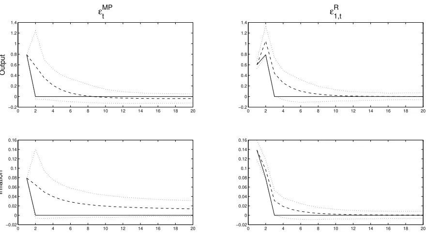
Figure 1: Impulse Responses of Endogenous Variables to Unanticipated and Forward Guidance Shocks. Solid Line: Rational Expectations; Dashed Line: CGL; Dotted Lines: 95% Confidence Bands.

distribution centered around its rational expectations counterparts. Thus, the initial impact under

adaptive learning could be greater or less than the initial impact under rational expectations.

After Impact–Figures 1 and 2 also display the impulse responses after the forward guidance

announcement is known to agents. From the household’s perspective, they must optimally allocate

consumption across time based on their expectations of future variables. Since they know that

the interest rate will decrease in the future, a household changes its optimal consumption across

time and increases current consumption. In addition, firms know they may not be able to change

their price in the future regardless of the state of the economy. Thus, they take into account

expectations of future variables as seen in equation (18). When the central bank announces that

the interest rate will increase in the future, a firm knows that the future output gap and inflation

will be affected, and thus, this action affects current pricing decisions. Furthermore, there exists

a larger and more delayed effect on the economy under a forward guidance shock than under an

unanticipated monetary policy shock. This result is similar to Milani and Treadwell (2012).

The impulse responses show that adaptive learning agents fail to understand the precise effect

an announcement to lower the future interest rate will have on the economy. Adaptive learning

0 2 4 6 8 10 12 14 16 18 20 −0.5

0 0.5 1 1.5 2

Output

ε_8,tR

0 2 4 6 8 10 12 14 16 18 20 −1

−0.5 0 0.5 1 1.5 2

ε_12,tR

0 2 4 6 8 10 12 14 16 18 20 −0.05

0 0.05 0.1 0.15 0.2 0.25 0.3 0.35

Inflation

0 2 4 6 8 10 12 14 16 18 20 −0.05

0 0.05 0.1 0.15 0.2 0.25 0.3 0.35 0.4

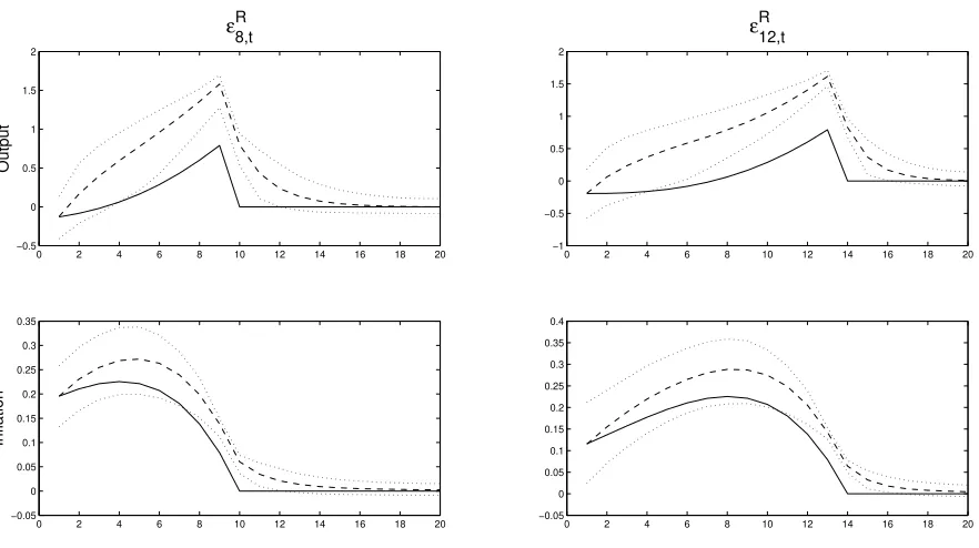
Figure 2: Impulse Responses of Endogenous Variables to Forward Guidance Shocks. Solid Line: Rational Expectations; Dashed Line: CGL; Dotted Lines: 95% Confidence Bands.

they do not understand the precise effect this shock will have on the economy, adaptive learning

agents are continually readjusting their forecasts each period causing the impulse responses to

ex-hibit more persistence than under rational expectations. In addition, when the forward guidance

shock has been realized upon the economy, there exists a greater substitution effect under adaptive

learning than rational expectations. Adaptive learning agents substitute into more consumption

than rational expectations agents. The former agents overshoot their rational expectations

coun-terparts. This conclusion occurs because rational expectations agents precisely know how the

an-ticipated changes in monetary policy will affect the endogenous variables at later dates. However,

adaptive learning agents imprecisely understand how a commitment to lower the future interest

rate will have on the economy since they do not know the true model of the economy.

After Shock Realized–The impulse response graphs of rational expectations and adaptive

learning do not follow the same path after the shock is realized upon the economy. The impulse

responses with rational expectations agents converge quicker to zero percentage deviation from the

unshocked series. Rational expectations agents understand that the shock will not occur in the

future and they quickly adjust their expectations. However, the impulse responses under adaptive

learning exhibit more persistence than the impulse responses under rational expectations. This

driven by adjustments in the beliefs of the agents. Adaptive learning agents revise their estimates

of the parameters of the economy each period, while rational expectations agents fully understand

the model’s parameters. The impulse responses of a conventional monetary policy shock shown in

the first column of Figure 1 also display the same difference in persistence.

The results coincide with the literature on adaptive learning. The outcomes match Eggertsson

(2008) who found that temporary policy shifts do not have as large of an effect on the economy as

permanent policy shifts under the assumption of rational expectations. The persistence results also

coincide with Milani (2007) who found that a DSGE model with constant-gain learning generates

persistence in the macroeconomic variables.

To summarize, the message from this section is that adaptive learning agents fail to

under-stand the precise effect a forward guidance announcement has on the economy. When the forward

guidance shock is known to agents, the output gap and inflation rate under adaptive learning

proceed in a different path than under rational expectations. After the shock has been realized,

rational expectations agents quickly adjust their expectations to the knowledge that the shock

is gone, while adaptive learning agents’ beliefs are more persistent. These results are attributed

to rational expectations agents precisely understanding the effects forward guidance has on the

economy, while the beliefs of adaptive learning agents slowly adjust.

4.2.2 Policy Exercise

The results displayed by the impulse response functions showed that adaptive learning agents failed

to understand the precise effects forward guidance has on the economy. This current section shows

this conclusion through a different scenario. Specifically, the central bank would like to keep the

interest rate fixed at a certain level ¯i forL+ 1 periods. The experiment is described next and is

motivated by the policy exercise described in Del Negro et al. (2012).

Suppose at the beginning of period T, the central bank implements forward guidance such

that the interest rate will be fixed at ¯i = 0 in period T and L periods into the future. This

announcement corresponds to an unanticipated shock in period T and news about the future

interest rate 1,2, . . . , L periods into the future. In this scenario, the monetary policymaker’s job

is to choose εM P

T and ηT = [εR1,T, . . . , εRL,T] ′

such that the interest rate in periods T to T +L

equals ¯i. The central bank also believes that agents hold rational expectations, which is a common

assumption in macroeconomic literature. To show that adaptive learning agents respond differently

to the same forward guidance information, the adaptive learning agents are given the same guidance

periodT.20 _{The model is then simulated from T to the end of the forward guidance horizonT+L.}

The process is then repeated 5,000 times and the mean across the 5,000 simulations is calculated.

This policy exercise also assumes that the central bank is committed to its goal of ¯i every

period during the forward guidance horizon. Rational expectations agents precisely understand the

central bank’s guidance, and thus, the interest rate each period implied by rational expectations

equals ¯i. Since the adaptive learning process is different than rational expectations, the same

forward guidance will not give a model implied ¯iduring the forward guidance horizon. To model a

commitment to ¯i= 0, the central bank choosesεM P

t each period over the forward guidance horizon

to ensure the interest rate equals ¯i.21

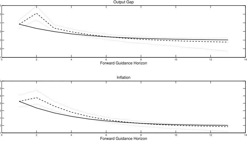
Figure 3 compares the dynamics under rational expectations and adaptive learning for the

output gap and inflation. The values of the output gap and inflation during the forward guidance

horizon are averaged across simulations. The solid line represents rational expectations while the

dashed line line displays the adaptive learning path. Under both expectations assumptions, forward

guidance has an obvious stimulative effect on impact. Since interest rates are lowered, the output

gap and inflation increase. As time elapses and the forward guidance horizon draws to an end,

the stimulative effects of this central bank policy fade away. In addition, since adaptive learning

agents’ beliefs are distributed around its rational expectations counterparts, the initial effect is

approximately the same under both series. However, the effect under adaptive learning could vary

from rational expectations depending on adaptive learning agents’ beliefs used at timeT to forecast

future variables.

Figure 3 also shows that adaptive learning agents fail to understand how the same forward

guidance commitments made under rational expectations will impact the economy under learning.

This results in larger variation in both the output gap and inflation and a slower speed back

to long-run equilibrium under adaptive learning than under rational expectations. The adaptive

learning agents observe the unanticipated lowering of the interest rate in period T. In the next

period, they adjust their expectations of the output gap and inflation upwards due to this previous

information. The adaptive learning path then continues at a downward path quicker than under

rational expectations. Furthermore, the effect from central bank forward guidance results in more

pessimism under adaptive learning than under rational expectations at longer horizons. By having

only partial information about the true model of the economy, adaptive learning agents fail to

foresee the precise positive impact the forward guidance information has on the dynamics of the

20

T is chosen to be a large number so that the adaptive learning coefficients converge to its stationary distribution.

21

0 2 4 6 8 10 12 14 −1

−0.5 0 0.5 1 1.5 2

Output Gap

Forward Guidance Horizon

0 2 4 6 8 10 12 14

−0.1 0 0.1 0.2 0.3 0.4 0.5 0.6

Inflation

Forward Guidance Horizon

Figure 3: Dynamics of the Output Gap and Inflation in Response to Forward Guidance. Solid Line: Rational Expectations; Dashed Line: CGL; Dotted Lines: 95% Confidence Bands.

output gap and inflation. Thus, this aspect leads to a period of undershooting on the part of

adaptive learning agents. The output gap and inflation under adaptive learning fall short of the

paths of rational expectations at longer horizons. Rational expectations agents, however, precisely

understand the effects of forward guidance on the output gap and inflation. They understand the

stimulative effect forward guidance has on the economy, and thus, the output gap and inflation is

higher than under adaptive learning over this latter period.

The source of this difference between the two paths regards the assumptions made under

rational expectations and adaptive learning. The rational expectations agents know the true model

and aggregate probabilities. They can infer the precise effect forward guidance has on the economy.

However, the expectations of adaptive learning agents do not respond in the same way. Adaptive

learning agents do not know the true model of the economy, and thus, cannot infer the proper

aggregate probabilities and expectations. Even though they know the changes in the future path

of interest rates implemented by the central bank, adaptive learning agents imprecisely understand

how that guidance impacts the economy. Since they readjust their forecasts each period, adaptive

learning agents overshoot and undershoot the paths implied by rational expectations. Moreover,

this result shows a consequence of the decision of monetary policymakers. If the central bank

assumes agents have rational expectations, which is standard in the macroeconomic literature, the

displays a different path than what would occur under rational expectations.

4.3 Economic Crisis

In response to the 2007-2009 Great Recession, forward guidance was implemented by central banks

around the world. With that event in mind, this section builds upon the previous subsection’s

exercise by considering forward guidance during an economic recession. The economy is assumed

to start in periodT, that is, after a period of economic stability (corresponding to say the period

before the recent Great Recession).22 The model is then simulated from T to the end of the

forward guidance horizon T +L. As in the previous subsection, the central bank implements

forward guidance by choosing the unanticipated monetary policy and anticipated forward guidance

shocks such that the nominal interest rate equals zero from periodsT toT+L. To capture features

from the recent Great Recession, a large negative demand shock impacts the economy in periodT,

and causes a recession. A sequence of five more negative demand shocks follows so that the recession

lasts six periods.23 _{In the following periods, the shocks are drawn from a normal distribution. Thus,}

the forward guidance horizon spans a recession and normal times. The process is then repeated

5,000 times and the mean across the 5,000 simulations is calculated.

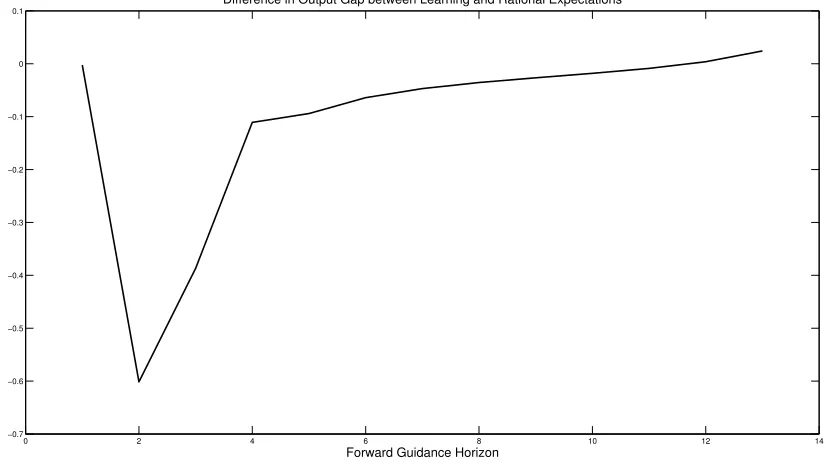
Figure 4 displays the macroeconomic effects of forward guidance during an economic recession.

The graph shows the value of the output gap under adaptive learning minus the value of the output

gap under rational expectations.24 Under both expectations formation assumptions, the negative

demand shocks cause the output gap to drop below its steady state value. However, the positive

effects of forward guidance are overstated under the assumption of rational expectations relative

to adaptive learning. Throughout the forward guidance horizon, the value of the output gap under

rational expectations is higher than under adaptive learning. The former agents know the economy

is in a recession and precisely understand how forward guidance will alleviate the economy as

their expectations are based on the true model of the economy. However, adaptive learning agents

observe the economic downturn, but fail to completely understand the positive effects of forward

guidance. They must estimate the effects of forward guidance on the economy as their forecasts

are based on an econometric model. Thus, adaptive learning agents are slower to understand how

forward guidance will alleviate the downturn in the economy.

Additional intuition for the results of this section is displayed in Figure 5, which shows the

22

This strategy also ensures the adaptive learning coefficients converge to its stationary distribution.

23

This length is based on the duration of the Great Recession as defined by the National Bureau of Economic Research.

24

0 2 4 6 8 10 12 14 −0.7

−0.6 −0.5 −0.4 −0.3 −0.2 −0.1 0 0.1

Difference in Output Gap between Learning and Rational Expectations

Forward Guidance Horizon

Figure 4: Macroeconomic Effects of Forward Guidance during an Economic Crisis

values of adaptive learning minus rational expectations of the discounted long-run expectations of

the output gap, inflation and the interest rate across the forward guidance horizon. The adaptive

learning agents are more pessimistic about the future output gap and inflation as their long-run

expectations are lower than under rational expectations. The former are overestimating the

ram-ifications of the downturn in the economy and their estimates of the effects of forward guidance

are not strong enough to overcome this negative reaction. However, rational expectations agents

understand the effects of the economic downturn and how forward guidance will precisely alleviate

the economy.

The results in Figure 5 also relate to the empirical findings of Del Negro et al. (2012). Their

model, which was solved under the assumption of rational expectations, produced an exceedingly

large reaction of the macroeconomic variables to forward guidance statements. Del Negro et al.

(2012) argued that the source of the excessive responses was an unusually large drop of the

long-run interest rate to forward guidance statements relative to the data. In this current paper, the

bottom panel of Figure 5 shows a comparable result: the long-run expectation of the interest rate

is lower under rational expectations than adaptive learning. This produces larger responses of

long-run expectations of the output gap and inflation, and consequently, the current output gap

and inflation under rational expectations than adaptive learning. Thus, this result suggests two

additional takeaways. A forward guidance model better matches the data under the assumption

0 2 4 6 8 10 12 14 −0.6

−0.4 −0.2 0 0.2

Difference in Long Run Expectations of the Output Gap

0 2 4 6 8 10 12 14

−0.06 −0.04 −0.02 0

0.02 Difference in Long Run Expectations of Inflation

0 2 4 6 8 10 12 14

−0.2 0 0.2 0.4 0.6

Forward Guidance Horizon

Difference in Long Run Expectations of the Interest Rate

Figure 5: Difference between Adaptive Learning and Rational Expectations Infinite Horizon Expectations of the Macroeconomic Variables. A positive value indicates the value under adaptive learning is higher than under rational expectations. A negative value indicates the variable’s value under adaptive learning is lower than under rational expectations.

macroeconomic variables to forward guidance found in Del Negro et al. (2012) could be due to the

way in which expectations are modeled.

Overall, the results suggest a main finding for policymakers. If monetary policy is based

on a model with rational expectations, which is the standard assumption in the macroeconomic

literature, the results may be misleading. This section shows that the assumption of rational

expec-tations overstates the effects of forward guidance relative to adaptive learning during an economic

recession. The adaptive learning results also match the data better than rational expectations.

5

Extensions

5.1 Alternative Parameterization

The results of this paper are investigated under different values ofσ, the intertemporal elasticity of

substitution parameter. σmeasures the effect current and future real interest rates have on current

consumption and output. This parameter is important since forward guidance involves statements

0 2 4 6 8 10 12 14 16 18 20 −0.5 0 0.5 1 1.5 2 2.5 X ε 8,t R

Impulse Response Function Horizon

0 2 4 6 8 10 12 14 16 18 20

−0.5 0 0.5 1 1.5 2 2.5 ε 12,t R

Impulse Response Function Horizon

0 2 4 6 8 10 12 14 16 18 20

−0.05 0 0.05 0.1 0.15 0.2 0.25 0.3 0.35 π

Impulse Response Function Horizon

0 2 4 6 8 10 12 14 16 18 20

−0.05 0 0.05 0.1 0.15 0.2 0.25 0.3 0.35

Impulse Response Function Horizon

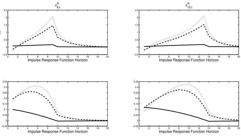
Figure 6: Impulse Response Functions to Forward Guidance Shocks Under Different Values of σ. Solid Line: σ= 0.15; Dashed Line: σ= 1; Dotted Line: σ= 1.5

paper investigates the outcomes of the model when σ = 0.15, σ= 1, and σ= 1.5.25 These results

are displayed via adaptive learning impulse responses of the output gap and inflation to negative

one unit forward guidance shocks similar to Section 4.2.1.

The results displayed in Figure 6 show that higher values of σ produce greater forward

guidance effects than lower values of σ. As σ increases, the output gap responds more to current

and future real interest rates. Thus, since forward guidance involves information about future

nominal interest rates, demand responds more to news that the interest rate will decrease in the

future. Asσdecreases, the output gap does not respond as much to changes in current and expected

future interest rates. Therefore, the impact of policy shocks on the economy is less pronounced.

Overall, the impulse responses of the output gap and inflation are not as responsive to forward

guidance news in comparison to results under a higher value of σ.

5.2 Alternative Constant Gains

In this section, a robustness exercise is simulated to examine the effects of forward guidance

pol-icy when adaptive learning agents vary the degree in which they discount previous observations.

Specifically, higher and lower values of the gain parameter, ¯τ, are used. In addition to ¯τ = 0.02,

the other constant gains assumed are ¯τ = 0.01 and ¯τ = 0.05.

25

0 2 4 6 8 10 12 14 16 18 20 −0.2 0 0.2 0.4 0.6 0.8 1 1.2 1.4 1.6 X ε 8,t R

Impulse Response Function Horizon

0 2 4 6 8 10 12 14 16 18 20 −0.5 0 0.5 1 1.5 2 ε 12,t R

Impulse Response Function Horizon

0 2 4 6 8 10 12 14 16 18 20 −0.05 0 0.05 0.1 0.15 0.2 0.25 0.3 π

Impulse Response Function Horizon

0 2 4 6 8 10 12 14 16 18 20 −0.05 0 0.05 0.1 0.15 0.2 0.25 0.3

Impulse Response Function Horizon

Figure 7: Impulse Response Functions to Forward Guidance Shocks under Different Values of ¯τ. Solid Line: CGL with ¯τ = 0.01; Dashed Line: CGL with ¯τ = 0.02; Dotted Line: CGL with ¯

τ = 0.05.

The results in Figure 7 show that the responses of the macroeconomic variables to forward

guidance under adaptive learning depend on the value of ¯τ. From the time of the forward guidance

announcement to when the shock is realized, agents with higher constant gains seem to misvalue

more the effects of forward guidance than agents with lower constant gains. Under higher values of

¯

τ, agents place more weight on new information, and thus, exhibit a stronger reaction to forward

guidance news. Each period’s estimates and beliefs should vary more from the previous period’s

estimates. However, under lower values of ¯τ, agents do not misvalue the effects of forward guidance

as much as under higher values of ¯τ. They do not exhibit as strong of a reaction to forward guidance

news as agents with a higher value of ¯τ. Moreover, after the shock is realized on the economy, agents

with a higher ¯τ are quicker to realize the shock is not present as they weight previous observations

more than agents with a lower ¯τ. Thus, the impulse responses under higher values of ¯τ are quicker

to return to zero percentage deviation from the unshocked series than under lower values of ¯τ.

6

Conclusion

In order to combat the effects of the 2007-2009 global financial crisis, central banks around the

world have instituted forward guidance. Because the effectiveness of forward guidance hinges on how