Automatic streamlining for constrained optimisation

Patrick Spracklen, Nguyen Dang, ¨Ozg¨ur Akg¨un, Ian Miguel

School of Computer Science, University of St Andrews, St Andrews, UK

{jlps, nttd, ozgur.akgun, ijm}@st-andrews.ac.uk

Abstract. Augmenting a base constraint model with additional constraints can

strengthen the inferences made by a solver and therefore reduce search effort. We focus on the automatic addition ofstreamlinerconstraints, which trade complete-ness for potentially very significant reduction in search. Recently an automated approach has been proposed, which produces streamliners via a set of streamliner generation rules. This existing automated approach to streamliner generation has two key limitations. First, it outputs a single streamlined model. Second, the ap-proach is limited to satisfaction problems. We remove both limitations by provid-ing a method to produce automatically aportfolioof streamliners, each represent-ing a different balance between three criteria: how aggressively the search space is reduced, the proportion of training instances for which the streamliner admitted at least one solution, and the average reduction in quality of the objective value versus the unstreamlined model. In support of our new method, we present an automated approach to training and test instance generation, and provide several approaches to the selection and application of the streamliners from the portfolio. Empirical results demonstrate drastic improvements both to the time required to find good solutions early and to prove optimality on three problem classes.

Keywords: Constraint Programming·Streamliners

1

Introduction

An initial constraint model can be augmented through additional constraints. If well chosen, these constraints strengthen the inferences the solver can make and therefore reduce search.Impliedconstraints are inferred directly from the initial model and there-fore do not alter the set of solutions to the model. Manual [15,16] and automated [7,9,17] approaches to generating implied constraints have been successful.

In contrast,streamlinerconstraints [20] (our focus herein) are not inferred from the initial model and often radically alter the set of solutions to the model in an attempt to focus effort on a highly restricted but promising portion of the search space. Streamlin-ers trade the completeness offered by implied constraints for potentially much greater search reduction. They were originally derived manually by examining solutions of small instances of a problem class for patterns, which were used as the basis for stream-liners [20,22,23,24]. For example Gomes and Sellmann added a streamliner requiring a latin square structure when searching for diagonally ordered magic squares [20].

under consideration, streamliner candidates are evaluated automatically and the most promising ones are used to solve more difficult instances from the same problem class. The existing automated approach to streamliner generation has two key limitations. First, it outputs a single streamlined model. If on a test instance this streamliner excludes all solutions the only remedy is to revert to the initial model. Second, the approach is limited to satisfaction problems. We remove both limitations by providing a method to produce automatically aportfolioof streamliners, each representing a different balance between three criteria: how aggressively the search space is reduced, the proportion of training instances for which the streamliner admitted at least one solution, and the average reduction in quality of the objective value versus an unstreamlined model.

In support of our new method, we present an automated approach to training and test instance generation, and provide several approaches to the selection and application of the streamliners from the portfolio. The result is the first automatic method to produce streamliners for optimisation problems and to offer alternatives if the most preferred streamliner is unsuccessful.

2

Candidate Streamliner Generation

As in [32], our approach proceeds from a specification of a problem class in the ab-stract constraint specification language ESSENCE[14], such as the SONET example in Figure 1. An ESSENCEspecification comprises the problem class parameters (given); the combinatorial objects to be found (find); the constraints the objects must satisfy (such that); identifiers declared (letting); and an optional objective function (min/maximising). The key feature of the language is support for abstract deci-sion variables, such as multiset, relation and function, as well asnestedtypes, such as the multiset of sets in Figure 1.

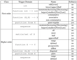
The highly structured description of a problem an ESSENCEspecification provides is better suited to streamliner generation than a lower level representation, such as a constraint modelling language like MiniZinc [27]. This is because nested types like multiset of sets must be represented as a constrained collection of more primitive vari-ables, obscuring the structure that is useful to drive streamliner generation. We employ the same set of streamliner generation rules as [32], summarised in Table 1. High-order rules take another rule as an argument and lift its operation onto a decision variable with a nested domain such as the complex multi-set structure present in SONET. This allows for the generation of a rule such as enforcing that approximately half (with soft-ness parameter) of the sets in the multiset only contain even numbers. Imposing extra structure in this manner can reduce search very considerably. Table 2 presents candi-date streamliners automatically generated for the problem classes considered herein. Although rich, the set of ESSENCEtype constructors is not exhaustive. Graph types, for example, are a work in progress [10]. At present, therefore, we might specify such a problem in terms of a set of pairs. The streamliner generator constraints would produce candidate streamliners based on this representation.

solver-1 $ SONET

2 given nnodes, nrings, capacity : int(1..) 3 letting Nodes be domain int(1..nnodes) 4 given demand : set of set (size 2) of Nodes 5

6 find network : mset (size nrings) of

7 set (maxSize capacity) of Nodes

8 minimising sum ring in network . |ring|, 9 such that forAll pair in demand .

10 exists ring in network . pair subsetEq ring 11

12 $ Minimum Energy Broadcast

13 letting dNodes be domain int(1..n_nodes) 14 letting dDepths be domain int(1..n_nodes) 15 find parents: function (total)

16 dNodes --> dNodes,

17 depths : function (total)

18 dNodes --> dDepths

19

20 $ Progressive Party

21 letting Boat be domain int(1..n_boats) 22 find hosts: set (minSize 1) of Boat, 23 sched: set (size n_periods) of

24 function (total) Boat --> Boat

Fig. 1: ESSENCEspecifications for the three problem classes considered herein. Synchronous Optical Networking (SONET) [28] is given in full. For brevity, only the parameters and decision variable declarations (from which streamliners are generated) are shown for the Progressive Party Problem [33] and the Minimum Energy Broadcast Problem [6]

independent constraint modelling language ESSENCEPRIME, which SAVILEROW[29] translates into input suitable for the constraint solver MINION[19].

3

Searching for a Streamliner Portfolio

Candidate streamliners are often most effectively used in combination [20]. In an at-tempt to find a single “best” streamlined model, Spracklen et al. described a Monte Carlo Tree Search [5] (MCTS)-based algorithm to search the lattice of models where the root is the original ESSENCEspecification and an edge represents the addition of a streamliner to the combination associated with the parent node.

satisfaction problems by bounding the objective and searching for a satisfying solution. This is a serious limitation since a candidate streamlined model may find a solution quickly, but of poor quality, and may exclude the set of optimal solutions entirely.

Class Trigger Domain Name Softness

First-order

int odd{even} no

lower{upper}Half no

function int --> intmonotonicIncreasing{Decreasing} no largest{smallest}First{Last} no

function (X,X) --> X

commutative no

associative no

non-commutative no

partition from X quasi-regular yes

sequence montonicIncreasing{Decreasing} no largest{smallest}First{Last} no

Higher-order

matrix/set of X

all no

most yes

half no

approxHalf yes

function X --> Y

range no

defined no

pre{post}fix yes

allBut yes

function (X,X) --> Y diagonal no

partition from X parts no

sequence range no

defined no

Table 1: The rules used to generate conjectures. Rows with a softness parameter specify a family of rules each member of which is defined by an integer parameter.

Problem Streamliner Description

Id

Sonet 6 Exactly half the nodes installed on each ring are odd.

13 Approx. half the nodes installed on each ring are odd.

15 Approx. half the nodes on each ring are from the lower half of the Nodes domain. 67 The objective variable is constrained to the lower half of its domain MEB 18 Approx. half of the entries in the range of the parents function must be even

41 The range of the depths function contains all odd entries

PPP 7 For half of the hosts the boats must be in the lower half of the Boats domain

14 For approx. half of the hosts the Boats must be odd

To address these problems we adopt a multi-objective optimisation approach, where each pointxin the search spaceX is associated with ad-dimensional (dis the number of objectives) reward vectorrxinRd. Our three objectives allow us explicitly to bal-ance considerations of solution quality against how aggressively the streamlined model reduces search:

1. Applicability. The proportion of training instances for which the streamlined model admits a solution.

2. Search Reduction. The mean reduction in time to prove optimality in comparison with an unstreamlined model.

3. Optimality Gap. The mean percentage difference between the optimal value found by the streamlined model and the true optimal value under the unstreamlined model. All objectives are transformed such that they can be maximized. With these three objectives for each streamliner combination we define a partial ordering on Rd _and so on X using the Pareto dominance test. Given x, x0 ∈ X with vectorial rewards rx = (r1, . . . , rd)andrx0 = (r10, . . . , rd0)rx dominates rx0 iffri is greater than or equal tori0fori= 1. . . d.

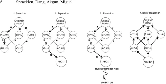
To search the lattice structure for a portfolio of Pareto optimal streamlined models we have adapted thedominance-based multi-objective MCTS (MOMCTS-DOM) algo-rithm [34]. This has four phases, as summarised below and in Figure 2:

1. Selection: Starting at the root node, the Upper Confidence Bound applied to Trees (UCT) [5] policy is applied to traverse the explored part of the lattice until an un-expanded node is reached.

2. Expansion: Uniformly select and expand an admissible child

3. Simulation: The collection of streamliners associated with the expanded node are evaluated. The vectorial reward (Applicablity, Search Reduction, Optimality Gap) across the set of training instances is calculated and returned.

4. BackPropagation: The current portfolio; which contains the set of non dominated streamliner combinations found up to this point during search; is used to compute the Pareto dominance. The reward values of the Pareto dominance test are non sta-tionary since they depend on the portfolio, which evolves during search. Hence, we use the cumulative discounted dominance (CDD) [34] reward mechanism during reward update. If the current vectorial reward is not dominated by any streamliner combination in the portfolio then the evaluated streamliner combination is added to the portfolio and a CDD reward of 1 is given, otherwise 0. Dominated stream-liner combinations are removed from the portfolio. The result of the evaluation is propagated back up through all paths in the lattice to update CDD reward values, as shown in the figure.

4

Generating Diverse Training Instances

Fig. 2: MOMCTS-DOM operating on the streamliner lattice. A, B and C refer to single candidate streamliners generated from the original ESSENCEspecification. As MOMCTS-DOM descends down through the lattice the streamliners are combined through the conjunction of the individual streamliners (AB, ABC). The nodes are labelled withCDD reward value/times visited.

the problem class. To ensure diversity, we employ an automated approach combining a per-class parameter generator and an algorithm configuration tool, described below.

For each problem class we wrote a simple instance generator that accepts a param-eter setting and a random seed, and outputs a problem instance. At the moment the instance generator has to be manually created, and is the only part of the whole sys-tem that is not automated. However, this issue has been tackled in a recent work [2] within the same pipeline, which can be integrated into our system in the future. To keep the computational cost manageable, we require a set of relatively easy (but not trivial) instances for the training phase, which we define as solvable by MINION[19] on an unstreamlined model within a time limit of[10,300]seconds.

To find instances satisfying our criteria, the automatic algorithm configuration tool irace [25] is used. Parameters of each generator are tuned by irace with a performance measure guiding it towards regions of satisfiable instances within the required range of solving time. As the tuning procedure usually converges at certain regions of the search, multiple tunings with two settings of irace (the default and another that allows more exploration) are performed per problem class to obtain more diverse sets of instances.

There is an inherent tradeoff with the number of training instances used during search. If too few instances are used it diminishes the ability of the generated portfolios to generalise across the problem class, whereas a larger set reduces the iteration speed of MOMCTS to the point where it is ineffective in searching the streamliner lattice. Taking these considerations into account, for the experiments in this paper we have set the number of training instances to 50.

Problem Total Number Number Of Of Instances Clusters

SONET 517 3

MEB 989 8

PPP 1264 8

Table 3: Instance Generation and Clustering. 50 training instances are selected from among the generated clusters.

features are normalised according to the z-score standardisation. GMeans clustering is used on the generated features to detect the number of instance clusters (see column 3 of Table 3). To build the training set instances are randomly selected from each cluster, with the number of instances taken from each weighted according to the relative size of each cluster.

The time limit for training instances, and the size of the training set are both param-eters to our method, which will be investigated in future work.

5

Pruning the Streamliner Portfolio

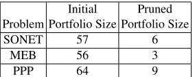
As the number of objectives increases so, typically, does the size of the Pareto front, and hence the size of the generated streamliner portfolio. This is demonstrated in Table 4, which, in column 2, records the size of the streamliner portfolios generated through MOMCTS for our three problem classes. A large portfolio is cumbersome when consid-ering streamliner selection and scheduling. We observed, however, that the streamlined models were not distributed evenly across the Pareto front. Therefore, GMeans cluster-ing is used to identify the number of clusters present in the portfolio and a point from each cluster is then selected to form a representative subset of the full portfolio (see column 3 of Table 4).

Initial Pruned

Problem Portfolio Size Portfolio Size

SONET 57 6

MEB 56 3

PPP 64 9

Table 4: We prune an initially generated streamliner portfolio through GMeans clustering and select a representative point from each cluster.

6

Selecting from the Streamliner Portfolio

Algorithm 1Lexicographic Streamliner Selection

procedureSELECTION(Portfolio P, Ordering,T imetotal, Instance)

P←sort(P, by = Ordering) T imeT aken←0

while T imeT aken≤T imeT otaldo

Streamliner←P.next()

Stats←Apply(Streamliner, Instance) ifStats→sat()then

setBound(Instance, Stats.bound) .Set new bound on the instance end if

T imeT aken+ =Stats.time end while

end procedure

which streamlined models from the portfolio should be used, in what order, and accord-ing to what schedule. We consider both static lexicographic selection methods, which establish a priority order over our three objectives of Applicability, Search Reduction and Optimality Gap, and a dynamic method, which adjusts the selection based on the performance on the instance thus far.

6.1 Lexicographic Selection Methods

It is possible to order the streamlined models in a portfolio lexicographically by, for example, prioritising Applicability, then Search Reduction, and finally the Optimality Gap. Given three objectives, there are six such orderings to consider. Through prelimi-nary testing it became apparent that only two of these orderings are effective, where the Applicability objective is prioritised. The other orderings trade Applicability for either Search Reduction or a better Optimality Gap. On more difficult test instances, signifi-cant search effort can be required to prove that an aggressive streamliner has rendered an instance unsatisfiable, which can lead to poor overall performance. Thus two lexi-cographic selection methods are used herein:{Applicability First, Optimality Second, Reduction Third}and{Applicability First, Reduction Second, Optimality Third}.

The selection process involves traversing the portfolio (using the defined ordering) for a given time period and applying each streamliner in turn to the given instance as shown in Algorithm 1. The schedule is static in that it only moves to the next stream-lined model when the search space of the current one is exhausted. A key parameter isT imetotal, which specifies the total budget in seconds for traversing the streamliner portfolio. In Section 8 for each selection method four different settings for this param-eter are experimented with to explore its effect on overall performance.

6.2 UCB Streamliner Selection

Algorithm 2UCBSelection

procedureSELECTION(Portfolio, Ordering,T imetotal, Instance)

T imetaken←0 UCBTimeLimit←1 NumberOfIterations←0

Map .Mapping from Streamliner to Process

whileT imetaken≤T imetotaldo

Streamliner←UCTSelection(Portfolio) if Map[Streamliner].restartthen

Process←remodel(instance, streamliner) .Remodel with the new bound Map[Streamliner].process←Process

Stats←run(Process, UCBTimeLimit) else

Process←Map[Streamliner].process

Stats←run(Process, UCBTimeLimit) .Continue running existing process end if

Map[Streamliner].visits += 1 NumberOfIterations += 1 ifStats→sat()then

Map[Streamliner].reward += 1

setBound(Instance, Stats.bound) .Set new bound on the instance

forS←M apdo

ifS != Streamlinerthen

Map[S].restart = True .New Bound was found; restart all other processes end if

end for end if

T imetaken+ =Stats.time end while

end procedure

For each streamlinerkwe record the average rewardxk _{and the number of times} khas been tried in the selection (nj) out of a total ofniterations. On each iteration a streamliner is chosen that maximizesxk+p2 log(n)/nj. The reward distributions for an individual streamliner are not fixed, so this is not a Stationary Multi-Armed Bandit problem. However, if a streamliner performs well, we expect it will continue performing well during search even if there is a slight variation in the mean reward. We have found that using UCB1 gives good results. Future work could investigate the use of Upper Confidence Bound policies for non-stationary bandit problems, such as the family of Exp3 algorithms [21,26].

When traversing the portfolio UCB performs incremental evaluation, it runs a stream-liner for a set time, observes the results, and potentially moves on before the correspond-ing search space has been exhausted. When the streamliner is pre-empted it is necessary to pause the search in order to avoid repeating work if it is rescheduled at a later point. The only exception to this is whenever a new bound on the objective is discovered all of the streamliners from the portfolio, aside from the current streamliner, are restarted and remodeled with the new bound. There are two main benefits to doing this. Firstly, by restarting the streamliner has the newly constrained bound at the top of the search tree which allows it to make more informed decisions higher up without descending into unsatisfactory subtrees. Secondly, by remodeling it takes advantage of the toolchain (CONJUREand SAVILEROW) which may be able to reformulate the model based upon this new information and produce reductions at the solver level. Algorithm 2 shows the UCBSelection process in detail.

7

Experimental Setting

We evaluate our automated streamlining approach on the three problem classes in Fig-ure 1. We selected these problems to give good coverage of the abstract domains avail-able in ESSENCE, such as set, multi-set and function. Furthermore, SONET and Pro-gressive Party have nested domains: multi-set of set and set of function respectively.

Our hypothesis is that a streamliner portfolio, generated automatically on a set of automatically generated training instances from a given problem class, can be employed to solve more difficult test instances to deliver substantial performance improvements relative to an unstreamlined model. Training instances were generated as per Section 2, with a time limit of[10,300]seconds. Test instances are generated using the same instance generator and the tuning tool irace but with a time limit of(300,3600]seconds. 50 instances are selected randomly to form the test set.

All experiments were run on a cluster of 280 nodes, each with two 2.1 GHz, 18-core Intel Xeon E5-2695 processors. MOMCTS was run on a single core with a budget of 4 CPU days for each problem class. Results on 50 test instances under the unstream-lined and streamunstream-lined models are reported, where every test instance was run with three random seeds.

Source code, instance generators, datasets and detailed results are available at https: //github.com/stacs-cp/CP2019-Streamlining.

8

Results

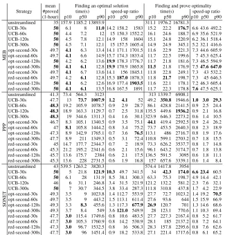
Table 5 summarises results on 50 test instances (3 runs/instance) for each of our three problem classes. We evaluate four different approaches: an unstreamlined model, and streamliner portfolios with UCB selection, lexicographic ordering{Applicability First, Optimality Second, Reduction Third}(denotedopt-second), and lexicographic ordering {Applicability First, Reduction Second, Optimality Third} (denotedred-second). For each streamliner selection method, a parameter is the amount of time allocated to the streamliner portfolio before handing over to the unstreamlined model to prove optimal-ity. Four different values for this time budget were tested: 30, 60, 120 and 300 seconds. Results in Table 5 are strongly positive. They show that all the streamliner portfo-lio approaches can not only find an optimal solution and prove optimality on more test instances than the unstreamlined model, but also vastly reduce the amount of time re-quired for both tasks. In general, the UCB-30s variant has the best overall performance across the three problem classes, and provides consistently robust improvement over the unstreamlined model.

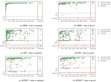
Figure 3 presents more details of how the streamliner approaches improve on the unstreamlined models on an instance basis. In these plots, we use the time-reduction ratio, a “normalised” version of the speed-up values reported in Table 5 for presentation: as the speed-up values can be arbitrarily large, many data points in the speed-up plots can appear in a very small range, making them difficult to distinguish. The reduction ratio, which is calculated as1−1/speed-up, is limited to at most one and can be easily scaled. For brevity, we only show in Figure 3 results of the streamliner variants with the time limit of 30 seconds. Each data point corresponds to a pair of instances and random seeds. The plots show that the solving time of the test instances are well distributed across the x-axis, which is a good indication for the diversity of the test instance set. There are several cases where the unstreamlined model cannot find or prove optimality within the time budget and the streamliner can, which are represented by the data points on the rightmost side after the vertical red lines.

mean Finding an optimal solution Finding and prove optimality Strategy #proved time(s) speed-up ratio time(s) speed-up ratio

(1-hour) p10 p50 p90 p10 p50 p90 p10 p50 p90 p10 p50 p90

MEB

unstreamlined 35 157.9 1185.2 13893.9 311.1 1976.2 16781.3

UCB-30s 50 6.1 8 11.014.2 158.2 1583 15.2 22.2 176.7 6.6 43.6 492.2 UCB-60s 50 4.4 7.2 12 15 150.3 1552.2 16.1 24.6 188.7 6.9 35.6 521.9 UCB-120s 50 4.5 7.8 12.1 14.9 158 1604 15.1 24.8 220.9 6.2 36.1 518.4 UCB-300s 50 4.5 7.1 12.1 15 157.5 1605.4 14.9 24.9 345.1 5.2 32.1 416.6 opt-second-30s 49.7 4.1 6.3 13.4 14.1 171.1 1701.5 11.6 22.9 221.3 7.3 44.6 605.9 opt-second-60s 49.7 4.1 6.6 14.9 15.7 174.3 1833.4 11.7 22.5 199.6 7 45.3 625.4 opt-second-120s 50 4.2 6.2 13.619.9178.3 1776.7 11.7 21.8 181.6 7.3 46.5 594.9 opt-second-300s 50 4.1 6.1 12.819.9170.9 1865.8 11.5 21.8 176.9 7.547.6 647.0 red-second-30s 49.7 4.1 6.7 13.6 14.1 156 1845.1 11.8 22.8 249.1 7.3 43 532.2 red-second-60s 49.7 4.2 6.1 12.8 15.3187.01878.3 11.8 21.7 198.7 7.3 45 646.3 red-second-120s 50 4.1 6.2 12.6 16.9 177.41903.5 11.6 22.1 178.1 7.2 46.3 605.4 red-second-300s 50 4.1 6.1 13.5 16.8 167.5 1891 11.7 22.3 178.8 7.647.5 625.1

PPP

unstreamlined 41.3 73.4 564.3 3123 313 1339.7 6908.1

UCB-30s 47.7 13 73.7 1007.9 1.2 4.1 52 49.2 350.8 1946.6 1.0 3.0 29.3 UCB-60s 48.3 19.2 105.9 1078.7 0.9 2.9 28.7 86.1 428.8 2141.5 0.9 2.5 24.4 UCB-120s 48.3 18.9 163.3 1129.7 0.7 2.5 31.8 135.5 449.6 1936.2 0.9 2.1 16.8 UCB-300s 48.3 19 344.6 1311.3 0.4 1.6 30.1 323.9 646.3 2273.2 0.6 1.4 10.5 opt-second-30s 46.7 8.3 105.1 1340.5 0.9 3.5 75.1 44.1 419.4 2592.5 0.9 2.4 26.2 opt-second-60s 47 8.1 105.8 1444.2 0.8 3.4 75.2 73.7 453.5 2640.3 0.8 2.3 18.9 opt-second-120s 47.3 8.9 142.9 1765.1 0.7 3.6 76.5113.1 486 2716.7 0.8 1.9 17.6 opt-second-300s 47.7 8.9 211 1349.3 0.5 3.1 72.4 110.8 599.1 2703.2 0.7 1.8 15.5 red-second-30s 45 14.7 177.7 2344.7 0.7 2 18.9 73.3 626.2 3537.7 0.8 1.7 14.8 red-second-60s 45.3 21.2 195.2 2341.6 0.6 2.1 15.6 96.1 643.2 3174.7 0.7 1.8 13.8 red-second-120s 45.7 13.6 175.7 2384 0.6 2.1 17.5 136.5 591.5 3095 0.6 1.8 11.1 red-second-300s 45.3 13.6 228 2731.5 0.6 1.9 16.8 157 657.6 3339.1 0.6 1.4 8.4

SONET

unstreamlined 43 539.5 1263.2 3820.3 574.4 1417.8 3954

UCB-30s 50 5 21.8 121.9 10.3 49.7 341.5 34 42.3 174.0 6.6 23.4 60.5 UCB-60s 50 6.1 28 131.9 8.5 38.1 300.3 63.3 75.3 198.7 4.9 14.4 42.1 UCB-120s 46 6 31.1 246.8 3.4 31.5 321.9 121.2 132.2 581.2 2.3 7.6 32.1 UCB-300s 50 7 30.7 344.5 3.8 33.4 287.3 111.8 310.8 437.8 1.7 4.2 22.9 opt-second-30s 49.3 3.5 9 1023.8 1.4 112.7 553.9 27.7 72.7 1023.2 1.4 19.2 70.5 opt-second-60s 49.7 3.5 9 443.2 1.5 113.1 611.4 27.6 93.6 644 1.5 15.9 66.9 opt-second-120s 49.3 3.3 8.3 455.6 1.3 117.3 677.9 26.9 120.7 701 1.3 14.6 68.6 opt-second-300s 49.3 3.7 8.4 549 3.6121.0 549.9 28 123.1 770.6 1.1 10.3 69.4 red-second-30s 47.7 3.0 115.4 1749.6 0.8 10.6 483.5 27.7 227.3 2167.4 0.8 5.2 61.7 red-second-60s 47.7 3.0 105.3 1760.9 0.8 14.2 530.9 28.1 185 2137.2 0.8 7.2 64.1 red-second-120s 47.3 3.0 96.7 1532.5 0.8 16 506.3 28.3 157.8 2295.6 0.8 7.6 62.6 red-second-300s 47.7 3.0 96 1451.4 0.9 18.2 533.8 27.1 221.4 1717.6 0.8 6.1 65.2 Table 5: Summary results on 50 test instances (3 runs/instance) on three optimisation problem classes: MEB, PPP and SONET. The first column, mean #proved 1-hour, represents the average number of instances solved within one hour. All streamliner portfolio variants significantly out-perform the unstreamlined model by this simple measure. The remaining columns report results where each run is now given a maximum amount of 96 CPU-hours (as tuning and generation of test instances is performed on the basis of one seed, on the two other seeds it is possible for the unstreamlined model to time out at one CPU hour). They include the time to reach an optimal so-lution, the time to both reach an optimal solution and prove its optimality; and the corresponding speed-up ratios when compared to the unstreamlined model. For each measurement, we report the10th_{percentile (p10), the median (p50), and the90}th_{percentile (p90). These values are}

Table 5 and Figure 3 demonstrate that the time to prove optimality is very signif-icantly reduced through the application of streamliners. This stems from their ability to find high quality feasible solutions quickly. Hence, once the time allocated to the streamlined models has elapsed, the unstreamlined model begins from an optimal or very high quality objective value, requiring much less effort to exhaust the search space.

8.1 UCB Streamliner Selection: Discussion

In this section, we discuss the UCB approach for streamliner selection in more detail, as UCB-30s achieves the best overall performance across the three problem classes, both in terms of reduction to finding the optimal objective value and reduction to proving

0 500 1000 1500 2000 2500 3000 3500 unreached -3.0

-1.00 1

(a) MEB - time to optimal

0 500 1000 1500 2000 2500 3000 3500 unproved unproved

-3.0 -1.00

1 opt-second-30s red-second-30s UCB-30s

(b) MEB - time to proof

0 500 1000 1500 2000 2500 3000 3500 unreached unreached

-31.0 -15.00 1

(c) PPP - time to optimal

0 500 1000 1500 2000 2500 3000 3500 unproved unproved

-11.0-5.0 0

1 opt-second-30s red-second-30s UCB-30s

(d) PPP - time to proof

0 500 1000 1500 2000 2500 3000 3500 unreached -2.0

-1.00 1

(e) SONET - time to optimal

0 500 1000 1500 2000 2500 3000 3500 unproved unproved

-2.0 -1.00

1 opt-second-30s red-second-30s UCB-30s

(f) SONET - time to proof

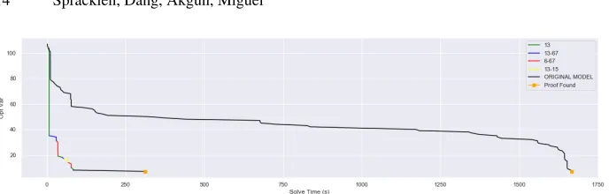
Fig. 4: Objective value progression from the unstreamlined model compared with its progression under the UCB selection method for a representative SONET instance.

optimality. In contrast to the lexicographic methods, which only move on to the next streamlined model when the search space of the current one is exhausted, UCB benefits from its ability to sample the entire streamliner portfolio. After the initial exploration phase, where each streamliner is given its initial application, UCB then selects stream-liners based upon the observed rewards. Its main advantage is the ability to balance the exploration and exploitation of the streamlined models in the portfolio.

It is not always the case that the objective is found purely through the application of one streamliner. For SONET, on average three streamliners are used across the 50 test instances to arrive at the optimal objective value. Access to the whole portfolio allows UCB to descend upon the optimal objective value more quickly and is one reason for its success. The application of several different streamliners at different time points can be used to reduce the bound of the objective in an effective manner as per Figure 4.

The UCB algorithm exploits the streamliners that have previously been shown to produce an improvement in the objective value. This can be very clearly shown from Figure 4 where for an instance from SONET the streamliners 13, 13-67 and 6-671_(explained

in Table 2) improve the objective multiple times during the course of the selection pro-cess. This is due to the fact that UCB is continuing to exploit those streamliners as previously they had success. However, it is also crucial to continually explore the port-folio in an attempt to find streamliners that did not initially have success but may do after a certain number of iterations. Streamliner 13-15 is an example of such a case.

8.2 Time Allocated to the Streamliner Portfolio: Discussion

From Table 5 it can be seen that the T imeT otal parameter as defined in Algorithms 1 and 2 can have a large impact on the overall performance of the selection method. There is a general trend (excluding MEB which will be discussed separately) that as the T imeT otal increases the time both to find and prove the optimal objective value increases. This may seem puzzling initially: if using aT imeT otal of 30s reduces the time to find the optimal objective value to a certain extent, it might be expected that aT imeT otal of 300s will do equally well. However, there are two things to consider. First, streamliners from the portfolio are not guaranteed to preserve the optimal value and so there is the potential for an optimality gap between what the streamliners can

find and the true optimal of the instance. Therefore, the true optimal is only found after the switch to the unstreamlined model occurs. Second, on average the streamliners converge upon their optimal value in a very short period of time, 17s, 7s and 12s for SONET, MEB and PPP respectively. By increasing theT imeT otalparameter it delays the point at which the switch occurs to the unstreamlined model which in turn delays the point at which the true optimal is found. However, for MEB theT imeT otaldoes not have a large impact on performance and this is due to the fact that the streamliners in the portfolio generally exhaust their search space very quickly. Hence, the whole portfolio can be traversed beforeT imeT otalis reached and so the time at which the switch to the unstreamlined model occurs is generally the same across all parameter settings.

The increase in time to prove optimality occurs as if theTtotalparameter is set too large then when the optimal value is found at timeTopt, the whole duration fromTopt→ Ttotal is spent proving the optimality of that solution in the streamlined subspaces. Since proving optimality with respect to the streamliners does not prove optimality on the unstreamlined model and so the whole time fromTopt→Ttotalis wasted.

9

Conclusion and Future Work

We have presented the first automated approach to generating streamliners automati-cally for optimisation problems, and for their selection and scheduling when employed on unseen instances. On three quite different problem classes the results are very en-couraging, with vastly reduced effort both to find and to prove optimal objective values. An important question we plan to investigate further is the applicability of our method to identify in which contexts our streamliner can and cannot help. In the context of optimisation the benefit of streamlining lies in the early identification of the optimal, or at least high quality, values for the objective. Where an unstreamlined model is able to identify the optimal value quickly, the benefit of streamlining will be limited. When considering satisfaction problems, however, streamlining can be used throughout the search and we will compare the portfolio approach developed herein with the single selection provided by the method presented in Spracklen et al. [32].

Furthermore, there are several methods for devising good search strategies for con-strained optimisation problems. Recent research suggest using machine learning to de-sign a promising search ordering [8], using solution density as a heuristic indicator [31] and a number of value ordering heuristics to find good solutions early [30,11]. Stream-lining constraints can potentially be used in combination with the existing methods for devising good variable and value selection heuristics to achieve even better results.

Acknowledgements

References

1. Akg¨un, ¨O.: Extensible automated constraint modelling via refinement of abstract problem specifications. Ph.D. thesis, University of St Andrews (2014)

2. Akg¨un, ¨O., Dang, N., Miguel, I., Salamon, A.Z., Stone, C.: Instance generation via generator instances. In: International Conference on Principles and Practice of Constraint Program-ming. Springer (2019)

3. Akg¨un, ¨O., Gent, I.P., Jefferson, C., Miguel, I., Nightingale, P.: Breaking conditional sym-metry in automated constraint modelling with Conjure. In: ECAI. pp. 3–8 (2014)

4. Auer, P., Cesa-Bianchi, N., Fischer, P.: Finite-time analysis of the

mul-tiarmed bandit problem. Machine Learning 47(2), 235–256 (May 2002).

https://doi.org/10.1023/A:1013689704352

5. Browne, C., Powley, E., Whitehouse, D., Lucas, S., Cowling, P.I., Tavener, S., Perez, D., Samothrakis, S., Colton, S., et al.: A survey of monte carlo tree search methods. IEEE Trans-actions on Computational Intelligence and AI (2012)

6. Burke, D.A., Brown, K.N.: CSPLib problem 048: Minimum energy broadcast (meb). http: //www.csplib.org/Problems/prob048

7. Charnley, J., Colton, S., Miguel, I.: Automatic generation of implied constraints. In: ECAI. vol. 141, pp. 73–77 (2006)

8. Chu, G., Stuckey, P.J.: Learning value heuristics for constraint programming. In: Interna-tional Conference on AI and OR Techniques in Constriant Programming for Combinatorial Optimization Problems. pp. 108–123. Springer (2015)

9. Colton, S., Miguel, I.: Constraint generation via automated theory formation. In: Inter-national Conference on Principles and Practice of Constraint Programming. pp. 575–579. Springer (2001)

10. Dunlop, F., Enright, J., Jefferson, C., McCreesh, C., Prosser, P., Trimble, J.: Expression of graph problems in a high level modelling language. In: Proceedings of the International Workshop on Graphs and Constraints (2018)

11. Fages, J.G., Prud’Homme, C.: Making the first solution good! In: 2017 IEEE 29th Interna-tional Conference on Tools with Artificial Intelligence (ICTAI). pp. 1073–1077. IEEE (2017) 12. Frisch, A.M., Grum, M., Jefferson, C., Hern´andez, B.M., Miguel, I.: The essence of essence.

Modelling and Reformulating Constraint Satisfaction Problems p. 73 (2005)

13. Frisch, A.M., Grum, M., Jefferson, C., Hern´andez, B.M., Miguel, I.: The design of essence: A constraint language for specifying combinatorial problems. In: IJCAI. vol. 7, pp. 80–87 (2007)

14. Frisch, A.M., Harvey, W., Jefferson, C., Mart´ınez-Hern´andez, B., Miguel, I.: Essence: A con-straint language for specifying combinatorial problems. Concon-straints13(3), 268–306 (2008) 15. Frisch, A.M., Jefferson, C., Miguel, I.: Symmetry breaking as a prelude to implied

con-straints: A constraint modelling pattern. In: ECAI. vol. 16, p. 171 (2004)

16. Frisch, A.M., Miguel, I., Walsh, T.: Symmetry and implied constraints in the steel mill slab design problem. In: Proc. CP01 Workshop on Modelling and Problem Formulation (2001) 17. Frisch, A.M., Miguel, I., Walsh, T.: Cgrass: A system for transforming constraint satisfaction

problems. In: Recent Advances in Constraints, pp. 15–30. Springer (2003)

18. Gent, I.P., Jefferson, C., Kotthoff, L., Miguel, I., Moore, N.C., Nightingale, P., Petrie, K.E.: Learning when to use lazy learning in constraint solving. In: ECAI. pp. 873–878. Citeseer (2010)

19. Gent, I.P., Jefferson, C., Miguel, I.: Minion: A fast scalable constraint solver. In: ECAI. vol. 141, pp. 98–102 (2006)

21. Kocsis, L., Szepesv´ari, C.: Bandit based Monte-Carlo planning. In: ECML. pp. 282–293. LNCS 4212, Springer (2006). https://doi.org/10.100711871842 29

22. Kouril, M., Franco, J.: Resolution tunnels for improved sat solver performance. In: In-ternational Conference on Theory and Applications of Satisfiability Testing. pp. 143–157. Springer (2005)

23. Le Bras, R., Gomes, C.P., Selman, B.: On the erd˝os discrepancy problem. In: International Conference on Principles and Practice of Constraint Programming. pp. 440–448. Springer (2014)

24. LeBras, R., Gomes, C.P., Selman, B.: Double-wheel graphs are graceful. In: IJCAI. pp. 587– 593 (2013)

25. L´opez-Ib´a˜nez, M., Dubois-Lacoste, J., C´aceres, L.P., Birattari, M., St¨utzle, T.: The irace package: Iterated racing for automatic algorithm configuration. Operations Research Per-spectives3, 43–58 (2016)

26. Munos, R.: From bandits to Monte-Carlo tree search: The optimistic principle applied to optimization and planning. FTML7(1), 1–129 (2014). https://doi.org/10.1561/2200000038 27. Nethercote, N., Stuckey, P.J., Becket, R., Brand, S., Duck, G.J., Tack, G.: Minizinc: Towards

a standard cp modelling language. In: International Conference on Principles and Practice of Constraint Programming. pp. 529–543. Springer (2007)

28. Nightingale, P.: CSPLib problem 056: Synchronous optical networking (sonet) problem. http://www.csplib.org/Problems/prob056

29. Nightingale, P., Akg¨un, O., Gent, I.P., Jefferson, C., Miguel, I., Spracklen, P.: Automati-cally improving constraint models in Savile Row. Artificial Intelligence251, 35–61 (2017). https://doi.org/10.1016/j.artint.2017.07.001

30. Palmieri, A., Perez, G.: Objective as a feature for robust search strategies. In: International Conference on Principles and Practice of Constraint Programming. pp. 328–344. Springer (2018)

31. Pesant, G.: Counting-based search for constraint optimization problems. In: Thirtieth AAAI Conference on Artificial Intelligence (2016)

32. Spracklen, P., Akg¨un, ¨O., Miguel, I.: Automatic generation and selection of streamlined con-straint models via monte carlo search on a model lattice. In: International Conference on Principles and Practice of Constraint Programming. pp. 362–372. Springer (2018)

33. Walsh, T.: CSPLib problem 013: Progressive party problem. http://www.csplib.org/ Problems/prob013

34. Wang, W., Sebag, M.: Hypervolume indicator and dominance reward based multi-objective monte-carlo tree search. Machine learning92(2-3), 403–429 (2013)