A tensor based selection hyper heuristic for cross domain heuristic search

(1)

A Tensor-based Selection Hyper-heuristic for

Cross-domain Heuristic Search

Shahriar Asta, Ender ¨Ozcan

ASAP Research Group School of Computer Science

University of Nottingham NG8 1BB, Nottingham, UK

Abstract

Hyper-heuristics have emerged as automated high level search methodologies

that manage a set of low level heuristics for solving computationally hard

prob-lems. A generic selection hyper-heuristic combines heuristic selection and move

acceptance methods under an iterative single point-based search framework. At

each step, the solution in hand is modiﬁed after applying a selected heuristic and

a decision is made whether the new solution is accepted or not. In this study,

we represent the trail of a hyper-heuristic as a third order tensor. Factorization

of such a tensor reveals the latent relationships between the low level heuristics

and the hyper-heuristic itself. The proposed learning approach partitions the

set of low level heuristics into two equal subsets where heuristics in each subset

are associated with a separate move acceptance method. Then a multi-stage

hyper-heuristic is formed and while solving a given problem instance,

heuris-tics are allowed to operate only in conjunction with the associated acceptance

method at each stage. To the best of our knowledge, this is the ﬁrst time tensor

analysis of the space of heuristics is used as a data science approach to improve

the performance of a hyper-heuristic in the prescribed manner. The empirical

results across six diﬀerent problem domains from a benchmark indeed indicate

the success of the proposed approach.

Email addresses: sba@cs.nott.ac.uk(Shahriar Asta),Ender.Ozcan@nottingham.ac.uk

(2)

Keywords: Hyper-heuristic, Data Science, Machine Learning, Move

Acceptance, Tensor Analysis, Algorithm Selection

1. Introduction

Hyper-heuristics have emerged as eﬀective and eﬃcient methodologies for

solving hard computational problems. They perform search over the space

formed by a set of low level heuristics, rather than solutions directly [49]. Burke

et al. [13] deﬁned a hyper-heuristic asa search method or learning mechanism

for selecting or generating heuristics to solve computational search problems.

Hyper-heuristics are not allowed to access problem domain speciﬁc information.

It is assumed that there is a conceptual barrier between the hyper-heuristic

level and problem domain where the low level heuristics, solution

representa-tion, etc. reside. This speciﬁc feature gives hyper-heuristics an advantage of

being more general than the existing search methods, since the same

hyper-heuristic methodology can be reused for solving problem instances even from

diﬀerent domains. More on hyper-heuristics can be found in [12, 16, 49]. The

focus of this paper is on selection hyper-heuristics which, often operate under a

single point based search framework by improving an initially created solution

iteratively, exploiting the strengths of multiple low level heuristics. At each

step, a complete solution is updated forming a new solution using a selected

heuristic and this new solution is considered for use in the next step via a move

acceptance method.

There are some recent studies indicating the eﬀectiveness and potential of

mixing multiple move acceptance methods under a selection hyper-heuristic

framework. Kheiri and ¨Ozcan [28] described a bi-stage hyper-heuristic which

allows improving and equal moves only in the ﬁrst stage while a naive move

acceptance method allows worsening moves in the following stage. Ozcan et¨

al. [47] recently combined diﬀerent move acceptance methods and tested

dif-ferent group decision making strategies as a part of selection hyper-heuristics.

(3)

selection hyper-heuristic framework could yield a better running time on some

benchmark functions [36]. Machine learning techniques, such as reinforcement

learning and learning classiﬁer systems have been used as a component of

se-lection hyper-heuristics since the early ideas have emerged [23]. In this study,

we propose a multi-stage selection hyper-heuristic, hybridizing two simple move

acceptance methods, which is signiﬁcantly improved by the use of a machine

learning technique, namely tensor analysis [40].

In the proposed approach, we represent the trail of a selection hyper-heuristic

as a 3rd_{order tensor. Tensor analysis is performed during the search process to}

detect the latent relationships between the low level heuristics and the

hyper-heuristic itself. The feedback is used to partition the set of low level hyper-heuristics

into two equal subsets where heuristics in each subset are associated with a

sep-arate move acceptance method. Then a multi-stage hyper-heuristic combining a

random heuristic selection with two simple move acceptance methods is formed.

While solving a given problem instance, heuristics are allowed to operate only

in conjunction with the corresponding move acceptance method at each

alter-nating stage. This overall search process can be considered as a generalized and

a non-standard version of the iterated local search [38] approach in which the

search process switches back and forth between diversiﬁcation and

intensiﬁca-tion stages. More importantly, the heuristics (operators) used at each stage are

ﬁxed before each run on a given problem instance via the use of tensors. To

the best of our knowledge, this is the ﬁrst time tensor analysis of the space of

heuristics is used as a data science approach to improve the performance of a

selection hyper-heuristic in the prescribed manner. The empirical results across

six diﬀerent problem domains from a benchmark indicate the success of the

proposed hyper-heuristic mixing diﬀerent acceptance methods.

This paper is organized as follows. An overview of hyper-heuristics, together

with the description of the benchmark framework used in this paper is given

in Section 2. Section 3 includes a description of the data analysis method we

have used in our study. Section 4 discusses a detailed account of our framework

(4)

5. Finally, conclusion is provided in Section 6.

2. Selection Hyper-heuristics

A hyper-heuristic either selects from a set of available low level heuristics

or generates new heuristics from components of existing low level heuristics

to solve a problem, leading to a distinction betweenselection and generation

hyper-heuristic, respectively [13]. Also, depending on the availability of feedback

from the search process, hyper-heuristics can be categorized aslearning and

no-learning. Learning hyper-heuristics can be further categorized into online and

oﬄine methodologies depending on the nature of the feedback. Online

hyper-heuristics learnwhilesolving a problem whereas oﬄine hyper-heuristics process

collected data gathered from training instances prior to solving the problem.

The framework proposed in this paper is a single point based search algorithm

which ﬁts best in the online learning selection hyper-heuristic category.

A selection hyper-heuristic has two main components: heuristic selection

and move acceptance methods. While the task of the heuristic selection is to

choose a low level heuristic at each decision point, the move acceptance method

accepts or rejects the resultant solution produced after the application of the

chosen heuristic to the solution in hand. This decision requires measurement

of the quality of a given solution using an objective (evaluation, ﬁtness, cost,

or penalty) function. Over the years, many heuristic selection and move

ac-ceptance methods have been proposed. A survey on hyper-heuristics including

their components can be found in [12, 49].

2.1. Heuristic Selection and Move Acceptance Methodologies

In this section, we describe some of the basic and well known heuristic

selec-tion approaches. [20, 21] are the earliest studies testing simple heuristic selecselec-tion

methods as a selection hyper-heuristic component. One of the most basic and

preliminary approaches to select low level heuristics is the Simple Random (SR)

approach requiring no learning at all. In SR, heuristics are chosen and

(5)

is applied repeatedly until the point in which no improvement is achieved, the

heuristic selection mechanism is Random Gradient. Also, when all low level

heuristics are applied and the one producing the best result is chosen at each

iteration, the selection mechanism is said to be greedy. The heuristic selection

mechanisms discussed so far do not employ learning. There are also many

se-lection mechanisms which incorporate learning mechanisms. Choice Function

(CF) [20, 22, 51] is one of the learning heuristic selection mechanisms which has

been shown to perform well. This method is a score based approach in which

heuristics are adaptively ranked based on a composite score. The composite

score itself is based on few criteria such as: the individual performance proﬁle

of the heuristic, the performance proﬁle of the heuristic combined with other

heuristics and the time elapsed since the last call to the heuristic. The ﬁrst two

components of the scoring system emphasise on the recent performance while

the last component has a diversifying eﬀect on the search.

In [43], a Reinforcement Learning (RL) approach has been introduced for

heuristic selection. Weights are assigned to heuristics and the selection process

takes weight values into consideration to favour some heuristics to others. In

[14], the RL approach is hybridized with Tabu Search (TS) where the tabu list

of heuristics which are temporarily excluded from the search process is kept

and used. There are numerous other heuristic selection mechanisms. Interested

reader can refer to [12] for further detail.

As for the move acceptance component, currently, there are two types of

move acceptance methods: deterministic and non-deterministic [12]. The

de-terministic move acceptance methods make the same decision (as for

accep-tion/rejection of the solution provided by a heuristic) irrespective of the

de-cision point. In contrast to deterministic move acceptance, non-deterministic

acceptance strategies incorporate some level of randomness resulting in diﬀerent

decisions for the same decision point. The non-deterministic move acceptance

methods almost always are parametric, utilizing parameters such as time or

current iteration.

(6)

acceptance methods, such as Improvement Only (IO), Improvement and Equal

(IE) and Naive Acceptance (NA) [20]. The IO acceptance criteria only accepts

solutions which oﬀer an improvement in the current objective value. The IE

method accepts all solutions which result in objective value improvement. It

also accepts solutions which do not change the current objective value. Both

IO and IE strategies are deterministic strategies. The NA strategy is a

non-deterministic approach which accepts all improving and equal solutions by

de-fault and worsening solutions with a ﬁxed probability of α. Although there

are more elaborate move acceptance methods, for example, Monte-Carlo based

move acceptance strategy [7], Simulated Annealing [10], Late Acceptance [11],

there is strong empirical evidence that combining simple components under a

selection hyper-heuristic framework with the right low level heuristics could still

yield an improved performance. [46] shows that the performance of a selection

hyper-heuristic could vary if the set of low level heuristics change, as expected.

[29] describes the runner up approach at a high school timetabling competition,

which uses SR as heuristic selection and a move acceptance method with 3

diﬀer-ent threshold value settings. Moreover, there are experimdiﬀer-ental and theoretical

studies showing that mixing move acceptance can yield improved performance

[28, 36, 47]. Hence, in this study, we ﬁx the heuristic selection method as SR and

propose an online learning method to partition the low level heuristics,

predict-ing which ones would perform well with a naive move acceptance method and

assigning the others to IE. Then we mix the move acceptance methods under

a multi-stage selection hyper-heuristic framework invoking only the associated

heuristics when chosen.

2.2. HyFlex and the First Cross-Domain Heuristic Search Challenge (CHeSC

2011)

Hyper-heuristics Flexible Framework (HyFlex) [44] is an interface to

sup-port rapid development and comparison of various hyper/meta-heuristics across

various problem domains. The HyFlex platform promotes the reusability of

(7)

the problem domain via a domain barrier [19] to promote domain-independent

automated search algorithms. Hence, problem domain independent information,

such as the number of heuristics and objective value of a solution, is allowed to

pass through the domain barrier to the hyper-heuristic level (Figure 1). On the

other hand, pieces of problem dependent information, such as, representation

and objective function are kept hidden from the higher level search algorithm.

Restricting the type of information available to the hyper-heuristic to a domain

independent nature is considered to be necessary to increase the level of

gen-erality of a hyper-heuristic over multiple problem domains. This way the same

approach can be applied to a problem from another domain without requiring

any domain expert knowledge or intervention.

Hyper-heuristic

Select a heuristic (ࢎ࢏) based on a selection method and apply it to a given solution (࢙࢐), creating a new solution (࢙࢑).

Domain Barrier

Problem Domain

Accept or reject the new/resultant solution (࢙࢑) based on an acceptance

method.

• Low level heuristics (ࢎ૚, … , ࢎ࢔),

• Solution representation (list of solutions – (࢙૚, … , ࢙࢒)),

• Objective function (f(.)), etc... e.g., [࢏, ࢐, ࢑] e.g., [ࢌ൫࢙࢐൯, ࢌ(࢙࢑)]

ࢎ૚ ࢎ࢏ ࢎ࢔

࢙૚ ࢙࢐ ࢙࢑ ࢙࢒

[image:7.612.194.419.329.481.2]

ࢎ࢏(࢙࢐)

Figure 1: A selection hyper-heuristic framework [19].

HyFlex v1.0 is implemented in Java respecting the interface deﬁnition and

was the platform of choice at a recent competition referred to as the

Cross-domain Heuristic Search Challenge (CHeSC 2011)1. The CHeSC 2011

compe-tition aimed at determining the state-of-the-art selection hyper-heuristic judged

by the median performance of the competing algorithms across thirty problem

instances, ﬁve for each problem domain. Formula 1 scoring system is used to

(8)

assess the performance of hyper-heuristics over problem domains. In formula

1 scoring system, for each instance, the top eight competing algorithms receive

scores of 10,8,6,5,4,3,2 or 1 depending on their rank on a speciﬁc instance.

Remaining algorithms receive a score of 0. These scores are then accumulated to

produce the overall score of each algorithm on all problem instances. The

com-peting algorithms are then ranked according to their overall score. The number

of competitors during the ﬁnal round of the competition was 20. Moreover, a

wide range of problem domains is covered in CHeSC 2011. Consequently, the

results achieved in the competition along with the HyFlex v1.0 platform and

the competing hyper-heuristics currently serve as a benchmark to compare the

performance of novel selection hyper-heuristics.

The CHeSC 2011 problem domains include Boolean Satisﬁability (SAT),

One Dimensional Bin Packing (BP), Permutation Flow Shop (FS), Personnel

Scheduling (PS), Travelling Salesman Problem (TSP) and Vehicle Routing

Prob-lem (VRP). Each domain provides a set of low level heuristics which are

clas-siﬁed as mutation (MU), local search (LS)(also referred to as hill climbing),

Ruin and Re-create (RR) and crossover (XO) heuristics (operators). Each low

level heuristic, depending on it’s nature (i.e. whether it is a mutational or a

local search operator) comes with an adjustable parameter. For instance, in

mutational operators, the mutation density determines the extent of changes

that the selected mutation operator yields on a solution. A high mutation

den-sity indicates wider range of new values that the solution can take, relevant to

its current value. Lower values suggest a more conservative approach where

changes are less inﬂuential. As for thedepthof local search operators, this value

relates to the number of steps completed by the local search heuristic. Higher

values indicate that local search approach searches more neighbourhoods for

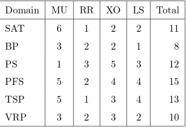
improvement. Table 1 summarizes the low level heuristics for each domain of

CHeSC 2011 and groups them according to their type (e.g. MU, RR, XO and

LS).

The description of each competing hyper-heuristic can be reached from the

(9)

pro-Table 1: The number of diﬀerent types of low level heuristics{mutation (MU), ruin and re-create heuristics (RR), crossover (XO) and local search (LS)} used in each CHeSC 2011 problem domain.

Domain MU RR XO LS Total

SAT 6 1 2 2 11

BP 3 2 2 1 8

PS 1 3 5 3 12

PFS 5 2 4 4 15

TSP 5 1 3 4 13

VRP 3 2 3 2 10

vided in Table 2. The top three selection hyper-heuristics that generalize well

across the CHeSC 2011 problem domains are multi-stage approaches of AdapHH

[41], VNS-TW [27] and ML [33].

3. Tensor Analysis

Tensorsare multidimensional arrays and the orderof a tensor indicates its

dimensionality. Each dimension of a tensor is referred to as a mode. In our

notation, following [31], a boldface Euler script letter, boldface capital letter

and boldface lower-case letter denote a tensor (e.g., T), matrix (e.g.,M) and vector (e.g.,v), respectively. The entries of tensors, matrices and vectors (and scalar values in general) are indexed by italic lower-case letters. For example,

the (p, q, r) entry of a 3rd₋_{order (three dimensional) tensor}_T _{is denoted as}_t pqr.

3.1. Tensor Decomposition (Factorization)

Tensor decomposition (a.k.a tensor factorization) is used in many research

ﬁelds to identify the correlations and relationships among diﬀerent modes of

high dimensional data. The tensor decomposition methods are mainly

gener-alizations of the Singular Value Decomposition (SVD) to higher dimensions.

[image:9.612.213.400.181.310.2]

(10)

[image:10.612.174.437.167.366.2]

Table 2: Rank of each hyper-heuristic (denoted as HH) competed in CHeSC 2011 with respect to their Formula 1 scores.

Rank HH Score Rank HH Score

1 AdapHH 181 11 ACO-HH 39

2 VNS-TW 134 12 GenHive 36.5

3 ML 131.5 13 DynILS 27

4 PHUNTER 93.25 14 SA-ILS 24.25

5 EPH 89.75 15 XCJ 22.5

6 HAHA 75.75 16 AVEG-Nep 21

7 NAHH 75 17 GISS 16.75

8 ISEA 71 18 SelfSearch 7

9 KSATS-HH 66.5 19 MCHH-S 4.75

10 HAEA 53.5 20 Ant-Q 0

(a.k.a PARAFAC or CANDECOMP or CP) [26] and Non-negative Tensor

Fac-torization (NTF) [50] are among numerous facFac-torization methods proposed by

researchers. Tucker decomposition has applications in data compression [57],

dimensionality reduction [56] and noise removal [42] among others. Also CP

decomposition has been used for noise removal and data compression [24]. In

addition, it has a wide range of applications in many scientiﬁc areas such as

Data Mining [8] and telecommunications [34]. There are few other

factoriza-tion methods which mainly originate from CP and/or Tucker methods. Each of

these methods (such as INDSCAL, PARAFAC2 and PARATUCK2) are widely

known in speciﬁc ﬁelds such as chemometrics or statistics. For more details on

these methods the reader is referred to [31]. Also, the studies in [2] and [1]

provide very detailed comparison between factorization methods.

In this study, we have used the CP decomposition method. Furthermore,

we focus on 3rd-order tensors. Assume that we have such tensor denoted byT

(11)

(ALS) algorithm [15, 25], in which tensorT is approximated by another tensor

ˆ

T as in Equation 1.

ˆ

T =

K ∑

k=1

λk ak◦bk◦ck (1)

λk ∈R+, ak ∈RP, bk ∈RQ and ck ∈RR for k= 1· · ·K, where K is the

number of desired components. Each summand (λk ak◦bk◦ck) is called a component while the individual vectors are called factors. λk is the weight of

thekth component. Note that “◦” is the outer product operator. The outer

product of three vectors produces a 3rd_{-order tensor. For instance, given}_K_{= 1,}

Equation 1 reduces to ˆT =λa◦b◦c, in which ˆT is a 3rd_{-order tensor which is} obtained by the outer product of three vectorsa, bandc. Subsequently, each tensor entry, denoted as ˆtpqr is computed through a simple multiplication like

apbqcr.

The outer productak◦bk in Equation 1 quantiﬁes the relationship between the object pairs, i.e., score values indicating the “level of interaction” between

object pairs in component k [31]. The purpose of the ALS algorithm is to

minimize the error diﬀerence between the original tensor and the estimated

tensor, denoted asεas follows:

ε= 1

2||T −

ˆ

T ||2F (2)

where the subscriptF refers to the Frobenious norm. That is:

||T −_{T ||}ˆ 2 F =

P ∑

p=1 Q ∑

q=1 R ∑

r=1 (

tpqr−ˆtpqr )2

(3)

After applying the factorization method, in addition to the CP model, a

measure of how well the original data is described by the factorized tensor can

be obtained. This measure (model fitness), denoted asϕ, is computed using the

following equation:

ϕ= 1−||T −

ˆ

T ||F

||T ||F

(12)

where the valueϕis in the range [0,1]. Theϕvalue is an indicator which shows

how close the approximated tensor is to the original data. In other words, it

measures the proportion of the original data represented in the approximated

tensor ˆT. A perfect factorization (where T = ˆT) results in ϕ = 1, while a

poor factorization results inϕ= 0, hence as theϕ value increases, so does the

factorization accuracy. More on tensor decompositions and their applications

can be found in [31].

As well as representing data in a concise and more generalizable manner

which is immune to data anomalies (such as missing data), tensor factorization

methods oﬀer additional interesting utilities. Those methods allow partitioning

of the data into a set of more comprehensible sub-data which can be of speciﬁc

use depending on the application according to various criteria. For example, in

the ﬁeld of computer vision, [30] and [32] separately show that factorization of

a 3rd_{-order tensor of a video sequence results in some interesting basic factors.}

These basic factors reveal the location and functionality of human body parts

which move synchronously.

3.2. Motivation: Inspirations From Applications of Tensor Analysis

Many problems produce data of a nature which is best described and

repre-sented in high dimensional data structures. However, for the sake of simplicity,

the dimensionality of data is often deliberately reduced. For instance, in face

recognition, the set of images of various individuals constitutes a three

dimen-sional data structure where the ﬁrst two dimensions are thexandycoordinates

of each pixel in each image and the third dimension is the length of the dataset.

This is while, in classical face recognition (like the eigenface method), each face

image is reduced to a vector by concatenating the pixel rows of the image.

Con-sequently, the dataset, which is 3D (or maybe higher) in nature, is reduced to a

2D dataset for further processing. However, [56] shows that by sticking to the

original dimensionality of the data and representing the dataset as a 3rd_-order

tensor, better results are achieved in terms of the recognition rate. This is due

(13)

information regarding the dependencies, correlation and useful redundancies in

the feature space [39]. On the other hand, representing the data in its natural

high dimensional form helps with preserving the latent structures in the data.

Employing tensor analysis tools helps in capturing those latent relationships

([4], [5]). Similar claims have been registered in various research areas such

as human action recognition in videos [32], hand written digit recognition [59],

image compression [60], object recognition [58], gait recognition [54],

Electroen-cephalogram (EEG) classiﬁcation [37], Anomaly detection in streaming data

[52], dimensionality reduction [39], tag recommendation systems [48] and Link

Prediction on web data [3].

The search history formed by a heuristic, metaheuristic or hyper-heuristic

methodology constitutes a multi-dimensional data. For example, when

popu-lations of several generations of individuals in a Genetic Algorithm (GA) are

put together, the emerging structure representing the solutions and associated

objective values changing in time is a 3rd_{-order tensor. Similarly, the interaction}

between low level heuristics as well as the interaction between those low level

heuristics and the acceptance criteria under a selection hyper-heuristic

frame-work are a couple of examples of various modes of functionality in a hypothetical

tensor representing the search history.

Some selection hyper-heuristics, such as reinforcement-based hyper-heuristics

or hyper-heuristics embedding late acceptance or tabu search components do

use some of the search history selectively. Their performance is usually

con-ﬁned with memory restrictions. Moreover, the memory often contains raw data,

such as objective values or visited states and those components ignoring the

hidden clues and information regarding the choices that inﬂuences the overall

performance of the approach in hand.

In this study, we use a 3rd_{-order tensor to represent the search history of}

a hyper-heuristic. The ﬁrst two modes are indexes of subsequent low level

heuristics selected by the underlying hyper-heuristic while the third mode is the

time. Having such a tensor ﬁlled with the data acquired from running the

(14)

level heuristics which are performing well with the underlying hyper-heuristic

and acceptance criteria. This is very similar to what has been done in [32],

except that, instead of examining the video of human body motion and looking

for diﬀerent body parts moving in harmony, we examine the trace of a

hyper-heuristic (body motion) and look for low level hyper-heuristics (body parts) performing

harmoniously. Naturally, our ultimate goal is to exploit this knowledge for

improving the search process.

4. A Tensor-based Selection Hyper-Heuristic Approach Hybridizing Move Acceptance

The low level heuristics in HyFlex are divided into four groups as described in

Section 2. The heuristics belonging to the mutational (MU), ruin-recreate (RR)

and local search (LS) groups are unary operators requiring a single operand.

This is while, the crossover operators have two operands requiring two

candi-date solutions to produce a new solution. In order to maintain simplicity as

well as coping with the single point search nature of our framework, crossover

operators are ignored in this study and MU, RR and LS low level heuristics

are employed. The set of all available heuristics (except crossover operators)

for a given problem domain is denoted by a lower-case bold and italic letterh

throughout the paper. Moreover, from now on, we refer to our framework as

Tensor Based Hybrid Acceptance Hyper-heuristic (TeBHA-HH) which consists

of ﬁve consecutive phases: (i) noise elimination (ii) tensor construction, (iii)

ten-sor factorization, (iv) tenten-sor analysis, and (v) hybrid acceptance as illustrated in

Figure 2. The noise elimination ﬁlters out a group of low level heuristics fromh

and then a tensor is constructed using the remaining set of low level heuristics,

denoted ash−. After tensor factorization, sub-data describing the latent

rela-tion between low level heuristics is extracted. This informarela-tion is used to divide

the low level heuristics into two partitions: hN A, hIE. Each partition is then

associated with a move acceptance method, that is naive move acceptance with

(15)

equiv-alent to employing two selection hyper-heuristics, Simple Random-Naive move

acceptance (SR-NA) and Simple Random-Improving and Equal (SR-IE). Each

selection hyper-heuristic is invoked in a round-robin fashion for a ﬁxed duration

of time (ts) using only the low level heuristics associated with the move

accep-tance component of the hyper-heuristic at work (hN A and hIE, respectively)

until the overall time limit (Tmax) is reached. This whole process is repeated at

each run while solving a given problem instance. All the problems dealt with

in this study are minimizing problems. A detailed description of each phase is

[image:15.612.153.458.297.484.2]

given in the subsequent sections.

Figure 2: The schematic of our proposed framework.

4.1. Noise Elimination

We model the trace of the hyper-heuristic as a tensor dataset and factorize

it to partition the heuristic space. Tensor representation gives us the power to

analyse the latent relationship between heuristics. But this does not mean that

any level and type of noise is welcome in the dataset. The noise in the dataset

may even obscure the existing latent structures. Thus, reducing the noise is

(16)

framework in which a low level heuristic is chosen randomly, if a heuristic

per-turbs a solution and consistently generates highly worsening solutions, then such

a heuristic is considered as a poor heuristic, causing partial re-starts which is

often not a desirable behaviour. Hence, the tensor dataset produced while such

a heuristic is used can be considerednoisy (noise is generally deﬁned as

unde-sired data) and that heuristic can be treated as source of the noise. Identifying

such heuristics at the start and eliminating them results in a less noisy dataset.

The type of noise happens to be very important in many data mining

tech-niques and tensor factorization is not an exception. CP factorization method

which is one of the most widely used factorization algorithms, assumes a

Gaus-sian type noise in the data. It has been shown that CP is very sensitive to

non-Gaussian noise types [18]. In hyper-heuristics, change in the objective value

after applying each heuristic follows a distribution which is very much

depen-dent on the problem domain and the type of the heuristic, both of which are

unknown to a hyper-heuristic and unlikely to follow a Gaussian distribution.

To the best of our knowledge, while there are not many factorization methods

which deal with various types of noise in general, there is no method tailored

for heuristics. Thus, it is crucial to reduce the noise as much as possible prior

to any analysis of the data. This is precisely the aim of the ﬁrst phase of our

approach.

Excluding the crossover heuristics leaves us with three heuristic groups (MU,

RR and LS). A holistic strategy is used in the noise elimination phase for

get-ting rid of poor heuristics. An overall pre-processing time, denoted as tp is

allocated for this phase. Except the LS group, applying heuristics belonging to

all other groups may lead to worsening solutions. Hence, theworstof the two

remaining heuristic groups (MU and RR) is excluded from the subsequent step

of the experiment. In order to determine the group of low level heuristics to

eliminate, SR-NA is run using the MU and LS low level heuristics for a duration

oftp/2, which is followed by another run using RR and LS low level heuristics

for the same duration. Performing the pre-processing tests in this manner also

(17)

the proposed framework for improvement. During each run, the search process

is initiated using the same candidate solution for a fair comparison. The quality

of the solutions obtained during those two successive runs are then compared.

Whichever group of low level heuristics generates the worst solution under the

described framework gets eliminated. The remaining low level heuristics,

de-noted ash− is then fed into the subsequent phase for tensor construction.

4.2. Tensor Construction and Factorization

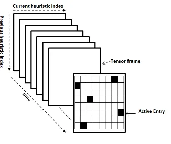
We represent the trail of SR-NA as a 3rd-order tensorT ∈RP×RQ×RRin

this phase, whereP =Q=|h−|is the number of available low level heuristics

andR=N represents the number of tensor frames collected in a given amount

of time. Such a tensor is depicted in Figure 3. The tensorT is a collection of two

dimensional matrices (M) which are referred to astensor frames. A tensor frame is a two dimensional matrix of heuristic indices. Column indices in a tensor

frame represent the index of the current heuristic whereas row indices represent

[image:17.612.224.393.412.555.2]

the index of the heuristic chosen and applied before the current heuristic.

Figure 3: The tensor structure in TeBHA-HH. The black squares (also referred to as active entries) within a tensor frame highlight heuristic pairs invoked subsequently by the underlying hyper-heuristic.

The tensor frame is ﬁlled with binary data as demonstrated in Algorithm 1.

The bulk of the algorithm is the SR-NA hyper-heuristic (starting at the while

(18)

applied to the problem instance (line 14). This action returns a new objective

value fnew which is used together with the old objective value fold to

calcu-late the immediate change in the objective value (δf). The algorithm then

checks ifδf >0 indicating improvement, in which case the solution is accepted.

Otherwise, it is accepted with probability 0.5 (line 21). While accepting the

solution, assuming that the indices of the current and previous heuristics are

hcurrent and hprevious respectively, the tensor frame M is updated symmetri-cally: mhprevious,hcurrent = 1 andmhcurrent,hprevious = 1. The frame entries with

the value 1 are referred to as active entries. At the beginning of each iteration,

the tensor frame M is checked to see if the number of active entries in it has reached a given threshold of⌊|h|/2⌋ (line 5). If so, the frame is appended to

tensor and a new frame is initialized (lines 6 to 9). This whole process is

re-peated until a time limit is reached which the same amount of time allocated

for the pre-processing phase;tp (line 4).

While appending a frame to the tensor, each tensor frame is labelled by the

∆f it yields, where ∆f is the overall change in objective value caused during the

construction of the frame. ∆f is diﬀerent fromδf in the sense that the former

measures the change in objective value inﬂicted by the collective application of

active heuristic indexes inside a frame. The latter is the immediate change in

objective value caused by applying a single heuristic.

The aforementioned process constructs an initial tensor which contains all

the tensor frames. However, we certainly do want to emphasize on intra-frame

correlations as well. That is why, after constructing the initial tensor, the tensor

frames are scanned for consecutive frames of positive labels(∆f >0). In other

words, a tensor frame is chosen and put in the ﬁnal tensor only if it has a

positive label and has at least one subsequent frame with a positive label. The

ﬁnal tensor is then factorized using the CP decomposition to the basic frame

(K= 1 in Equation 1). The following section illustrates how the basic frame is

(19)

Algorithm 1:The tensor construction phase

1 In: h=h−;

2 Initialize tensor frameMto 0;

3 counter= 0;

4 whilet < t_p do

5 if counter=⌊|h|/2⌋then

6 appendMtoT;

7 set frame label to ∆f;

8 Initialize tensor frameMto 0;

9 counter= 0;

10 end

11 hprevious=hcurrent;

12 hcurrent= selectHeuristic(h);

13 fcurrent=fnew;

14 fnew=applyHeuristic(hcurrent);

15 δf =fcurrent−fnew;

16 if δf >0then

17 mhprevious,hcurrent= 1;

18 counter+ +;

19 else

20 if probability >0.5 then

21 mhprevious,hcurrent= 1;

22 if δf = 0 then

23 m_h_current_,h_previous = 1;

24 end

25 counter+ +;

26 end

27 end

(20)

4.3. Tensor Analysis: Interpreting The Basic Frame

Following the tensor factorization process, the tensor is decomposed into

basic factors. K= 1 in our case, thus, the Equation 1 reduces to the following

equation:

ˆ

T =λa◦b◦c (5)

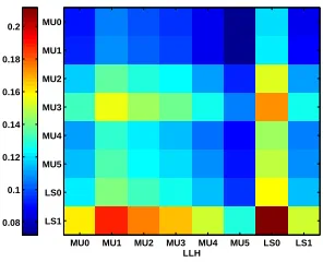
The outer product in the form a◦b produces a basic frame which is a matrix. Assume that, in line with our approach, we have constructed a tensor

from the data obtained from the hyper-heuristic search for a given problem

instance in a given domain which comes with 8 low level heuristics, 5 of them

being mutation and 2 of them being local search heuristics. Moreover, the

factorization of the tensor produces a basic frame as illustrated in Figure 4. The

values inside the basic frame are the scores of each pair of low level heuristics

when applied together. Since we are interested in pairs of heuristics which

perform well together, we locate the pair which has the maximum value (score).

In this example, the pair (LS0, LS1) performs the best since the score for that

pair is the highest. We regard these two heuristics as operators which perform

well with the NA acceptance mechanism under the selection hyper-heuristic

framework. The heuristics in the column corresponding to this maximum pair

are then sorted to determine a ranking between the heuristics. Since heuristics

LS0 andLS1 are already the maximizing pair, they are considered to be the top

two elements of this list. In the basic frame of Figure 4 the sorted list is then

(LS0,LS1,M U3,M U2,M U5,M U4,M U1,M U0). The top/ﬁrst⌊|h|/2⌋elements

of this list is then selected as those heuristics which perform well under NA

acceptance mechanism (hN A). The remaining low level heuristics including the

eliminated heuristics (e.g., RR heuristics) are associated with IE (hIE).

4.4. Final Phase: Hybrid Acceptance

Selection hyper-heuristics have been designed mainly in two ways: ones

which require the nature of low level heuristics to be known, while the

(21)

LLH

MU0 MU1 MU2 MU3 MU4 MU5 LS0 LS1

MU0

MU1

MU2

MU3

MU4

MU5

LS0

LS1 0.08

[image:21.612.230.378.131.251.2]

0.1 0.12 0.14 0.16 0.18 0.2

Figure 4: A sample basic frame. Each axis of the frame represents heuristic indexes. Higher scoring pairs of heuristics are darker in color.

that whether a given low level heuristic is mutational (or ruin-recreate) or local

search is known, since they use only the relevant heuristics to be invoked at

diﬀerent parts of those algorithms. On the other hand, AdapHH [41] operated

without requiring that information. Our hyper-heuristic approach is of former

type. Additionally, we ignore the crossover heuristics as many of the other

previously proposed hyper-heuristics.

In this paper, we have considered a multi-stage selection hyper-heuristic

which uses simple random heuristic selection and hybridizes the move

accep-tance methods, namely NA and IE. These selection hyper-heuristic components

with no learning are chosen simply to evaluate the strength of the tensor based

approach as a machine learning technique under the proposed framework. This

is the ﬁrst time the proposed approach has been used in heuristic search as a

component of a selection hyper-heuristic. In this phase, the best solution found

so far is improved further using the proposed hyper-heuristic which switches

between SR-NA and SR-IE. Since the same simple random heuristic selection

method is used at all times, the proposed selection hyper-heuristic, in a way,

hy-bridizes the move acceptance methods under the multi-stage framework. Each

acceptance method is given the same amount of time;tsto run. SR-NA operates

(22)

search process continues until the time allocated to the overall hyper-heuristic

(Algorithm 2) expires.

There are many cases showing that explicitly enforcing diversiﬁcation

(ex-ploration) and intensiﬁcation (exploitation) works in heuristic search. For

exam-ple, there are many applications indicating the success of iterated local search

(ILS) [38] and memetic algorithms (MAs) [17, 45]. Those metaheuristic

ap-proaches explicitly enforce the successive use of mutational and local search

heuristics/operators in an attempt to balance diversiﬁcation and intensiﬁcation

processes. The choice of NA and IE is also motivated by the reason that under

the proposed framework, SR-NA can be considered as a component allowing

diversiﬁcation, while SR-IE focuses on intensiﬁcation. Similar to ILS and MAs,

the proposed approach also explicitly maintains the balance between

diversifica-tion and intensificadiversifica-tion with the differences that SR-NA and SR-IE is employed

in stages (not at each iteration) for a ﬁxed period of time during the search

process and the best subset of heuristics/operators that interact well to be used

in a stage is determined through learning by the use of tensor analysis. Putting

low level heuristics performing poorly with SR-NA under SR-IE somewhat

en-sures that those low level heuristics cause no harm misleading the overall search

process.

5. Experimental Results

The experiments are performed on an Intel i7 Windows 7 machine (3.6 GHz)

with 16 GB RAM. This computer was given 438 seconds (corresponding to 600

nominal seconds on the competition machine) as the maximum time allowed

(Tmax) per instance by the benchmarking tool provided by the CHeSC 2011

organizers. This is to ensure a fair comparison between various algorithms. We

used the Matlab Tensor Toolbox [9] 2 for tensor operations. The HyFlex, as

well as the implementation of our framework is in Java. Hence, subsequent to

2

(23)

Algorithm 2: Tensor Based Hyper-heuristic with Hybrid Acceptance Strategy

1 leth be the set of all low level heuristics;

2 lettbe the time elapsed so far;

3 h−_x = exclude XO heuristics;

4 h− = preProcessing(tp,h−x);

5 T = constructTensor(tp,h−);

6 a,b,c= CP(T, K = 1) , B=a◦b; 7 x, y=max(B);

8 hs=sort(Bi=1:_|h−_|,y);

9 hN A= (hs)i=1:_⌊|hs|/2⌋ , hIE=h

−

x −hN A;

10 whilet < Tmax do

11 if acceptance=N Athen

12 h = selectRandomHeuristic(h_{N A});

13 else

14 h = selectRandomHeuristic(hIE);

15 end

16 snew, fnew= applyHeuristic(h, scurrent);

17 δ=fold−fnew;

18 updateBest(δ,fnew);

19 if acceptanceT imer≥ts then

20 toggle acceptance mechanism;

21 end

22 if switch=truethen

23 s_new, s_old=NA(s_new, f_new, s_current, f_current) ;

24 else

25 snew, sold=IE(snew, fnew, scurrent, fcurrent);

26 end

(24)

tensor construction phase, Matlab is called from within Java to perform the

factorization task. Throughout the paper, whenever a speciﬁc setting of the

TeBHA-HH framework is applied to a problem instance, the same experiment

is repeated for 31 times, unless mentioned otherwise.

5.1. Experimental Design

One of the advantages of the TeBHA-HH framework is that it has

consid-erably few parameters. To be more precise there are two parameters governing

the performance of our tensor based hybrid acceptance approach. The ﬁrst

pa-rameter is the time allocated to pre-processing and tensor construction phases.

This time boundary is equal for both phases and is denoted astp. The second

parameter is the time allowed to an acceptance mechanism in the ﬁnal phase.

During the ﬁnal phase, the proposed selection hyper-heuristic switches between

the two move acceptance methods (and their respective heuristic groups). Each

move acceptance method is allowed to be in charge of solution acceptance for a

speciﬁc time which is the second parameter and is denoted asts.

Note that all our experiments are conducted on the set of instances provided

by CHeSC 2011 organizers during the ﬁnal round of the competition. HyFlex

contains more than a dozen of instances per problem domain. However, during

the competitions 5 instances per domain were utilized. These are the set of

instances which were employed in this paper.

A preliminary set of experiments are performed in order to show the need for

the noise elimination phase and more importantly to evaluate the performance

of Automatic Noise Elimination (AUNE) in relation to the factorization process

ﬁxing tp and ts values. This preliminary experiment along with experiments

involving evaluation of various values of parameterstpandtsare only conducted

on the ﬁrst instance of each problem domain. After this initial round of tests

in which the best performing values for the parameters of the framework are

determined, a second experiment, including all the competition instances is

conducted and the results are compared to that of the CHeSC 2011 competitors.

(25)

valuesnil(0), 500, 1000 and 1500 milliseconds are experimented.

5.2. Pre-processing Time

The experiments in this section concentrates on the impact of the time (tp)

given to the ﬁrst two phases (noise elimination and tensor construction) on the

performance of the overall approach. During the ﬁrst phase in all of the runs,

theRRgroup of heuristics have been identiﬁed as source of noise for Max-SAT

and VRP instances. This is while,M U has been identiﬁed as source of noise

for BP, FS and TSP instances. As for the PS domain, due to small number of

frames collected (which is a result of slow speed of heuristics in this domain),

nearly half of the time RR has been identiﬁed as the source of noise. In the

remaining runsM U group of heuristics are excluded as noise. Our experiments

show that for a given instance, the outcome of the ﬁrst phase is persistently

similar for diﬀerent values oftp.

Thetpvalue also determines the number of tensor frames recorded during the

tensor construction phase. Hence, we would like to investigate how many tensor

frames areadequate in the second phase. We expect that an adequate number

of frames would result in a stable partitioning of the heuristic space regardless

of how many times the algorithm is run on a given instance. As mentioned

in Section 5.1, three values (15,30 and 60 seconds) are considered. Rather

than knowing how the framework performs in the maximum allowed time, we

are interested to know whether diﬀerent values for tp result in tremendously

diﬀerent heuristic subsets at the end of the ﬁrst phase. Thus, in this stage of

experiments, for a given value oftp, we run the ﬁrst two phases only. That is, for

a given value oftpwe run the simple noise elimination algorithm. Subsequently,

we construct the tensor for a given instance. At the end of these ﬁrst two phases,

the contents ofhN A and hIE are recorded. We do this for 100 runs for each

instance. At the end of the runs for a given instance, a histogram of the selected

heuristics is constructed. The histograms belonging to a speciﬁc instance and

achieved for various values oftp are then compared to each other. Figures 5

(26)

6 problem domains in HyFlex.

The histograms show the number of times a given heuristic is chosen ashN A

orhIE within the runs. For instance, looking at the histograms corresponding

to the Max-SAT problem (Figures 5(a), 5(b) and 5(c)), one could notice that

the heuristicLS1 is always selected ashN A in all the 100 runs. This is while

RR0 is always assigned tohIE. The remaining heuristics are assigned to both

sets although there is a bias towardshN Ain case of heuristicsM U2, M U3 and

M U5. A similar bias towardshIEis observable for heuristicsM U0, M U1, M U4

andLS0. This shows that the tensor analysis together with noise elimination

adapts its decision based on the search history for some heuristics while for

some other heuristics deﬁnite decisions are made. This adaptation is indeed

based on several reasons. For one thing, some heuristics perform very similar to

each other leading to similar traces. This is while, their performance patterns,

though similar to each other, varies in each run. Moreover, there is an indication

that there is no unique optimal subgroups of low level heuristics under a given

acceptance mechanism and hyper-heuristic. There indeed might exists several

such subgroups. For instance, there are two (slightly) diﬀerent NA subgroups

(hN A={M U2, M U5, LS0, LS1}andhN A={M U2, M U3, LS0, LS1}) for the

Max-SAT problem domain which result in the optimal solution (f = 0). This

is strong evidence supporting our argument about the existence of more than

one useful subgroups of low level heuristics. Thus, it only makes sense if the

factorization method, having several good options (heuristic subsets), chooses

various heuristic subsets in various runs.

Interestingly, RR0 and LS1 are diversifying and intensifying heuristics

re-spectively. Assigning RR0 to hIE means that the algorithm usually chooses

diversifying operations that actually improves the solution. A tendency to such

assignments is observable for other problem instances, though not as strict as

it is for BP and Max-SAT problem domains. While this seems to be a very

conservative approach towards the diversifying heuristics, as we will see later

in this section, it often results in a good balance between intensiﬁcation and

(27)

MU0MU1MU2MU3MU4MU5RR0 LS0 LS1 0 20 40 60 80 100 120 heuristic index

number of runs

NA IE

(a) Max-SAT,tp= 15sec

MU0MU1MU2MU3MU4 MU5RR0LS0 LS1 0 20 40 60 80 100 120 heuristic index

number of runs

NA IE

(b) Max-SAT,tp= 30sec

MU0MU1MU2MU3MU4MU5RR0 LS0 LS1 0 20 40 60 80 100 120 heuristic index

number of runs

NA IE

(c) Max-SAT,tp= 60sec

MU0 RR0 RR1 MU1 LS0 MU2 LS1 0 20 40 60 80 100 120 heuristic index

number of runs

NA IE

(d) BP,tp= 15sec

number of runs

NA IE

(e) BP,tp= 30sec

number of runs

NA IE

(f) BP,tp= 60sec

LS0 LS1 LS2 LS3 LS4RR0RR1RR2MU0 0 20 40 60 80 100 120 heuristic index

number of runs

NA IE

(g) PS,tp= 15sec

LS0 LS1 LS2 LS3 LS4 RR0RR1RR2MU0 0 20 40 60 80 100 120 heuristic index

number of runs

NA IE

(h) PS,tp= 30sec

LS0 LS1 LS2 LS3 LS4 RR0RR1RR2MU0 0 20 40 60 80 100 120 heuristic index

number of runs

NA IE

(i) PS,tp= 60sec

MU0 MU1 MU2 MU3 MU4 RR0 RR1 LS0 LS1 LS2 LS3 0 20 40 60 80 100 120 heuristic index

number of runs

NA IE

(j) FS,tp= 15sec

number of runs

NA IE

(k) FS,tp= 30sec

number of runs

NA IE

(28)

MU0 MU1 RR0 RR1 LS0 MU2 LS1 LS2 0 20 40 60 80 100 120 heuristic index

number of runs

NA IE

(m) VRP,tp= 15sec

number of runs

NA IE

(n) VRP,tp= 30sec

number of runs

NA IE

(o) VRP,tp= 60sec

MU0MU1MU2MU3MU4RR0 LS0 LS1 LS2 0 20 40 60 80 100 120 heuristic index

number of runs

NA IE

(p) TSP,tp= 15sec

MU0MU1MU2MU3MU4 RR0LS0 LS1 LS2 0 20 40 60 80 100 120 heuristic index

number of runs

NA IE

(q) TSP,tp= 30sec

MU0MU1MU2MU3MU4RR0 LS0 LS1 LS2 0 20 40 60 80 100 120 heuristic index

number of runs

NA IE

[image:28.612.139.475.123.349.2]

(r) TSP,tp= 60sec

Figure 5: Histograms of heuristics selected ashN Aand hIEfor varioustpvalues across all

CHeSC 2011 problem domains.

In summary, the histograms show that the partitioning of the heuristic space

is more or less the same regardless of the time allocated totpfor a given problem

instance. This pattern is observable across all CHeSC 2011 problem domains as

illustrated in Figure 5. Longer run experiments, in which all the phases of the

algorithm are included and the framework is allowed to run until the maximum

allowed time is reached, conﬁrms the conclusion that TeBHA-HH is not too

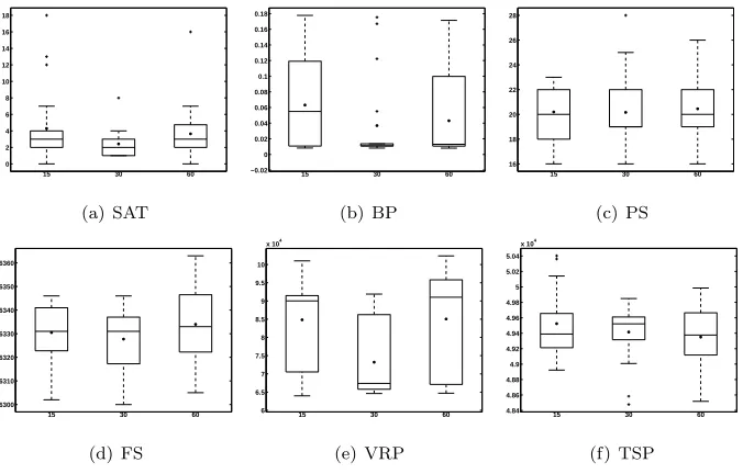
sensitive to the value chosen fortp. In Figure 6 a comparison between the three

values for tp is shown. The asterisk highlights the average performance. A

comparison based on the average values shows that tp = 30 is slightly better

than other values.

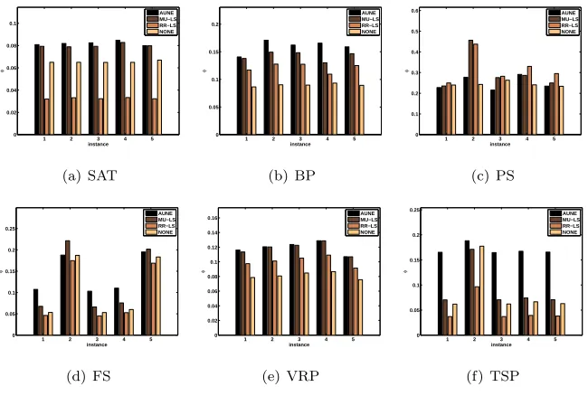
Additionally, to quantify and evaluate the eﬀectiveness of the proposed

noise elimination strategy, we have performed further experiments and

investi-gated into four possible scenarios/strategies for noise elimination: i) Automatic

Noise Elimination (AUNE) (as described in Section 4) ii) No Noise Elimination

(29)

0 2 4 6 8 10 12 14 16 18

15 30 60

(a) SAT −0.02 0 0.02 0.04 0.06 0.08 0.1 0.12 0.14 0.16 0.18

15 30 60

(b) BP 16 18 20 22 24 26 28

15 30 60

(c) PS 6300 6310 6320 6330 6340 6350 6360

15 30 60

(d) FS 6 6.5 7 7.5 8 8.5 9 9.5 10

x 104

15 30 60

(e) VRP 4.84 4.86 4.88 4.9 4.92 4.94 4.96 4.98 5 5.02 5.04 x 104

15 30 60

[image:29.612.138.476.122.338.2]

(f) TSP

Figure 6: Comparing the performance of TeBHA-HH on the ﬁrst instance of various domains for diﬀerent values oftp. The asterisk sign on each box plot is the mean of 31 runs.

in which ruin and recreate and Local Search heuristics only are participated in

tensor construction and iv) MU-LS where mutation and local search heuristics

are considered in tensor construction. Each scenario is tested on all CHeSC

2011 instances and during those experiments tp is ﬁxed as 30 seconds. After

performing the factorization, the ϕ value (Equation 4) is calculated for each

instance at each run. Figure 7 provides the performance comparison of diﬀerent

noise elimination strategies based on theϕvalues averaged over 31 runs for each

instance. It is desirable that theϕvalue, which expresses the model ﬁtness, to

be maximized in these experiments. Apart from the PS and FS domains, our

automatic noise elimination scheme (AUNE) delivers the best ϕ for all other

instances from the rest of the four domains. In three out of ﬁve FS instances,

AUNE performs the best with respect to the model ﬁtness. However, AUNE

seems to be under-performing in the PS domain. The reason for this speciﬁc

case is that the heuristics in this domain are extremely slow and the designated

(30)

of noise properly and consistently. This is also the reason for the almost

ran-dom partitioning of the heuristic space (ﬁgures 5(g), 5(h) and 5(i)). The low

running speed of low level heuristics leads to a low number of collected tensor

frames at the end of the second phase (tensor construction). Without enough

information the factorization method is unable to deliver useful and consistent

partitioning of the heuristic space (like in other domains). That is why, the

histograms belonging to the PS domain in Figure 5 demonstrate a half-half

dis-tribution of heuristics tohN AandhIE heuristic sets. Nevertheless, the overall

results presented in this section supports the necessity of the noise elimination

step and illustrates the success of the proposed simple strategy.

1 2 3 4 5

0 0.02 0.04 0.06 0.08 0.1 instance φ AUNE MU−LS RR−LS NONE (a) SAT

1 2 3 4 5

0 0.05 0.1 0.15 0.2 instance φ AUNE MU−LS RR−LS NONE (b) BP

1 2 3 4 5

0 0.1 0.2 0.3 0.4 0.5 0.6 instance φ AUNE MU−LS RR−LS NONE (c) PS

1 2 3 4 5

0 0.05 0.1 0.15 0.2 0.25 instance φ AUNE MU−LS RR−LS NONE (d) FS

1 2 3 4 5

0 0.02 0.04 0.06 0.08 0.1 0.12 0.14 0.16 instance φ AUNE MU−LS RR−LS NONE (e) VRP

1 2 3 4 5

[image:30.612.145.470.307.526.2]

0 0.05 0.1 0.15 0.2 0.25 instance φ AUNE MU−LS RR−LS NONE (f) TSP

Figure 7: Comparing the model ﬁtness in factorization,ϕ(y axis of each plot), for various noise elimination strategies. Higher ϕvalues are desirable. The x-axis is the ID of each instance from the given CHeSC 2011 domain.

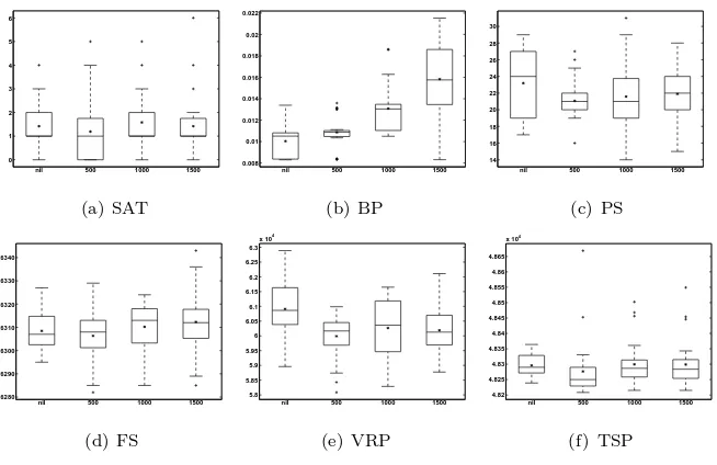
5.3. Switch Time

The value assigned totsdetermines the frequency based on which the

frame-work switches from one acceptance mechanism to another during the search

(31)

been considered in our experiments. For ts = nil, randomly chosen low level

heuristic determines the move acceptance method to be employed at each step.

If the selected heuristic is a member ofhN AorhIE, NA or IE is used for move

acceptance, respectively. The value fortp is ﬁxed at 30 seconds and AUNE is

used for noise elimination during all switch time experiments.

0 1 2 3 4 5 6