http://wrap.warwick.ac.uk/
Original citation:
Rajpoot, K. and Rajpoot, Nasir M. (Nasir Mahmood) (2004) Hyperspectral colon tissue
cell classification. In: SPIE Medical Imaging (MI), US
Permanent WRAP url:
http://wrap.warwick.ac.uk/61376
Copyright and reuse:
The Warwick Research Archive Portal (WRAP) makes this work by researchers of the
University of Warwick available open access under the following conditions. Copyright ©
and all moral rights to the version of the paper presented here belong to the individual
author(s) and/or other copyright owners. To the extent reasonable and practicable the
material made available in WRAP has been checked for eligibility before being made
available.
Copies of full items can be used for personal research or study, educational, or
not-for-profit purposes without prior permission or charge. Provided that the authors, title and
full bibliographic details are credited, a hyperlink and/or URL is given for the original
metadata page and the content is not changed in any way.
A note on versions:
Hyperspectral Colon Tissue Cell Classification
Kashif M. Rajpoot
*a, Nasir M. Rajpoot
†b, Martin J. Turner
‡c aFaculty of Computer Science & Engineering, GIK Institute, Topi Pakistan
bDepartment of Computer Science, University of Warwick, Coventry UK
cFaculty of Computing Sciences & Engineering, De Montfort University, Leicester UK
ABSTRACT
A novel algorithm to discriminate between normal and malignant tissue cells of the human colon is presented. The microscopic level images of human colon tissue cells were acquired using hyperspectral imaging technology at contiguous wavelength intervals of visible light. While hyperspectral imagery data provides a wealth of information, its large size normally means high computational processing complexity. Several methods exist to avoid the so-called curse of dimensionality and hence reduce the computational complexity. In this study, we experimented with Principal Component Analysis (PCA) and two modifications of Independent Component Analysis (ICA). In the first stage of the algorithm, the extracted components are used to separate four constituent parts of the colon tissue: nuclei, cytoplasm, lamina propria, and lumen. The segmentation is performed in an unsupervised fashion using the nearest centroid clustering algorithm. The segmented image is further used, in the second stage of the classification algorithm, to exploit the spatial relationship between the labeled constituent parts. Experimental results using supervised Support Vector Machines (SVM) classification based on multiscale morphological features reveal the discrimination between normal and malignant tissue cells with a reasonable degree of accuracy.
Keywords: Hyperspectral imagery, dimensionality reduction, multiscale morphological features, multiscale
statistical features, SVM classification, colon cell classification
1. INTRODUCTION
The colon is the upper part of the large intestine tube while the rectum is the lower part of this tube. Practically, colon or rectum cancer is characterized as separate cancer instances. Colorectal or bowel cancer is a composite name for colon and rectum cancer. It is the uncontrolled growth of tissue cells in either the colon or rectum which causes the colorectal cancer. According to a recent publication1, over 34,000 new cases of colorectal cancer are diagnosed each year. During the year 2000, there were 16,250 deaths from colorectal cancer in the UK. It is the third most commonly diagnosed cancer in the UK after lung and breast cancer. The UK had one of the worst detection rates for bowel cancer in Europe. Yet 80% of colorectal cancer cases can be treated if caught at an early stage. New improved screening and diagnosis methods could potentially save thousands more lives each year.
High spectral resolution characteristics of hyperspectral sensors preserve important aspects of the spectrum2. Usually, the image data provided by hyperspectral sensors is visualized as a 3D cube because of its intrinsic structure, where the face is a function of spatial coordinates f(x,y) and depth is a function of wavelength d(λ). The image data can also be seen as a stack of multiple 2D images. Each spatial point on the face is characterized by its own spectrum (often called spectral signature). This spectrum is in direct correspondence with the amount of
energy in the material represented, as hyperspectral sensors commonly utilize the simple fact that any body with temperature over absolute zero either emit or reflect the absorbed energy in certain frequency bands. This eventually makes segmentation of different materials possible. Diagnostically important spectral features can be subtle and not easily assessed by the naked eye2. Hyperspectral imaging devices capture such features from the image scene for a deeper understanding and analysis. Having been widely used in remote sensing applications, hyperspectral imaging technology, coupled with microscopy, is now finding a broad set of application areas including biomedicine for disease diagnostics. One such application is the classification of healthy and malignant cells in microscopic level hyperspectral tissue image data. The limited availability of specialist pathological staff and the huge amount of information provided by the hyperspectral sensors means that user fatigue is a significant obstruction in the examination of these images and the identification of colon cancer in early stages.
†
This work deals with the analysis of hyperspectral colon images to classify between normal and malignant tissue sections with a reasonable degree of accuracy and reliable performance. It is an attempt to find a solution which can consistently assist the pathologists. For this work, 12 microscopic level hyperspectral image data cubes of normal and malignant human colon were acquired from archival H & E (hematoxylin & eosin) stained micro-array tissue sections. The resolution of each band is 1024x1024 and 20 bands were used (in order to reduce the computational burden) with wavelengths in the interval 450-650nm.
The reliable detection of malignant cells in stained tissue samples is normally recognized as one of the most demanding and time-consuming tasks in pathology and is a typical example of a pattern recognition problem3. Generally, the task of pattern recognition in images consists of three independent steps, which can be applied to the tissue classification problem as follows: (i) image segmentation: the objects contained in the image scene are
separated from the background. This is the separation of constituent parts of tissue cells, (ii) feature extraction: the
characteristics of each object are quantified. These features, of course, should contain enough discriminant information sufficient to distinguish a normal tissue from a malignant tissue, and (iii) classification: Each object is
assigned to a generic target class. The extracted features from the segmentation labels are utilized to discriminate between normal and malignant tissue cells. In case of classification for hyperspectral images, dimensionality reduction normally precedes the segmentation phase.
In the next section, a brief description of the dimensionality reduction phase is presented. A number of segmentation methods, by exploiting the spatial and/or spectral characteristics, are explained in Section 3. Towards the end, feature extraction schemes using multiscale statistical and morphological features are described, followed by the details of the classification procedure. Finally, we conclude the paper with remarks on segmentation methods and the classification performance, and some future directions.
2. DIMENSIONALITY REDUCTION
Before the formal process of segmentation of hyperspectral imagery, an intermediate step of dimensionality reduction is often involved. Hyperspectral imagery data provides a wealth of information about an image scene which is potentially very helpful in the segmentation of objects. At the same time, the huge size of hyperspectral image data (with tens to hundreds of spectral bands) normally means high computational complexity. High dimensional vector spaces have been found to have some rather unusual and unintuitive characteristics4. This is often recognized as the curse of dimensionality. The goal is to eliminate the redundancy in the data while
simultaneously preserving the discriminant features for segmentation, detection or classification algorithms.
A wide variety of methods can be found in the literature for reducing the dimensionality of a problem. At a higher level, these can be categorized into two groups: (1) linear methods: principal component analysis, factor analysis and
independent component analysis (2) non-linear methods: curvilinear component analysis, curvilinear distance
analysis and multi-dimensional scaling. Other well-known techniques include projection pursuit5 and discrete wavelet transform6. Each of these may have different criteria for projecting the data into lower dimensional spaces (for example: variance in principal component analysis, statistical independence in independent component
analysis, etc.) and thus preferably preserving the dissimilar nature of the characteristics of the data.
In our work, we experimented with principal component analysis (PCA) and independent component analysis (ICA) for reducing the dimension of the image data cubes. The selection was made because of the intrinsic simplicity and well-established mathematical groundings of PCA, and immense potential and capability found in recent years of ICA. There exists a range of ICA modifications, developed largely by the signal processing and machine learning research community, such as FastICA, SparseICA, RADICAL, KernelICA, and FlexICA. In this study, we experimented with the FastICA12 and FlexICA13 variants. The objective of dimensionality reduction here is to reduce the computational complexity as well as to improve the subsequent tasks of segmentation and classification.
2.1. Principal component analysis (PCA)
Principal component analysis (PCA) is a statistical multivariate data analysis tool which attempts to find the natural coordinate axes for the multidimensional dataset. It is the representation of the higher-dimensional data into lower-dimensional orthogonal axes such that it is highly decorrelated. This representation can be considered as the transformation of the original data into a new vector space where the basis vectors are actually a linear combination of the original data vectors.
original data vectors. The amount of variance preserved by the projected data in a certain principal component (eigenvector) direction can be related to the eigenvalue corresponding to that direction.
2.2. Independent component analysis (ICA)
Independent component analysis (ICA) extends the concept of traditional multivariate data analysis techniques (principal component analysis, factor analysis, and projection pursuit) to determine the hidden components in the
data. Unlike PCA, it does not merely attempt to find a decorrelated lower-dimensional representation for the data but also attempts to discover statistically independent components. Although originally developed for blind source
separation tasks in the signal processing area, ICA has recently found applications in diverse areas of multivariate data analysis, dimensionality reduction8, brain imaging9, feature extraction, image classification, and target recognition10. Because of its huge potential, it has been receiving contributions from a broad research community.
In the case of ICA, the data variables are assumed to be a linear mixture of unknown latent variables and the mixing
system is also unknown. Thus the goal is to provide a mathematical estimate for an unmixing matrix. In the following, we formulate the ICA problem in a blind-source separation context and take it further to dimensionality reduction case. Let us assume that the data variabley is made up of a linear combination of the independent latent i
variablesx . Mathematicallyi 11
, for two such variables:
2 22 1 21 2 2 12 1 11 1 x a x a y x a x a y + = + = (1)
where the coefficientsa ’s are unknown. The goal is to estimate these coefficients for the determination ij
ofx and 21 x , giveny and1 y . In matrix notation, the above equation can be written as: 2
AX
Y= (2)
where A is the mixing matrix made up ofaijcoefficients. From the above equation, we know that X can be evaluated
as:
WY
X= (3)
where W is the inverse of the mixing matrix A and is called the unmixing matrix. The above equation is formulated as the ICA model where the objective is to provide an estimate for W such that components in X are maximally independent. In a more elaborative fashion, we can write it as:
− − = − − m m y y y W x x x 2 1 2 1 (4)
where the number of variables inX is dependent on the number of available coefficients in W . In this context, the
utilization of the ICA model for dimensionality reduction is to choose the unmixing matrix W limiting the number ofx components, to say 3 or 4, but in such a way that X contains as much information about the dataY as possible. i
It is the estimation of the unmixing matrixW which creates the main difference between different versions of ICA, which employ different criteria with the unique objective to bring as much information as possible in the extracted individual components. The following sections briefly describe this for FastICA and FlexICA, the subject of our current discussion.
To implement the ICA for multivariate data analysis, we need to satisfy a number of assumptions10: (i). the components should be mutually independent,
(ii). the number of data dimensions (or variables, in other words) must be equal to or greater than the hidden independent components, and
As expressed earlier, ICA can also be seen as an enhancement to PCA and factor analysis (FA). In FA, we assume that the data is of Gaussian nature and the extracted factors need to be merely decorrelated to become independent. In reality, the data often does not follow the Gaussianity restriction. Instead, many real-world datasets have supergaussian or subgaussian density function11. This makes the situation relatively more complex. The ICA proceeds from this stage with the assumption that the data has nonguassian structure. A number of measures can be used to estimate the nongaussianity of the extracted components. Each modification of ICA may employ a different measure for this purpose. This measure is sometimes called a contrast function. The following sections briefly present this for the FastICA and the FlexICA variants.
2.2.1. FastICA
The FastICA12 algorithm utilizes the concepts of entropy and negentropy from information theory to measure the nongaussianity of data variables. By using the maximum entropy approximation for differential entropy, it introduces its own family of contrast functions and explains that it may perform better than the kurtosis contrast function in certain situations. These contrast functions provide a measure of gaussianity and thus, indirectly, a measure for mutual information contained in the components. This assists in extracting components which are as independent as possible. It then uses simple fixed-point algorithms, as compared to gradient-descent methods in conventional estimation approaches, for the optimization of contrast functions in a fast and reliable way. This makes it a computationally highly efficient algorithm.
The above description is not meant to provide a detailed introduction to the FastICA algorithm, but it is rather a bird’s eye view of the method. Further details can be seen in Hyvärinen12.
2.2.2. FlexICA
Most ICA algorithms implicitly assume a particular form for the marginal probability densities of the individual components. On the other hand, FlexICA13 uses generalised exponentials to model the marginal densities enabling it to extract heavy and/or light tailed components. It determines an optimal ICA matrix from the space of decorrelating matrices with the objective of maximizing the likelihood of the data. This is the key to the flexibility of the algorithm to adequately model the marginal densities.
From here, we learn that this algorithm performs particularly well when data has heavy or light tailed density. We also know that kurtosis is a measure of light-/heavy-tailedness of the data density function. Thus the goal here is to utilize and exploit these facts.
2.3. Moving forward
From the above, we notice that ICA is quite sensitive to kurtosis which is a fourth-order statistic. This gives us a clue that we can exploit the ICA procedure by maximizing/minimizing the kurtosis value for the observed data. We employ a simple preprocessing trick to do this in the next section to achieve better performance in segmentation.
At this stage, before proceeding to the next section of segmentation, we must avoid a likely confusion. When we say that the components must have a nonguassian structure, the kurtosis which is a measure of gaussianity (or nongaussianity, in other words) should be associated to these extracted independent components rather than to the original data cube. But we are employing the preprocessing procedure to the original data rather than these components for the maximization of kurtosis statistic value. This is because of the fact that separability of the original data from normal data distribution is actually a measure of separability of extracted components from normal distribution11.
3. SEGMENTATION
After the dimensionality reduction phase, the task ahead is to perform segmentation, the process of dividing the tissue image into cell constituent parts: nuclei, cytoplasm, lamina propria, and lumen. This is an intermediate process performed before the classification which operates on the segmentation labels. We experimented with two slightly different methods of segmenting the hyperspectral image data into its cell-constituent parts, which are: (1) spatial
analysis: by exploiting the spatial relationships between these parts, and (2) spectral analysis: the exploitation of spectral characteristics.
3.1. Spatial analysis: Wavelet based segmentation
In this section, we present an image segmentation algorithm for hyperspectral imagery which is a variation of the conventional wavelet based texture analysis technique. We do not claim it to be the best method for hyperspectral image segmentation but it is quite simple and elegant and has an established foundation. The sole purpose of this practice is to exploit the spatial characteristics in the image rather than the spectral features.
Wavelets are special mathematical functions used to represent a signal/image matched to its resolution and scale. Unlike a conventional Fourier transform, which utilizes sines and cosines of varying amplitude and frequency as its basis functions, the wavelet transform makes use of these scalable wavelet functions. A variety of such functions exists and a well suitable wavelet can be selected specific to an application depending upon the signal/image characteristics to be represented. Wavelet theory is based on strong mathematical foundations and it employs established tools including pyramidal image processing, subband coding, and quadrature mirror filtering. One of the most striking and powerful applications of wavelet theory is the possibility of multiresolution analysis, shown by Mallat in 1987. Multiresolution analysis technique allows us to exploit the signal/image characteristics, matched to a particular scale, which might go undetected in other analysis techniques14. This capability of multiresolution processing paved the way to successful analysis of various kinds of texture.
Scale has been characterized by experts as one of the most important aspect of texture description. Wavelet theory offers intrinsic capability for multiresolutional analysis, and thus provides an opportunity for analyzing a wide variety of textures. A conventional method for wavelet based texture analysis15 is to discard the DC subband (as it often hampers the analysis procedure) and do some kind of preprocessing (low-pass Gaussian, etc.), on rest of the subbands, before constructing the feature images for performing the texture segmentation. In this process, the level of wavelet subband decomposition and the selection of the wavelet filters play a very important role.
Before describing the method, we would like to state what the input to this method is. In the previous section, we have already discussed a couple of dimensionality reduction approaches. This method is linked to the PCA routine for dimensionality reduction. It is not very uncommon in hyperspectral colon tissue imagery to have 80% or even more variance concentrated in the data projected in the first principal component direction (this observation is based on experimental results with image data cubes). Our results (Figure 1) with wavelet based image segmentation method depict that the projected data in the first principal component direction has sufficient spatial information to segment the cell image into constituent parts.
Assuming that each of the constituent parts of the colon tissue cells is a distinct type of texture which may be described by multiresolutional analysis procedure, we experimented with the conventional wavelet based texture analysis technique on this projected data. Results indicated that this is perhaps not a suitable segmentation method for our problem. It led us to make some minor modifications to the above conventional method for achieving reasonable segmentation results. The simple changes made are the use of the DC subband and avoidance of the preprocessing step for the construction of feature images to accomplish the segmentation process.
The rationale behind this change is that the preprocessing stage (smoothing, etc.) in conventional wavelet texture analysis method loses the necessary discriminant information. Also, the discarded DC subband contains important gray value intensity approximation to the original input image. Therefore, inclusion of the DC subband feature image and avoiding the preprocessing stage actually permits the clustering algorithm to observe the intensity variation in the features and assign the labels based on these differences. Although the experimentation with wavelet decomposition level and selection of wavelet filters is not exhaustive, early attempts show that a decomposition level 2 and using daubechies-8 filters perform well for hyperspectral colon tissue segmentation.
3.2. Spectral analysis: ICA based segmentation
An alternative for the segmentation of hyperspectral data is by doing a spectral analysis. This approach is in correspondence with the spectral signature (or spectrum) of each point on the face of the data cube. In practice, we rarely perform a spectral analysis on the original image cube. Rather, we transform it into lower dimensions to remove the spectral redundancy which may hamper the segmentation procedure.
In this section, we describe how statistically independent components extracted through ICA are used for segmentation. We show that improved segmentation results are obtained when FlexICA operation is preceded by high-emphasis filtering as a preprocessing step.
The only a priori information required to extract the independent components, and thus transform the image data cube into lower dimensions, is the number of independent components or regions (or in other words, cell-constituent parts) in the image scene. This is exactly equal to the number of extracted components and it is the new dimension for the transformed image cube. Since a colon cell image consists of four different types of regions, the new dimension of the image cube is 4, reduced from the original depth of 20.
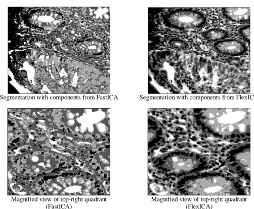
3.2.1. Segmentation without preprocessing
Experimental results, without preprocessing on the original image cube before the ICA operation, using a K-means clustering algorithm on the extracted components are shown (Figure 2). A closer look at the results reveals the under-segmentation artifacts. This may be due to the reason that the components returned by the ICA are not discriminant enough.
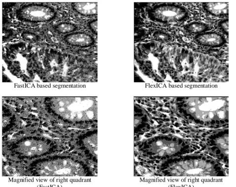
3.2.2. Segmentation with preprocessing
In order to reduce the under-segmentation artifacts seen in Figure 2, a preprocessing operation of high-emphasis filtering is performed on the original hyperspectral image cube before the ICA operation.
As described previously, one of the assumptions to perform ICA on higher-dimensional data is the nongaussianity measure. The fourth-order statistic kurtosis is a classic measure for the quantification of nongaussianity. We also know that the FlexICA algorithm13 is particularly good at separating leptokurtic (supergaussian; heavy-tailed) or
platykurtic (subgaussian; light-tailed) sources. It is also well known that the sample kurtosis is a measure of the heavy- / light-tailedness relative to the normal distribution.
The objective of the preprocessing stage is to bring the distribution of the data to heavy-tailedness. Experiments indicate that the high-emphasis filtering as a preprocessing step forces the distribution towards heavy-tailedness. Figure 4 shows this for the 4-bands of the original image cube. This brings to the front the underlying fact behind the improved segmentation results in the FlexICA case when preceded by the high-emphasis filtering process.
Although the usual purpose of high-emphasis filtering is to restore the edges from a blurred image (image
enhancement), our experiments show that it can be successfully utilized to change the distribution of the data to supergaussian (leptokurtic). There exist a variety of methods in the literature to emphasize the high-frequency details in an image; we adopted the following version:
) , ( ) , ( ) ,
(x y F x y 2F x y
G = −∇ (5)
whereF(x,y)is the original image and∇2F(x,y)is the Laplacian for this image.
Results from Figure 3 also demonstrate that the FlexICA case performs better than the wavelet based segmentation method.
4. CLASSIFICATION
A two-class supervised classification problem is usually formulated in the following way: Given n training pairs )
,
(<xi> yi where <xi>=(xi1,xi2,...,xim) is an input feature vector, andyi∈{−1,+1} is the target label; the task of the discriminant function is to learn the patterns in the training pairs in such a way that, at a later stage, it can predict a reliable yi for a given unknown xi .
The extracted features are fed to a classifier for initial training and later simulation. The classifier used is Support Vector Machines (SVM) for its known advantages16 over the traditional neural networks for many pattern recognition problems. This is particularly the case when the number of features in an input sample vector is very high, which is the situation in our algorithm. The SVM belongs to a large class of learning algorithms called kernel machines which transform input feature space into higher-dimensional space for computational and learning simplicity purposes, such that a relatively optimal decision boundary can be foundyi(WTxi+b)≥1,∀i, where W is
a vector normal to the boundary. This is basically done through the use of a kernel trickK(x,y)=<φ(x),φ(y)>by employing kernel functions (for example: linear, Gaussian, polynomial, etc.), which normally transform the input feature space to a higher-dimensional space for the determination of a linear decision function.
4.1. Feature extraction
The purpose of a feature extraction task in pattern recognition problems is to generate features which can assist in distinguishing between two or more classes. Thus the goal is to extract features which are as discriminant as possible. This surely facilitates the classification procedure. For this purpose, different kinds of features can be exploited. A study of the related literature suggests following different categories: spatial, statistical17, geometrical18, color14, and histogram19 features.
In this study, we experimented with statistical and morphological categories of features. These were extracted at multiple resolutions for the exploitation of both local and global characteristics.
4.1.1. Multiscale features
A close and careful analysis of the problem suggests that the spatial features at a single scale may not suffice for the discrimination between normal and malignant tissue sections, which leads to the investigation of other kind of multiscale features – statistical, morphological, etc. We decided to use multiscale features starting from patch sized 16x16 up to 256x256. This enables us to exploit local as well as global characteristics surrounding a patch at 5-levels for a 16x16 sized patch: 16x16, 32x32, 64x64, 128x128, and 256x256. These multiscale features are concatenated to form a single feature vector corresponding to a 16x16 sized patch. The aim, in both cases, is to extract the best possible information about the location and shape of cell regions in each patch.
4.1.1.1. Statistical features
The shape and location of the regions in a patch can be estimated by descriptive statistics. The statistical tools utilized for this purpose can be divided into three major categories. Each of these may vary regarding their sensitivity to the outliers and asymmetry.
i. Measure of central tendency (location) –
(a) geometric mean
n n i i x / 1
1
∏
= ,(b) harmonic mean
∑
=
n
i xi
n
1
1 / ,
(c) arithmetic mean
∑
= n i i x n 1
1 : these are not robust to outliers
(d) median, and
(e) trimmed mean: both are relatively resistant to the outliers ii. Measure of dispersion (spread) –
(a) standard deviation
1/2 1 2 ) ( 1 1 − −
∑
= n i i xn µ ,
(b) variance
∑
(c) coefficient of variation(σ/µ)*100: these are not robust to outliers, (d) second moment, and
(e) mean absolute deviation
−
∑
=
n
i i x
n 1
1/2 | |
1 µ
: less sensitive to outliers
iii. Measure of normality – kurtosis 4
4 ) (
σ µ −
x E
, skewness 3
3 ) (
σ µ −
x E
These total up to 12 features for a single scale patch. Since features are collected at multiple scales, the feature vector for each 16x16 patch becomes 60-dimensional. These feature vectors are further utilized for training and simulation purposes.
4.1.1.2. Morphological features
The estimation of shape and location of regions in an image can be assisted by the use of morphological features. With regions belonging to normal or malignant cells having specific geometric shapes, the morphological features may prove better than statistical features which are sensitive only to the variability of data values. Out of many available attributes, we opted for nine diverse attributes which are: (i) area: the number of on (with value 1) pixels
in a region, (ii) eccentricity: the eccentricity of the ellipse that has the same second-moment as the region. The
eccentricity is the ratio of the distance between the foci of the ellipse and its major axis length., (iii) equivalent diameter: diameter of a circle with the same area as the region, (iv) Euler number: equal to the number of objects in
the region minus the number of holes in those objects, (v) extent: the proportion of the pixels in the bounding box
that are also in the region, (vi) orientation: the angle (in degrees) between the x-axis and the major axis of the ellipse
that has the same second-moment as the region, (vii) solidity: the proportion of the pixels in the convex hull that are
also in the region, (viii) major axis length: the length (in pixels) of the major axis of the ellipse that has the same
second-moment as the region, and (ix) minor axis length: the length (in pixels) of the minor axis of the ellipse that
has the same second-moment as the region.
We extracted these features for each of the separate labels in a patch. Since there are four labels (constituent parts), each feature vector for a single scale patch becomes 36-dimensional. Thus, the full feature vector containing multiscale morphological features corresponding to a 16x16 sized patch is in 180-dimensions. This is the cause of a huge computational burden for feature extraction and classifier training and/or simulation.
4.2. Classifier training & simulation
After the feature extraction stage, the task ahead is to utilize them in a fruitful way. This section describes the details of the training and simulation of the SVM by the exploitation of these features.
The ICA based technique was performed with the 11 available hyperspectral image cubes to obtain the segmented images, which were further utilized for extracting the features. With an elementary patch of dimensions 16x16 in a 1024x1024 segmented image, the total number of patches sum up to 45,056. We distributed this data into two sets: the training set (size 30,000) and the test set (size 15,056). Both the training and testing data was manually labeled; in order to assist in supervised training as well as to assess the performance of simulation.
We opted for a 3-fold cross validation technique which further divides the training data into 3 sets and uses them iteratively for the selection of favorable parameters for the kernel function. In the beginning, both linear and Gaussian kernel functions were tried but, later on, Gaussian function was chosen because of its superior performance.
5. EXPERIMENTAL RESULTS
This section presents results only for the case when a preprocessing (scaling) step has already been performed on the training and test data. The results given here are the simulation outputs for unknown data, where the size of training or testing data may vary in each case. Given in Table 1 are the comparative results for linear and Gaussian kernel functions. It is worth noting here that both of these results are corresponding to a limited amount of datasets, obtained during the early experimentation phase, and not on the whole 45,056 observations.
Table 2 shows the results for simulation for the same amount of datasets, as for Table 1 [3,000 samples for training, 1,500 for testing], but exploiting the multiscale morphological features this time. Clearly, there is an improvement in classification accuracy and sensitivity. This led us to utilize the morphological features for a comprehensive training of SVM on a large amount of data. Thus we trained SVM with the 3-fold cross validation technique (for a better selection of kernel parameters), employing the Gaussian kernel function, and 30,000 training observations. The final simulation outputs on unknown 15,056 data observations are presented in Table 3.
Table 1: Classifier output with linear & Gaussian kernels (exploitation of multiscale statistical features)
Kernel function Sensitivity Specificity Classification accuracy Gaussian 94% 75% 86%
Linear 85% 65% 77%
Table 2: Results with multiscale morphological features (for limited data)
Sensitivity Specificity Classification Accuracy
99% 74% 89%
Table 3: Final simulation outputs with multiscale morphological features
Sensitivity Specificity Classification Accuracy
89% 85% 87%
Sensitivity is a measure to accurately classify the malignant cell category, whereas the specificity measures the classification accuracy for benign tissues.
6. DISCUSSION & CONCLUSION
As we have stated previously, the wavelet technique is based on spatial pattern recognition, while the ICA method implements spectral pattern recognition. The wavelet based technique is limited as it will produce fine results only when the derived variable covers more than 80% of the data variance. On the other hand, an ICA based approach utilizes all of the extracted independent components and it should be relatively more consistent and reliable than wavelet based technique.
Although we categorized the experimented segmentation techniques as belonging to either spatial or spectral pattern recognition, we do realize that this is not exactly correct. In the wavelet based segmentation case, the input
image is the projected data in the first principal component direction which may retain spectral characteristics. On the other hand, we performed high-emphasis filtering before the ICA operation, which is a kind of spatial processing on the data. Therefore, this categorization merely reflects the apparent exploitation of spatial or spectral characteristics. Both of these can also be jointly described as spatial-spectral analysis methods.
Results demonstrate that morphological features can describe the location and shape of a cellular region better than the statistical case. Two important issues associated with statistical and morphological features, exploited for the tissue cell classification, are:
(i). Although the higher dimensional size of the morphological feature vector is posing extra computational burden, this might be the key for successful classification, as the inherent function of SVM is to transform input feature space to higher-dimensional space to find an optimal decision boundary. Compared with the statistical features case, this is a kind of trade off to achieve improved classification performance.
The segmentation of the constituent parts of cell imagery data works in a completely unsupervised fashion, while the classification of cells from segmentation labels is performed in a supervised way to benefit from human expertise. The overall method can be used without significant human intervention, once the machine is trained on sample data. Although classification performance figures in terms of accuracy, sensitivity, and specificity are promising, a thorough testing of this method on a large data set remains to be investigated. We are also working on improved methods of feature extraction and employing efficient classifiers.
ACKNOWLEDGEMENT
The authors gratefully acknowledge obtaining hyperspectral imagery data used in this work from and having fruitful discussions with Ronald Coifman and Mauro Maggioni of the Applied Mathematics Department of Yale University (USA).
REFERENCES
1. Cancer Research UK, Bowel Cancer Factsheet, May 2002
2. Shaw G., Manolakis D., “Signal Processing for Hyperspectral Image Exploitation,” IEEE Signal Processing Magazine, vol. 19, no. 1, pp. 12-16, Jan. 2002
3. Levenson R., Hoyt C., “Spectral Imaging & Microscopy,” American Laboratory, 2000
4. Jimenez L., Landgrebe D., “Supervised classification in high dimensional space: geometrical, statistical and asymptotical properties of multivariate data,” IEEE Trans. Syst., Man, Cybernet., C, vol. 28, pp. 39-54,
February 1998
5. Jimenez L., Landgrebe D., “High Dimensional Feature Reduction via Projection Pursuit,” Technical Report,
School of Electrical and Computer Engineering, Purdue University, Apr. 1995
6. Bruce L., Koger C., Li J., “Dimensionality Reduction of Hyperspectral Data Using Discrete Wavelet Transform Feature Extraction,” IEEE Trans. Geoscience and Remote Sensing, vol. 40, no. 10, pp. 2331-2338, 2002
7. Davis G., Maggioni M., Coifman R., Rimm D., Levenson R., “Spectral/Spatial Analysis of Colon Carcinoma,”
United States and Canadian Academy of Pathology, Washington DC, Mar 22-28,2003
8. Lennon M., Mercier G., Mouchot M., Hubert-Moy L., “Independent Component Analysis as a tool for the dimensionality reduction and the representation of hyperspectral images,” IGARSS Conference, Sydney, Australia, Jul. 2001
9. Makeig S., Westerfield W., Enghoff, S., Jung. T-P., Townsend J., Courchesne E., and Sejnowski., “Dynamic brain sources of visual evoked responses,” Science, vol. 295, no. 5555, pp. 690-694, Jan. 2002
10. Robila S., Varshney P., “Target Detection in Hyperspectral Images Based on Independent Component Analysis,” SPIE AeroSense, Orlando, FL, Apr. 2002
11. Hyvärinen A., Karhunen J., Oja E., Independent Component Analysis, Chapter 1, Copyright © John Wiley &
Sons, 2001
12. Hyvärinen A., “Fast and Robust Fixed-Point Algorithms for Independent Component Analysis,” IEEE Transactions on Neural Networks, vol. 10, no. 3, pp. 626-634, Apr. 1999
13. Everson R., Roberts S., “Independent Component Analysis: A Flexible Non-linearity and Decorrelating Manifold Approach,” Proceeding of IEEE NNSP98, 1998
14. Gonzalez R., Woods R., Digital Image Processing, Prentice Hall, 2001
15. Rajpoot N., “Texture Classification Using Discriminant Wavelet Packet Subbands,” Proceedings of 45th IEEE Midwest Symposium on Circuits and Systems (MWSCAS'2002) , Tulsa, Oklahoma (USA), Aug. 2002
16. Cristianini N., “Support Vector and Kernel Machines,” 2001, http://www.support-vector.net/tutorial.html 17. Chuai-Aree S., Lursinsap C., Sophasathit P., Siripant S., “Fuzzy C-mean: A Statistical Feature Classification of
Text and Image Segmentation Method,” International Journal of Uncertainty, Fuzziness and Knowledge-Based Systems, vol. 9, no. 6, pp. 661-671, 2001
18. Brunelli R., Poggio T., “Face recognition through geometrical features,” Proceedings of ECCV '92, pp.
792-800, Margherita Ligure, 1992
19. Hetzel G., Leibe B., Levi P., Schiele B., “3D Object Recognition from Range Images using Local Feature Histograms,” Proceedings of CVPR 2001, vol. 2, pp. 394-399, Kauai Island, Hawaii, Dec. 2001
Figures
(Note: There might be some degradation in image display quality due to paper size limitations.)
Colon image spectral band at 460nm Segmentation with conventional wavelet texture analysis approach
Segmentation with modified wavelet based approach
Magnified view of top-right quadrant (wavelet based)
Figure 1: Wavelet based hyperspectral colon tissue image segmentation
Segmentation with components from FastICA Segmentation with components from FlexICA
Magnified view of top-right quadrant (FastICA)
Magnified view of top-right quadrant (FlexICA)
FastICA based segmentation FlexICA based segmentation
Magnified view of right quadrant (FastICA)
Magnified view of right quadrant (FlexICA)
Figure 3: ICA based segmentation with preprocessing by high-emphasis filtering
Distribution plot of 4-bands from the original image cube
Distribution plot of 4-bands from the high-emphasis filtered image
cube
Distribution plot of 4-bands from the high-emphasis filtered image cube (with y-axis scaled between 0 & 100) Figure 4: Distribution plot of image cube bands
Image containing both normal & malignant parts
A benign image (with one misclassified block)
A malignant image (with one misclassified block) Figure 5: Classification results with SVM trained on multiscale morphological features