Model predictive control of forming processes

Faculty of Engineering Technology (CTW)

Model Predictive Control of Forming Processes

Master Thesis

s1116754

B. M.

DE

G

OOIJER

Examination Committee:

prof. dr. ir. A. H.VAN DENBOOGAARD prof. dr. ir. R. AKKERMAN

dr. ir. H. J. M. GEIJSELAERS ir. G. T. HAVINGA

Date:

Model Predictive Control of Forming Processes

Master Thesis

s1116754

B

OUKJE

M

ARIJE DE

G

OOIJER

Institution:

University of Twente

Faculty of Engineering Technology (CTW)

Department of Mechanics of Solids, Surfaces & Systems Chair of Nonlinear Solid Mechanics

Examination committee:

Chair head:prof. dr. ir. A. H.VAN DENBOOGAARD

External member:prof. dr. ir. R. AKKERMAN

Supervisor:dr. ir. H. J. M. GEIJSELAERS

Daily supervisor:ir. G. T. HAVINGA

"Not all who wander are lost"

ABSTRACT

Abstract

Production standards nowadays are continuously increasing. Therefore there is a call for thorough understanding of production processes and new methods of process control. One of these new methods of process control is by making use of a model based control scheme.

The goal of this work is to build a detailed, accurate and fast model of a bending process, which can be used for model-based control.

The bending process of interest is the plastic deformation of a 3 mm steel flap to an angle of 50◦_{. This} flap is part of a demonstrator product especially designed for the MEGaFiT (Manufacturing Error-free Goods at First Time) project in which the University of Twente en Philips cooperate closely.

Finite Element (FE) modeling is used to model the bending process. The output of the FE-model is a force curve similar to the force curve as measured in the bending process.

Proper Orthogonal Decomposition (POD) is used to reduce the result space from a series of FE analysis. Using a Radial Basis Function (RBF) a meta model is fit through this reduced result space. With an average wall time of 0.03 s, the build PODRBF-model is fast enough to be used in an inverse analysis on which a model based control scheme can be designed. The PODRBF-model is detailed and accurate enough to estimate 3 parameters with 10 % accuracy.

PREFACE

Preface

This thesis is written as a completion of the master Applied Mechanics at the University of Twente. When I started my bachelor Advanced Technology five years ago, I never expected to be where I am now. If somebody in high school told me that I would end up doing Mechanical Engineering, I would have laughed at him. However, during my bachelor I found out it were the courses on beam theory and mathematics I enjoyed specifically.

So, in September 2013 I started my master Applied Mechanics. It were the courses on numerical methods, computational optimization and non-linear solid mechanics I liked the most. During my internship in a production facility for diapers I found out another fascination of mine: production processes.

When I sought for a master’s assignment I wanted to combine both interests. In a call with Timo Meinders he convinced me that this assignment wouldn’t be so much programming and I decided to give it a shot. Well, I know better now.

In my first year as a bachelor student my programming skills were those from a student assistant. And by that, I mean that I wasn’t programming myself. Looking back at the past 5 years, and the last 12 months specifically, I can say I have learned a lot. I have grown as a person and I would therefore like to take this opportunity to thank a few people who in some way contributed me in being able to do this.

Jos Havingafor all the input and all the support you gave to me in the past period. No matter how many times I knocked on your door, it was always open.

Haico Steginkfor keeping patient with me. For all the times I was late for dinner and accepting our apartment was probably a little less clean last month. I know it wasn’t easy all the time, but I must say I highly value the advice, time and love you always have for me.

Femke de Gooijerfor being my lovely sister, for all the entertainment you brought to me during our hours in the gym or while having one, or one too many, beers. I really appreciate that you decided to start studying at the University of Twente as well. I am grateful to have you in my life.

Hendrik Spoelhofand the rest of the boys in N242 for all the thesis-related discussions and the less related conversations we had.

I hope one will enjoy reading this thesis as much as I enjoyed writing it.

CONTENTS

Contents

Abstract V

Preface VII

Nomenclature 3

List of Abbreviations 4

1 Introduction 5

1.1 This work . . . 5

1.2 The demonstrator product . . . 5

1.3 Outline of this work . . . 6

2 The production process 7 2.1 The bending module . . . 7

2.2 The bending step . . . 9

3 Modeling the bending step 10 3.1 Software . . . 10

3.2 Geometry . . . 10

3.3 Motion of the punch . . . 12

3.4 Material model . . . 12

3.5 Output of the FE-model . . . 14

4 Parameter study 16 4.1 Parameters incorporated in the FE-model . . . 16

4.2 Variation 1-by-1 . . . 17

4.3 Parameter space . . . 21

5 Approximating the Finite Element Analyses 22 5.1 Proper Orthogonal Decomposition . . . 22

5.2 Radial Basis Function . . . 26

5.3 Force curves using a PODRBF approximation . . . 28

5.4 Variation 1-by-1 using a PODRBF approximation . . . 30

6 Inverse analysis 33 6.1 Weight Function . . . 33

6.2 Error Function . . . 34

6.3 Parameter estimation . . . 36

7 Conclusion 46 8 Discussion & recommendations 47 8.1 Material model . . . 47

8.2 Parameter space . . . 47

8.3 POD basis . . . 47

8.4 Inverse analysis . . . 47

References 48 A Modeling in Marc Mentat 50 A.1 2D model . . . 50

A.2 3D model . . . 50

A.3 Contact modeling . . . 51

CONTENTS

B Parameter study (continued) 53

B.1 All parameters and their values . . . 53 B.2 Force curves for less influential parameters . . . 54

NOMENCLATURE

Nomenclature

A Cross-sectional area [mm2_]

Ajm Amplitude scalar of force curvemcorresponding toj-th POD direction E Young’s modulus [MPa]

F(tn) Force curve discretized inN time steps

L Length [mm]

M Number of force curves in snapshots matrix

N Number of time steps in snapshot matrix

Nϕ Number of POD directions included in the truncated POD basis T Period of the punch motion [s]

¯

Φ Truncated POD basis

¯

A Truncated amplitude matrix

Φ POD basis[Φnj]

ϕ_j Vector containing thej-th POD direction

δpunch Final punch depth [mm]

˙

ε Strain rate [1/s]

γ Spring constant [N/mm]

ˆ

Aj Approximated amplitude scalar corresponding to thej-th POD direction

ˆ

F Vector containing an approximated force curve

ˆ

a Vector collecting the approximated amplitude scalarsAˆj

λ Eigenvalue

A Amplitude matrix[Ajm] F Snapshot matrix[Fnm]

Fm Vector containing force curvem

aj Amplitude vector corresponding to thej-th POD direction am Vector containing the amplitudes corresponding to force curvem

v Eigenvector

z,zm,zp Point in parameter spaceZD_{, indexed withmfor the initial DOE and indexed withpfor}

the validation set

ψ Radial basis function in amplitude approximation

σy Yield stress [MPa] tn Time at pointn[s]

LIST OF ABBREVIATIONS

List of Abbreviations

DOE Design Of Experiments FE(M) Finite Element (Method) LHS Latin Hypercube Sample

1 INTRODUCTION

1

Introduction

Ever increasing production standards demand for advanced methods of process control. Unfortu-nately, variations in process parameters are inevitable and, in the worst case, unmeasurable. These variations can have major influence on the outcome of the final product. Increasing production stan-dards, such as decreasing tolerances and lower scrap rates, therefore call for thorough understanding of production processes and new methods of process control. One of these new methods of process control, is by making use of a model based control scheme.

1.1

This work

In this work the possibility of using model based control in a metal forming process is investigated. The work is done in contribution to the MEGaFiT (Manufacturing Error-free Goods at First Time) project in which the University of Twente and Philips cooperate closely. Within the MEGaFiT project a demonstrator product is designed to study the feasibility of inline process control. The production step of interest is a bending process in which a force curve is measured. Finite Element (FE) analysis will be used to model this production step. The force curves from the finite element analyses are used to gain insight into the influence of (un)measurable parameters. However, as the used FE-model generally takes 1000 seconds to generate a force curve this FE-model is too slow to be used in a control scheme. The 10 most influential parameters are therefore used to build a new, faster model to approximate the force curve. The approximation is based on a Proper Orthogonal Decomposition (POD) combined with Radial Basis Functions (RBF). This PODRBF-model can be used in an inverse analysis on which a control scheme can be based.

The goalof this work is to build a detailed, accurate and fast model of the bending stage, which can be used for model-based control.

1.2

The demonstrator product

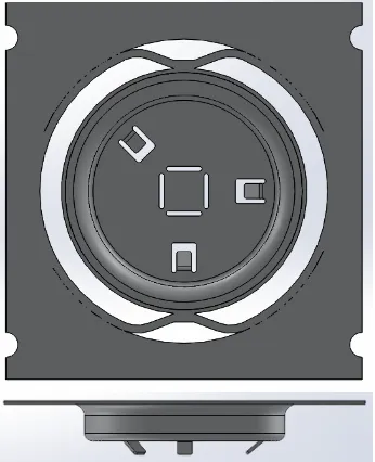
Figure 1.1:Top and side view of the demon-strator product.

A top and side view of the demonstrator product as de-signed for the MEGaFiT project can be found in Figure 1.1. The product is specially designed to study the feasibility of inline process control, therefore there are no specified re-quirements. The three flaps are bend to an angle of 50◦. During this bending step a force curve is measured, as can be found in Figure 1.2a. The three force curves mea-sured upon bending the three flaps differ from flap to flap, as well as per product.

1 INTRODUCTION

Time [s]

-0.3 -0.2 -0.1 0 0.1

Force Y [N]

0 40 80 120 Data1 Data2 Data3

(a)Force curves of the 3 flaps versus production time.

Product no.

30 60 90 120 150

Angle [ ° ] 49 49.5 50 50.5 51

(b)Angles of the rightmost flap versus product number. Figure 1.2:Force curves and angles from 176 demonstrator products as measured in the test setup.

1.3

Outline of this work

zm

FEM

POD

RBF

e(z)

min e(z)

Fexp

z

FFEM(zm)

FFEM(zm)≈ Nϕ

X

j=1

ϕ_j·Ajm

FPODRBF(z) = Nϕ

X

j=1

ϕ_j·Aˆj(z)

e(z) =e(Fexp−FPODRBF(z))

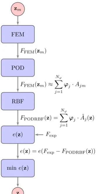
Figure 1.3: Flow diagram to present outline of this work.

The production process of the demonstrator product is described in section 2. How the bending step of in this production process is modeled using finite elements is described in section 3. The main output of the FE-model is a force curve similar to the one as presented in Figure 1.2a.

In Figure 1.3 the further outline of this work is pre-sented. In section 4 it is described how the FE-model is used to do a parameter study. The parameter study is done to find the most influential parameters. By comparing the force curves from the FE-model with the force curves as measured in the test setup the 10 most influential parameters are chosen. Using these 10 most influential parameters a parameter space is defined in which an initial design of experiments is chosen. The sets of input parameters in the initial de-sign of experiments (zm) are used as input for a new

series of finite element simulations.

The force curves from this new series of FE-analyses (FFEM(zm)) are used as input in a Proper Orthogonal

Decomposition (POD). Section 5.1 describes how the force curves are approximated using POD. In section 5.2 it is presented how Radial Basis Function (RBF) are used to go from a discrete input (zm) to a con-tinuous one (z). From this a force curve based on any combination of input parameters (FPODRBF(z)) can be

approximated in a fast way.

Combining this fast approximation with experimental results (Fexp) is the key to an inverse analysis

2 THE PRODUCTION PROCESS

2

The production process

The production process of the demonstrator product is divided in four different modules. Figure 2.1 shows a picture of the production line. The product moves in one long strip through four modules from left to right in the picture. The production speed can range from 12 rpm up to 60 rpm and is the same in each module. In this work the focus is on production with 12 rpm. From the left to the right in Figure 2.1 the modules areCutting,Deep-Drawing,Coiningand lastlyBending. The possibilities in using model-based control are investigated for the bending module. Therefore this section elaborates specifically on that module.

Figure 2.1:Test setup for production of the demonstrator product as used in the MEGaFit project.

2.1

The bending module

The bending module consists of six production steps. A cross-sectional view of the bending module can be found in Figure 2.3. The corresponding demonstrator product in each step can be found in Figure 2.4.

The first step is the entry of the product in the module. In the second step (2.4a, Detail A in Figure 2.3) the three so-called flaps are cut. The rightmost flap is in longitudinal direction, clockwise the next flap is in lateral direction and the last flap is under an angle of 135◦with both other flaps.

Figure 2.2:Picture of the flap as taken in the test setup (Point D in Figure 2.3). After cutting, the flaps are bend to an angle of 50◦_{(2.4b, Detail}

B in Figure 2.3). During this step the bending force of all three flaps is measured. An example of the measured force curves can be found in Figure 1.2a.

After bending the flaps, the flaps are bent back as desired (2.4c, Detail C in Figure 2.3). The extend to which the flaps are bend back can be regulated per product and per flap.

In the last step of the module (2.4d, Point D in Figure 2.3) a picture of the flap in longitudinal direction is captured. From the picture the angle can be calculated with an accuracy of±0.1◦. As processing the image takes some time the information on the final angle of productNis only available when productN+2

2 THE PRODUCTION PROCESS

E

E

A

B

C

E-E

SCALE 1 : 2

D

DETAIL A

SCALE 1 : 1

SCALE 1 : 1

DETAIL B

SCALE 1 : 1

DETAIL C

Figure 2.3:Cross-secional view of the bending module with close-ups of the different production steps.

. (a)Cutting (b)Bending (c)Back bending (d)Angle measurement

. (Detail A) (Detail B) (Detail C) (Point D)

2 THE PRODUCTION PROCESS

A A

SECTION A-A SCALE 1 : 1

punch die flap fixed die gas spring force sensor blankholder Crank drive

AA_doorsnede

A4

SHEET 1 OF 1 SCALE:1:5

DWG NO. TITLE:

REVISION DO NOT SCALE DRAWING

MATERIAL: DATE SIGNATURE NAME DEBUR AND BREAK SHARP EDGES FINISH:

UNLESS OTHERWISE SPECIFIED: DIMENSIONS ARE IN MILLIMETERS SURFACE FINISH: TOLERANCES: LINEAR: ANGULAR: Q.A MFG APPV'D CHK'D DRAWN

Figure 2.5: Cross-sectional view of the bending step with most important parts in-volved.

2.2

The bending step

As the force curve is measured in Detail B in Figure 2.3, this section elaborates on that bending step specifically. The most impor-tant parts involved in the bending step are denoted in Figure 2.5. All parts above the product belong to theupper partof the mod-ule, whereas all the parts below the product belong to thelower partof the module. The upper part of the module is connected to a Bruderer stamping press. The move-ment induces by the stamping press is de-noted with Crank drive in Figure 2.5. The entire upper part moves downwards until the blank holderclamps the product. Thereafter the blank holder guides the further downward movement of the punch. The movement is characterized by a Crank curve as described in more detail in section 3.3. Above the punch a force sensor is placed. This force sensor does not measure negative forces as can be seen clearly in Figure 1.2a.

3 MODELING THE BENDING STEP

3

Modeling the bending step

Probably the hardest part in any finite element analysis is representing the real world in a satisfying way. In this section it is described how the bending step as presented in section 2.2 is modeled using finite elements.

The more elaborated a model becomes, the more expensive. By calling a model expensive one means that it costs a lot of computational power or time to find a solution. The objective is to model the bending step in the cheapest way without compromising too much on the behavior as seen in reality.

A compromise in modeling the real world is already made by focusing only on the third step of the bending module instead of on the total production process. One can imagine that previous production steps can have major influence on the behavior of the product in the bending step. For example deep-drawing can have major influence on the material properties in different directions. However, to lower the computational costs the historical information of the process is completely neglected.

3.1

Software

The bending step is modeled using the FE software MSC Marc 2013.1. A preprocessor called Mentat is used to generate the Marc-input files (.dat). To manage the input and output for the finite element analysis MathWorks’ MATLAB is used. In MATLAB the different input files (.proc) for the preprocessor are generated. The output file generated by Marc (.sts, .t16) are handled in MATLAB as well. The informational flow between the different programs can be found in Figure 3.1. More information on the settings used in Marc Mentat can be found in Appendix A.

MathWorks MATLAB

MSC Marc

Mentat MSC Marc

.proc _.dat

.sts, .t16

Figure 3.1:Information flow between different programs.

3.2

Geometry

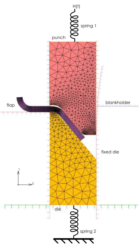
A snapshot of the FE-model with several indicated ‘parts’ can be found in Figure 3.2. The following parts can distinguished:

• flap,

• punch,

• die,

• spring 1 & spring 2,

• crank drive (H(t)),

• blank holder,

• fixed die.

The most important part is theflap. The flap is modeled with 3000 fully integrated bilinear rectangular elements. In the remainder of this work flap and sheet are used interchangeably. The mesh of the flap is finest around the bending area. To decrease numerical noise, no mesh-refinements are done. The material behavior of the flap is modeled using a strain rate dependent material model. The strain rate sensitivity is modeled using a power law as described more elaborately in section 3.4.

3 MODELING THE BENDING STEP

punch

die flap

fixed die

g

blankholder H(t)

gas spring 2 gas spring 1

Figure 3.2:Two-dimensional model in Mentat.

whereas bottom of the die is connected to spring 2. The spring constant (γ) for both springs can be calculated as follows.

γ= AE

L (3.1)

HereinAis the cross-sectional area of the replaced part,Ethe Young’s modulus of the material and

Lthe length of the replaced part.

The punch movement is described by a Crank curve (H(t)). How this movement is implemented in the FE-model is described in section 3.3.

3 MODELING THE BENDING STEP

3.3

Motion of the punch

The motion of the punch is prescribed at the upper node of spring 1 (see Figure 3.2). The travel distance of the punch from its initial position (H(t)in mm) is described by a Crank curve. To set the desired punch depth, the final punch depth (δpunch) is subtracted from the travel distanceH(t).

H(α) =KR·

"

1−cos(α) +1−

p

1−λ2_sin2_(α) λ

#

−δpunch (3.2)

withK= 0.6035a ratio between the two main levers,Rthe eccentric radius (31.45 mm),αthe Crank angle in radians andλ= 0.0850a ratio between the length of the connecting rod and the eccentric radius as provided by Bruderer, the manufacturer of the stamping press.

The travel distance as a function of the Crank angle is rewritten to a function of time. To align the curves at the deepest point ont= 0a shift in Crank angle∆αis introduced.

H(t) =KR·



1−cos _2πt

T −∆α

+

1−q1−λ2_sin2 2πt T −∆α

λ



−δpunch (3.3)

with T the period of the punch motion. The period for a production speed of 12 rpm is 5 s. The resulting punch movement for several punch depths is plotted in Figure 3.3. Note the difference in initial time of contact (t0) due to the different final punch depths.

t0 .

t

-0.3 -0.2 -0.1 0 0.1

H ( t ) -1.5 -1 -0.5 0

δ_{punch= 1}.₅

δ_{punch= 1}.₅₅

δ_{punch= 1}.₆

Figure 3.3:Crank curve for different punch depths (δpunch) and the influence on time of initial contact (t0).

3.4

Material model

The material of the product and thus the flap is AISI420 steel. To model the bending process isotropic material behavior is assumed. This means that the material is assumed to react the same in different directions. As a result the FE-model can be compared to the measured force curves from the test setup of all three flaps.

The flap is deformed plastically. To determine if plastic deformation occurs the Von Mises yield criterion is used.

σy =

q

1

2[(σ11−σ22)2+ (σ22−σ33)2+ (σ33−σ11)2+ 6(σ 2

12+σ223+σ312 )] (3.4)

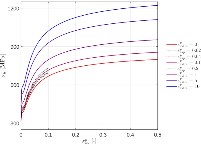
The plastic behavior of the material is modeled using experimental data. The strain rate sensitivity of the material is based on extrapolated data curves [3]. The extrapolated yield-curve for zero strain rate (ε˙p_extra = 0) can be found in Figure 3.4. To model the strain rate dependency a so-called power law is used. This yield-curve at zero strain rateσy(ε|ε˙= 0)is multiplied with an exponential function.

σy(ε,ε˙) =σy(ε|ε˙= 0)·

1 +

_ε˙

10c1

c2

3 MODELING THE BENDING STEP

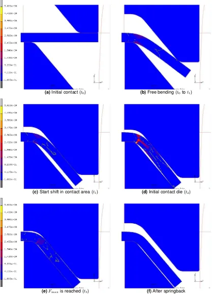
In Figure 3.6 snapshots of the FE-model at various moments in time are displayed. The colors represent the equivalent plastic strain rates. The maximum equivalent strain (εp

eq) and the maximum

equivalent strain rate (ε˙p

eq) reached in the FE-model using nominal settings are slightly over 0.5 and

5/s respectively. The maximum strain rate reached in the experiments (ε˙p

exp) is 0.2/s. The values for

c1and c2used in modeling the bending step are thus strongly extrapolated.

εp_eq [-]

0 0.1 0.2 0.3 0.4 0.5

σy

[M

P

a]

300 600 900 1200

˙

εp_extra= 0

˙

εpexp= 0.02 ˙

εp exp= 0.04 ˙

εp_extra= 0.1

˙

εp exp= 0.2 ˙

εp_extra= 1

˙

εp_extra= 5

˙

εpextra= 10

Figure 3.4:Equivalent plastic strain versus the yield stress for experimental data (ε˙p

exp) and extrapolated data

3 MODELING THE BENDING STEP

3.5

Output of the FE-model

Among other things the output file of the FE-model contains the force each contact body experiences over time as well as the positions of all nodes. MATLAB is used to store both the force curve of interest and the final angle of each simulation.

Force curve

Only the y-component of the force as experienced by the punch is used for further analysis. The force curve from the FE model, as plotted in Figure 3.5, contains a few characteristics.

Att0the punch makes its initial contact with the flap. This initial position of the punch is displayed in

Figure 3.6a. Depending on the final punch depth (δpunch) the time at which this initial contact takes

place can differ (see Figure 3.3). Fromt0tot1the flap is bend without any restrictions, this is called

thefree bendingstage and is displayed in Figure 3.6b.

At t1 there is an abrupt change in slope because the contact area starts to move. This change in

contact area can be seen clearly when comparing Figure 3.6b and Figure 3.6c.

Att2the flap makes contact with the die as displayed in Figure 3.6d. This again causes an abrupt

change in slope. At t = 0the punch reaches is maximum depth. Between t2 andt = 0the flap is

flattened. Within thisflatteningstage the punch experiences its maximum force att3. The FE-model

at maximum force is displayed in Figure 3.6e. The maximum force is not reached when the punch reaches its deepest point due to the strain rate sensitivity of the material.

After the punch reaches its deepest point it starts to move upward. Due to a phenomena called springback the flap moves a bit upward as well. The deformation of the flap after springback can be found in Figure 3.6f.

Time [s]

-0.3 -0.2 0 0.1

Force Y [N]

0 20 40 60 80 100 120

t₀

t₁ t₂ t₃

Figure 3.5:Force curve with different characteristics.

Final angle

3 MODELING THE BENDING STEP

(a)Initial contact (t0) (b)Free bending (t0tot1)

(c)Start shift in contact area (t1) (d)Initial contact die (t2)

(e)Fmaxis reached (t3) (f)After springback

4 PARAMETER STUDY

4

Parameter study

In this section all parameters incorporated in the FE-model are described. By means of a 1-by-1 variation the influence of these parameters is screened. Based on this screening the 1-by-10 most influential parameters are presented in section 4.2. By examining the differences between the FE-model and the experimental data the ranges for some parameters are reduced. Based on the reduced ranges a parameter space is build and presented in section 4.3.

4.1

Parameters incorporated in the FE-model

For convenience the parameters are divided in four groups namely alignment, material, geometric andnumerical. All parameters incorporated in the FE-model and their used values can be found in Appendix B Table B.1. All parameters are varied around a nominal setting.

Alignment parameters

The degrees of freedom with which each part is modeled are depicted in Figure 4.1. The left part of the blank holder is chosen as a reference for thex-alignment. For they-alignment the position of the fixed die is chosen as a reference. The clearance between the punch and the blank holder is chosen to be equal on both sides. The same holds for the clearance between the die and the fixed die. The

x-alignment of the lower part is defined as the difference between the center lines of the punch and the die. An overview of the most important alignment parameters can be found in Table 4.1.

Note that by changing the sheet length and the sheet thickness the mesh of the flap changes as well. The number of elements stays the same, however their width and height changes.

blankholder (right part) blankholder

(left part) punch

die

fixed die (right part) fixed die

(left part)

Figure 4.1:Degrees of freedom for different parts.

Table 4.1:Alignment parameters in FE-model with corresponding minimum, maximum and nominal values.

Alignment parameter min nominal max unit

clearance punch/blankholder (x-alignment) 0 0.0025 0.005 mm clearance die/fixed die (x-alignment) 0 0.002 0.004 mm

x-alignment lower part (die & fixed die) -0.0195 0.0005 0.0205 mm

sheet length (x-alignment cutting) -0.2 0 0.01 mm

sheet thickness (y-alignment upper part) 0.29 0.3 0.31 mm

y-alignment die -0.02 0 0 mm

punch depth (δpunch,y-alignment punch) 1.5 1.56 1.6 mm

blankholder force (y-direction) -50 -300 -500 N

4 PARAMETER STUDY

Material parameters

As only the bottom of the punch is modeled, the removed elasticity is compensated with a spring. The length of the punch head which is modeled (Lhead) is 5 mm. The total length of the punch (Ltot)

as found in the SolidWorks model is 47.3 mm. The Crank drive (Ldrive) is not directly connected to

the top of the punch, but 2 mm below (Figure 2.3). The length of the removed part of the punch can therefore be written as:

L=Ltot−(Lhead+Ldrive) =40.3 mm (4.1)

The cross-sectional area of the punch of 4.97 mm2_{is derived from the SolidWorks model as well. With}

a Young’s Modulus ofE = 210×103_{GPa, the nominal spring stiffness (γ}

1) of the spring connected

to the punch (spring 1) can be calculated using equation 3.1. Hence, the nominal spring stiffness of the punch is 25 898 N/mm.

The nominal spring stiffness (γ2) of the spring connected to the die (spring 2) is calculated in the

same manner. WithLtot = 24.3 mm,Lhead = 5 mm andLdrive= 0 mm, the length of the removed part

of the die isL= 19.3 mm. With a Young’s Modulus ofE= 210 GPa and a cross-sectional area ofA= 4.97 mm2_{, the nominal spring stiffness of the die is calculated to be 54 078 N/mm.}

An overview of the most important material parameters can be found in Table 4.2.

Table 4.2:Material parameters in FE-model with corresponding minimum, maximum and nominal values.

Material parameter min nominal max unit

Poisson ratio 0.29 0.3 0.31

-Young’s modulus (E) 190 210 230 GPa

sheet yield stress premultiplier 0.9 1 1.1 -c1strain rate dependent model 1 1.63 5

-c2strain rate dependent model 0.1 0.44 1

-spring stiffness punch (γ1) 1000 25898 35000 N/mm

spring stiffness die (γ2) 40000 54078 60000 N/mm

friction coefficient 0 0.13 0.2

-Geometric parameters

The fillet radius of the fixed die which is used to smooth the numerical errors in they-component of the contact force, is varied between 10 and 50 mm.

Numerical parameters

The numerical parameters are only varied to find the right settings for the final model in MarcMentat. More on modeling in MarcMentat can be found in Appendix A.

4.2

Variation 1-by-1

All parameters are varied 1-by-1 between their minimum and maximum value to find their influence on the nominal force curve. In a screening all force curves are examined by eye judgment and the 10 most influential parameters are chosen and presented below. Figure 4.3 displays the forces curves based on the 10 most influential parameters, all force curves based on less influential parameters can be found in Appendix B Figure B.1. Based on a comparison with the force curves as measured in the test setup the minimum and maximum values for some parameters are changed.

Clearance die/fixed die

4 PARAMETER STUDY

X-alignment lower part

The x-alignment of the lower part has a large influence on the force curve, specifically in timing. As can be seen in Figure 4.3b a negative misalignment causes the contact area to change earlier. This is due to the fact that with large negative misalignment the punch is in contact with the fixed die. The fixed die forces the punch to the negativex-direction initiating the change in contact area earlier. Both a negative and positive misalignment cause a larger force in the flattening stage with respect to the nominal force curve. The positive misalignment causes the distance with respect to the axis of rotation of the flap to decrease. The negative misalignment has a larger impact on the maximum force than the positive misalignment, due to the contact with the fixed die. The slope after the maximum force is much steeper for negative misalignment, this is due to the friction with the fixed die.

Sheet thickness

The force curves based on changing the sheet thickness in the FE-model are plotted in Figure 4.3c. Generally a larger sheet thickness means a larger force. There is also a slight change in timing due to the change in punch depth. By evaluating the force curves from the test setup (Figure 1.2a) the choice is made to change the minimum and maximum values for the sheet thickness to 0.295 and 0.305 mm respectively.

Y-alignment die

They-alignment of the die has a large influence, specially in timing as can be seen in Figure 4.3d. A negative misalignment causes a different curvature at the start of the free bending stage as there is no contact with the tip of the die initially. The time at which the contact area starts to change and the time at which the contact with the die takes place both shift in positive direction with negative misalignment. Generally a negative alignment means less force needed to bend the flap. In the experimental force curves the peak in the force curve is generally seen wider, than in the FE-model. Therefore the choice is made to set the minimumy-alignment of the die to −0.01 mm.

Punch depth

In Figure 4.3e the influence of changing the punch depth in the FE-model can be found. The most important effect is the change in maximum force. The force curve based on minimum punch depth is not found as such in the force curves from the test setup. Therefore the minimum punch depth is increased to 1.52 mm in the parameter space. The opposite holds for the maximum punch depth, this value is decreased to 1.58 mm. As the punch depth gets smaller, the product is processed in less time. This can be seen clearly in the timing of the force curve. With smaller punch depths the initial contact between the punch and the flap (t0) is later. The initial contact between the die and the flap

becomes later as well. With the minimum punch depth (1.5 mm) the flattening stage is not reached at all, hence there is no contact with the die. A larger punch depth initiates the shift in contact area earlier.

Punch depth [mm]

1.5 1.52 1.54 1.56 1.58 1.6

Angle [

°

]

49.5 50 50.5 51 51.5 52

4 PARAMETER STUDY

To check the numerical noise of the FE-model [8] the final angles corresponding to a wide range of punch depths are plotted in Figure 4.2. The largest angle is established with a punch depth of 1.516 mm. As can be seen in Figure 4.3e this is between the two force curves based on the smallest punch depths. This transition from an increasing final angle to a decreasing final angle has probably to do with the initial contact of the die. For a punch depth of 1.524 mm this stage is entered, whereas with the minimum punch depth this stage is not reached at all.

Sheet yield stress premultiplier

Generally a larger yield stress premultiplier means a larger force as can be seen in Figure 4.3f. Only aftert= 0there is a slight change in timing.

C1strain rate dependent model

In Figure 4.3g the force curves with varied material constant c1can be found. A smaller c1gives a

larger force in all stages. Looking at equation 3.5 a smaller c1means the yield stress becomes higher.

Hence, there is more resistance against deformation. This corresponds with the earlier initiation of the change in contact area for smaller c1. The maximum value for c1is decreased to 3 after examining

various combinations of c1 and c2. Both material parameters are used in the parameter space as

their values are strongly extrapolated from the experimental results.

C2strain rate dependent model

A smaller c2gives a larger force in all stages as can be seen in Figure 4.3h. Again looking at equation

equation 3.5, a smaller c2means a larger yield stress as

lim

c2→0

ε˙

10c1

c2

= 1.

With c2= 0.1 the FEA did not converge. The minimum and maximum values of c2are changed to 0.3

and 0.7 respectively.

Spring stiffness punch

The minimum value used as input for the spring stiffness of the punch is rather low. This is chosen as such to take into account the possible compliance of the machinery. As can be seen in Figure 4.3i a lower spring stiffness produces a wider, but lower peak. As can be seen in Figure 4.3i the force curve based on the maximum spring stiffness (35 000 N/mm) does not differ much from the force curve based on the nominal value for the spring stiffness (25 898 N/mm). Therefore the maximum value for the spring stiffness of the punch is reduced to slightly above the nominal value (26 000 N/mm).

Friction coefficient

4 PARAMETER STUDY

Time [s]

-0.3 -0.2 -0.1 0 0.1

Force Y [N]

0 40 80

120 0_0.001

0.002 0.003 0.004

(a)VAR03 - clearance die/fixed die.

Time [s]

-0.3 -0.2 -0.1 0 0.1

Force Y [N]

0 40 80

120 -0.0195_-0.0095

0.0005 0.0105 0.0205

(b)VAR05 -x-alignment lower part.

Time [s]

-0.3 -0.2 -0.1 0 0.1

Force Y [N]

0 40 80 120 0.29 0.295 0.3 0.305 0.31

(c)VAR10 - sheet thickness.

Time [s]

-0.3 -0.2 -0.1 0 0.1

Force Y [N]

0 40 80 120 -0.02 -0.015 -0.01 -0.005 0

(d)VAR11 -y-alignment die.

Time [s]

-0.3 -0.2 -0.1 0 0.1

Force Y [N]

0 40 80

120 1.5_1.524

1.548 1.572 1.6

(e)VAR12 - punch depth.

Time [s]

-0.3 -0.2 -0.1 0 0.1

Force Y [N]

0 40 80

120 0.9_0.95

1 1.05 1.1

(f)VAR22 - sheet yield stress premultiplier.

Time [s]

-0.3 -0.2 -0.1 0 0.1

Force Y [N]

0 40 80 120 1 1.63 2.5 3.6 5

(g)VAR23 - c1.

Time [s]

-0.3 -0.2 -0.1 0 0.1

Force Y [N]

0 40 80 120 0.1 0.25 0.43767 0.75 1

(h)VAR24 - c2.

4 PARAMETER STUDY

Time [s]

-0.3 -0.2 -0.1 0 0.1

Force Y [N]

0 40 80

120 1000₁₀₀₀₀

18000 25898 35000

(i)VAR27 - spring stiffness punch

Time [s]

-0.3 -0.2 -0.1 0 0.1

Force Y [N]

0 40 80

120 0_0.05

0.1 0.13 0.2

(j)VAR29 - friction coefficient Figure 4.3:FEM curves for most influential parameters (cont.).

4.3

Parameter space

The 10 most influential parameters from the screening described in the previous section are used to define a parameters space (ZD). In Table 4.3 an overview is given from the new minimum and maximum values based on the screening. These minimum and maximum values are the minima and maxima of the real interval (Z(d)) on which each parameter (z(d)_{) is defined. Hence,D = 10, and a}

point in the parameter space can be defined as:

z={z(1), z(2),· · ·, z(10)} ∈ZD (4.2)

Comparing Table B.1 and Table 4.3 one can see that by means of the screening the variables in the FE-model are reduced from 23 to 10. Only the alignment and material parameters are used in the parameter space.

Using a Latin Hypercube Sample (LHS), 4960 points in the parameter space were generated as an initial Design Of Experiments (DOE). Each point from the initial DOE (zm) is used as input for a new set of finite element analyses.

Table 4.3:Minimum and maximum values for selected variables used to define the parameter space.

Variable Description min(Z(d)_{) max(Z}(d)_{) unit}

Alignment

z(1)= VAR01 clearance die/fixed die 0 0.004 mm

z(2)_{= VAR05 x-alignment lower part (die & fixed die) -0.0195 0.0205 mm}

z(3)_{= VAR10 sheet thickness 0.295 0.305 mm}

z(4)= VAR11 y-alignment die -0.01 0 mm

z(5)_{= VAR12 punch depth 1.52 1.58 mm}

Material

z(6)_{= VAR22 sheet yield stress premultiplier 0.9 1.1} -z(7)_{= VAR23 c}

1strain rate dependent model 1 3

-z(8)_{= VAR24 c}

2strain rate dependent model 0.3 0.7

-z(9)_{= VAR27 spring stiffness punch 1000 26000 N/mm}

-5 APPROXIMATING THE FINITE ELEMENT ANALYSES

5

Approximating the Finite Element Analyses

It takes approximately 15 minutes for the FE-model to generate a solution. As production speeds range between 12 to 60 rpm the FE-model is too slow for use in a control algorithm. In this chapter a fast and accurate substitute for the FE analysis is sought. The objective is to reduce the result space using a Proper Orthoghonal Decomposition (section 5.1). Thereafter a meta model based on the input parameters is fitted through the reduced result space using Radial Basis Functions (section 5.2).

5.1

Proper Orthogonal Decomposition

Proper Orthogonal Decomposition (POD) is a method which enables to build a low dimensional approximation of a high dimensional problem. In this section POD is used to approximate the results of a finite element analysis.

Each point in the parameter space from the initial DOE (zm) defined in section 4.3 is used as input for a finite element analysis. In total 4960 simulations were done. Seven simulations failed, therefore 4953 complete force curves were generated.

The FE analyses were done using a variable time step. The average amount of steps needed was 290, whereas the minimum was 228 and the maximum was 552. To be able to compare the force curves each curve is interpolated in exactlyN = 200time steps (F(tn)). Note that by interpolating

with less time steps than in the original simulation the force curve is slightly smoothed. The force sensors in the production line as presented in section 2.2 do not measure negative forces. This can be seen clearly in the experimental force curve in Figure 1.2a. This is incorporated in the approxima-tion by setting all negative forces equal to 0. These force curves are calledsnapshotsin POD jargon [1]. The collection ofM snapshots can be stored in a so-called snapshot matrix (F). So, Fis anN

byM matrix containing theM = 4953force curves generated using the FE-model, inN = 200time steps.

F= [Fnm] = [Fm(tn)] with n= 1..N

m= 1..M (5.1)

=



 

F1(t1) · · · FM(t1)

..

. . .. ...

F1(tN) · · · FM(tN)



 

To explain the principle of proper orthogonal decomposition an example with N = 2 results per snapshot andM = 3snapshots is given. Consider 3 force curves at time steptnandtn+1. Normally

these would be represented as in Figure 5.1a. However, the snapshot matrix can be considered as a set ofM, N-dimensional vectors as well [1]. These three vectors are normalized and plotted in Figure 5.1b.

Instead of looking at the force curves in the current basis, a new basis is sought as such that the pro-jection of all force curves is maximum. This new basis is called the POD basis (Φ) and is, depending on the dimensions of the snapshot matrix, anN ×M orN×N matrix. In this workN < Mand the POD directions are just the eigenvectors (vj) of the matrixC=F·FT _[2].

ϕ_j =vj with j= 1..N (5.2)

The total POD basis can be built by storing the POD directions in descending order of corresponding eigenvalues [1]. The POD directions have sizeN×1. Hence, by storing theN POD directions the total POD basis has sizeN×N.

Φ= [ϕ₁ · · ·ϕ_j · · · ϕ_N] (5.3) All force curves in the snapshot matrix can be obtained by multiplying the POD basis with a so-called amplitude matrixA.

5 APPROXIMATING THE FINITE ELEMENT ANALYSES

Fm

101 103 105 107 109

tn tn+1

F₁

F₂

F₃

(a)Snapshot of 3 force curves attnandtn+1.

Fm(tn)

-0.6 -0.4 -0.2 0 0.2 0.4 0.6

Fm

(

tn+

1

)

0 0.2 0.4 0.6

F1/|F1|

F2/|F2|

F3/|F3|

ϕ1

ϕ2

(b)Force curves represented asM = 3,N = 2-dimensional vectors with corresponding POD basis.

Figure 5.1:Two different representations of a force curve.

As the POD basis is orthogonal it holds thatΦT ·Φ=Iand the amplitude matrix can be calculated easily.

A=ΦT ·F (5.5)

Force curve in the POD basis

A single force curveFmcan be obtained by multiplying the POD basis with a corresponding ampli-tude vectoram. This amplitude vector is them-th column of the amplitude matrix and contains all

amplitudes corresponding to thej-th POD direction of force curve Fm. Note that this can also be

written as the multiplication of a POD direction (ϕ_j) with its corresponding amplitude scalar (Ajm)

and summing over the number of POD directions (N).

Fm=Φ·am

=

N

X

j=1

ϕ_j·Ajm

(5.6)

Coming back to the example with the three force curves at timestnandtn+1. The first POD direction

5 APPROXIMATING THE FINITE ELEMENT ANALYSES

vectors representing the force curve. So, apparently not all POD directions are needed to represent the force curves. By using the first POD direction only, one can already get a good representation of a force curve. Hence, the force curves in the snapshot matrix can be approximated in a lower dimension by truncating the POD basis and amplitude matrix. The number of POD directions in the truncated POD basis (Nϕ) is not established.

F≈Φ¯ ·A¯ (5.7)

where,

¯

Φ= [Φnj],A¯ = [Ajm] withj= 1..Nϕ< N m= 1..M

n= 1..N

In the approximation of the FE model the principle is the same, onlyN = 200 andM = 4953. The number of POD directions needed in the truncated POD basis (Nϕ) to capture the behavior as seen

in Figure 4.3 is not known yet. In Figure 5.2 the first four normalized POD directions are plotted. One can see that the first POD direction looks very much like the force curve in Figure 3.5.

t

-0.3 -0.2 -0.1 0 0.1

ϕ

/

m

a

x

|

ϕ

|

Figure 5.2:First 4 POD directions.

To find out how many POD directions are needed to represent the force curve the Root Mean Square Error (RMSE) is introduced. The RMSE is a measure for the difference between the force curve from the finite element analysis and the force curve in the truncated POD basis. The difference between the two force curves is squared and averaged over the number of time steps (N). Subsequently the square root is taken. Note that an interpolated force curves from the FE model can be written directly in the POD basis by combining equation 5.4 and 5.4.

FPOD = ¯Φ·Φ¯

T

·F (5.8)

And the RMSE can be defined as:

RMSE(zm, Nϕ) =

v u u t 1 N N X n=1

FFEM(tn,zm)−FPOD(tn,zm, Nϕ)

2

(5.9)

where

FFEM(tn,zm) =Fm

FPOD(tn,zm, Nϕ) = ¯Φ·Φ¯ T

5 APPROXIMATING THE FINITE ELEMENT ANALYSES

Note that every force curve can thus be split in a part within the POD basis and a part outside the POD basis. Recall that in this workN < M and the original POD basis had sizeN×N.

F(tn) =





Nϕ

X

j=1

Φnj·ΦTnj



·F(tn) +





N

X

j=Nϕ+1

Φnj·ΦTnj



·F(tn) (5.10)

The error due to truncation of the POD basis can thus be defined as:

¯

e(tn) =





N

X

j=Nϕ+1

Φnj·ΦTnj



·F(tn) (5.11)

Which is the same asFFEM(tn)−FPOD(tn, Nϕ), the error in equation 5.9. For every point in the

parameter space zm the root mean square error is calculated using a different number of POD-directions. The average root mean square error (RMSE) over all force curvesM is calculated and plotted in Figure 5.3.

RMSE(Nϕ) =

1

M M

X

m=1

RMSE(zm, Nϕ)

Theoretically the average root mean square error due to truncation should be 0 whenNϕ =N. At Nϕ≈170the average root mean square error drops to the computational error and could therefore

not be calculated.

N

0 20 40 60 80 100 120 140 160 180

_____

RMSE [N]

10-6 10-4 10-2 100

5 APPROXIMATING THE FINITE ELEMENT ANALYSES

5.2

Radial Basis Function

With the truncated amplitude matrix the force curves can only be obtained for the set of input param-eters (zm). So, now the goal is to approximate the force curve for any set of parametersz, instead of

one of the sets of input parameters.

ˆ

F(z) = ¯Φ·aˆ(z) (5.12)

Hence, a function should be found to predict the amplitude vector for any set of parameters aˆ(z). This is done by interpolating the set of known amplitudes for each POD direction throughout the parameter space. Hence, each row of the amplitude matrix (aj) is interpolated in ZD. To do this,

Radial Basis Functions (RBF) are chosen as an interpolation method.

It is assumed that the amplitude scalarAˆj(z)for everyj-th POD direction can be written as the linear

combination of a weight (wk) and a radial basis function (ψ) [4]. This RBF is some function based of

the euclidean distance between the argument (z) and the known points in the parameter space (zk).

ˆ

Aj(z) = M

X

k=1

wk·ψ(zk−z) (5.13)

By evaluating the amplitude scalar Aˆj(z)on the known points in the parameter space (zm) the

un-known weights can be found.

Ajm= ˆAj(zm) (5.14)

Doing this for all points in the parameter space gives:

aj =

M

X

k=1

wk·ψ(zk−zm)

=

M

X

k=1

wk·Ψkm=w·Ψ

(5.15)

Leading to:

w=aj·Ψ−1 (5.16)

Where wis the1×M vector containing the weights for allM basis functions and Ψis the matrix containing the radial basis functions evaluated at allM points. Substituting equation 5.16 into equa-tion 5.13 gives an expression for the amplitude scalar for thej-th POD direction for any set of input parameters:

ˆ

Aj(z) =aj·Ψ−1·ψ(zk−z) (5.17)

Now the function to predict the amplitude vectoraˆ(z)can be defined as the vector collecting theNϕ

approximated amplitude scalars.

ˆ

a(z) = ˆAj(z) with j = 1..Nϕ (5.18)

The above-mentioned generally holds for all types of radial basis functions. In this work the choice is made to use a multiquadric radial basis function with scaling in each dimension.

ψ(zk−z) =

q

c2

k+||θ◦(zk−z)||2 (5.19)

hereinck is a local shape parameter andθa global scaling parameter [4]. The global scaling

param-eterθscales the parameter space in each dimension as follows.

||θ◦(zk−z)||=

v u u t D X d=1 θd

z(_kd)−z(_kd) 2

5 APPROXIMATING THE FINITE ELEMENT ANALYSES

The values forθ can either be fixed or optimized per dimension. Whenθ is chosen to be same in each dimension a value ofθd=

D

√

M is suitable when using a normalizedz. The optimization ofθis done by means of a Leave One Out Cross-Validation (LOOCV). The cross-validation valuesmcan

be found easily. By minimizing the euclidean norm ofmthe optimal values forθcan be found [4]. m= ˆA

(−m)

j (zm)−Ajm= wk

(Ψ−1₎ kk

(5.21)

The local shape parametersck can be fixed or scaled to their nearest neighbor. Whenckis scaled to

its nearest neighbor the values forck can be calculated as follows [4]. ck =

mink6=m||θ◦(zk−zm)||

maxmcm

(5.22)

The influence of changing both parameters in the multiquadric radial basis function can be found in Figure 5.4. As one can see in Figure 5.4a changingck andθhas the opposite effect. Loweringck

gives a steeper radial basis function, whereas increasingθgives a steeper function. In Figure 5.4b the result of changingck andθin an interpolation can be found. The red line is an interpolation with ckconstant, and highθ. This leads to a steep function in the area with few data points (z=−4..−1).

The blue line is an interpolation withck constant, and lowθ. This gives large oscilations in area with

many data pionts (z=−1..0). In black the interpolation function withckscaled to its nearest neighbor

is plotted. One can see that this interpolation fits the data points nicely in both the area with few data points as the area with many data points.

||zk−z||

-1 -0.5 0 0.5 1

ψ 0 0.2 0.4 0.6 0.8 1 1.2

ck= 0.5 ck= 0.1

ck= 0.01

||zk−z||

-1 -0.5 0 0.5 1

ψ 1 1.05 1.1 1.15 1.2

θ= 0.5 θ= 0.1 θ= 0.01

(a) Multiquadric radial basis function (ψ). On the left: varying the shape parameter (ck) and fixed scaling (θ= 1) . On the right: fixed shape parameter (ck= 1) and varied scaling (θ).

−4 −2 0

−2 −1 0 z ˆ a ( z )

(b)Interpolation using a radial basis function with:ckfixed and highθ(red),ckfixed and lowθ(blue) andckscaled to the nearest neighbor (black).

5 APPROXIMATING THE FINITE ELEMENT ANALYSES

5.3

Force curves using a PODRBF approximation

Now a force curve based on any point in the parameter spacezcan be approximated using PODRBF as follows.

FPODRBF(tn,z, Nϕ) = ¯Φ·aˆ(z)

=

Nϕ

X

j=1

ϕj·Aˆj(z)

(5.23)

The radial basis functions are scaled to their nearest neighbor (ck) and fitted using a fixed scaling

of θ = 10√₅₀₀₀

≈2.3for the first 184 POD directions and an optimized scaling for the first 25 POD directions. To test the quality of both PODRBF-models extra points in the parameter space are generated. This is done by calculating the minimum Euclidean distance between a new LHS of 1000 points and the original DOE. The 100 pointspwith maximum Euclidean distance with respect to the original DOE are chosen as a validation set.

So, to recapitulate there are 5 types of force curves:

• FFEM(t), a force curve from the FE-model.

• FFEM(tn), a force curve from the FE-model discretized inN time steps.

• FPOD(tn, Nϕ), a force curve from the FE-model projected in the truncated POD basis. • FPODRBF(tn, Nϕ), a force curve approximated using radial basis functions with fixed scaling. • FPODRBF(tn, Nϕ, θopt), a force curve approximated using radial basis function with optimized

scaling.

The force curves from the FE-model are based on points in the parameter space from either the original DOE (zm) or the validation set (zp, withp= 1..100). The PODRBF approximation is defined throughout the whole parameter space (ZD_{) and can therefore be based on any point (z).}

In Figure 5.5a different types of force curves based on a point from the validation set are plotted (zp). One can see that the force curve plotted directly from the FE-model shows peaks in the free bending stage. This high frequent behavior is due to numerical noise. The force curve from the FE-model is projected in a truncated POD basis withNϕ = 5. With this few POD directions the sudden

change in slope initiated by the change in contact area (see Figure 3.5) is captured poorly. The PODRBF approximation with fixed scaling and Nϕ = 184 overestimates the force curve, specially

around the maximum force. However, the approximation does capture the sudden change in slope. An approximation with this many POD directions starts to show high frequent behavior. The PODRBF approximation with optimized scaling andNϕ= 5is almost identical to the original force curve written

in the POD basis.

Time [ms]

-0.3 -0.2 -0.1 0 0.1

Force Y [N]

0 20 40

FFEM(t)

FPOD(tn, Nϕ= 5)

FPODRBF(tn, Nϕ= 184)

FPODRBF(tn,θopt, Nϕ= 5)

(a)Force curve from the FE-model, written in the POD basis and using a PODRBF approximation with fixed scaling and optimized scaling.

tn

-0.3 -0.2 -0.1 0 0.1

| E ( tn ) | [N ] 10-4 10-2 100

(b) Absolute error per time step of the interpolated force curve from the FE-model compared to the POD basis, the PODRBF approximation with fixed and op-timized scaling.

5 APPROXIMATING THE FINITE ELEMENT ANALYSES

Table 5.1:Amplitudes corresponding to the first 5 POD directions of the force curves in Figure 5.5a.

ϕ₁ ϕ₂ ϕ₃ ϕ₄ ϕ₅

APOD 267.43 -25.97 -64.76 -6.71 16.47 APODRBF 303.17 -40.04 -63.59 -5.25 3.18 APODRBF(θopt) 269.90 -27.98 -64.19 -5.57 14.18

In Figure 5.5b the absolute error between the interpolated curve from the FE-model and the different approximations is plotted.

|E(tn)|=

FFEM(tn,zp)−Fapprox(tn,zp)

(5.24)

The curve of the absolute error of the PODRBF approximation using optimized scaling (in red) is very similar to the absolute error of the force curve written in the POD basis withNϕ= 5(in gray). Only

aroundt= 0the absolute errors differ slightly. The absolute error of the PODRBF approximation with fixed scaling looks completely different from the two other curves (in blue).

In Table 5.1 the amplitudes corresponding to the first 5 POD directions are given. As expected from Figure 5.5 the amplitudes of the force curve projected in the POD basis and the PODRBF approximation with optimized scaling are alike. The PODRBF approximation with fixed scaling show large deviations from the correct amplitudes.

The average root mean square error between FFEM and FPODRBF over the total validation set is

calculated (see equation 5.9) and plotted in Figure 5.6.

RMSE(Nϕ) =

1

P P

X

p=1

RMSE(zp, Nϕ) (5.25)

However, the RMSE between the force curve from the FE-model projected in the POD basis withNϕ

POD-directions (FPOD) and the PODRBF approximation (FPODRBF) can be calculated as well.

RMSE(zp, Nϕ) =

v u u t 1 N N X n=1

FPOD(tn,zp, Nϕ)−FPODRBF(tn,zp, Nϕ)

2

(5.26)

where

FPOD(tn,zp, Nϕ) = ¯Φ·Φ¯ T

·Fp

FPODRBF(tn,zp, Nϕ) = ¯Φ·aˆ(zp)

Leading to:

RMSE(zp, Nϕ) =

v u u t 1 N N X n=1 ¯

Φ·_Φ¯T_{·Fp−ˆa(zp)}2 _(5.27)

The latter RMSE gives an indication of how well the RBF predicts the amplitudes and thus the force curve. Both RMSE’s are plotted in Figure 5.6. As one can see the RMSE between FFEM and FPODRBF using fixed scaling (in blue) does not become smaller than 2 N. By increasing the

num-ber of used POD directions to 20, the error betweenFFEM and FPODRBF is the same as the error

betweenFPOD andFPODRBF. So, adding an extra POD direction does not add any accuracy to the

approximation.

By using a radial basis function with optimized scaling (in red) the RMSE betweenFFEMandFPODRBF

5 APPROXIMATING THE FINITE ELEMENT ANALYSES

0 5 10 15 20 25 30 35 40

100 101

Nϕ

_____ RMSE [N]

Fixed scaling, F FEM Fixed scaling, F

POD Optimized scaling, F

FEM Optimized scaling, F

POD

Figure 5.6:Average root mean squared error of the test setzpversus the number of used POD directions (Nϕ) with fixed scaling of 10√

5000and optimized scaling for the first 25 POD directions. RMSE betweenFFEM and

FPODRBFis plotted with a circle, RMSE betweenFPODwithNϕPOD-directions andFPODRBFis plotted with a

+-sign.

5.4

Variation 1-by-1 using a PODRBF approximation

Now all parameters are varied 1-by-1 in the PODRBF approximation with optimized scaling and

Nϕ = 25to reproduce Figure 4.3. Note that in the remainder of this work those settings are used to

approximate a force curve. So,

FPODRBF(tn,z) =FPODRBF(tn, Nϕ= 25θopt)

is evaluated using nominal settings (z0) and varying one parameter (z(d)_{) at a time. Note that these}

points (z) are not used to make the POD basis. For comparison the force curves from the FE-model at minimum and maximum values are plotted as well.

When comparing all plots in Figure 5.7 it can be seen that generally the force curves from the PODRBF-model are smoother than the curves from the FE-model. Abrupt changes in slope are not captured by the PODRBF-model. For example the slope of the curve upon initial contact is in most cases not as steep as in the FE-results. However, generally the characteristics in force curve each parameter causes are captured adequately.

Clearance die/fixed die

In Figure 5.7a one can see that the influence of the clearance is slightly overestimated by the PODRBF-model, the force curves lay above the curves of the FE-model.

X-alignment lower part

The alignment inx-direction of the lower part has a large influence on the timing of the force curve. The PODRBF approximation captures this behavior reasonably good as can be seen in Figure 5.7b. Remember that the POD basis was built without any negative forces (section 5.1). Strikingly the force curves from the PODRBF-model do drop to negative values.

Sheet thickness

In Figure 5.7c one can see that the influence of the sheet thickness is slightly underestimated by the PODRBF model. The shift in initial contact between punch and flap (t0) is captured only after the

initial contact took place.

Y-alignment die

5 APPROXIMATING THE FINITE ELEMENT ANALYSES

Punch depth

Upon initial contact the PODRBF approximation falls below zero for small punch depths as can be seen in Figure 5.7e. However all shifts in timing are precisely captured by the approximation.

Sheet yield stress premultiplier

In Figure 5.7f the force curves with varying sheet yield stress premultiplier are plotted. The peak in the force curve is somewhat more flat for a yield stress multiplier smaller than 1.

C1 strain rate dependent model

The influence of the material constant c1 from the strain rate dependent model is captured pretty

good as can be seen in Figure 5.7g. Around the maximum force the influence of c1is slightly

under-estimated.

C2 strain rate dependent model

As for c1, the influence of c2is underestimated around the maximum force as well. The force curves

with varying c2can be found in Figure 5.7h.

Spring stiffness punch

In Figure 5.7i the force curves with varying spring stiffness of the punch are plotted. The influence of a low spring stiffness is overestimated, whereas the influence of a high spring stiffness is underesti-mated. The force curve from the PODRBF-model forγ= 1000is, in contrast to all other curves, less smooth than the curve from the FE-model.

Friction coefficient

Figure 5.7j displays the force curves from various friction coefficients. Compared to Figure 4.3j the influence of varying the friction coefficient seems to increased. However, note that in the PODRBF-model all friction coefficients are changed at once.

Time [s]

-0.3 -0.2 -0.1 0 0.1

Force Y [N]

-20 0 20 40 60 80 100 120 140

0 0.001 0.002 0.003 0.004

(a)z(1)_{- clearance die/fixed die}

Time [s]

-0.3 -0.2 -0.1 0 0.1

Force Y [N]

-20 0 20 40 60 80 100 120 140

-0.02 -0.01 0 0.01 0.02

(b)z(2)_{-x-alignment lower part.}

5 APPROXIMATING THE FINITE ELEMENT ANALYSES

Time [s]

-0.3 -0.2 -0.1 0 0.1

Force Y [N]

-20 0 20 40 60 80 100 120 140 0.295 0.2975 0.3 0.3025 0.305

(c)z(3)_{- sheet thickness.}

Time [s]

-0.3 -0.2 -0.1 0 0.1

Force Y [N]

-20 0 20 40 60 80 100 120 140 -0.01 -0.0075 -0.005 -0.0025 0

(d)z(4)_{-y-alignment die.}

Time [s]

-0.3 -0.2 -0.1 0 0.1

Force Y [N]

-20 0 20 40 60 80 100 120 140 1.52 1.535 1.55 1.565 1.58

(e)z(5)_{- punch depth.}

Time [s]

-0.3 -0.2 -0.1 0 0.1

Force Y [N]

-20 0 20 40 60 80 100 120 140 0.9 0.95 1 1.05 1.1

(f)z(6)_{- sheet yield stress multiplier.}

Time [s]

-0.3 -0.2 -0.1 0 0.1

Force Y [N]

-20 0 20 40 60 80 100 120 140 1 1.5 2 2.5 3

(g)z(7)- c1(log(ε˙0)).

Time [s]

-0.3 -0.2 -0.1 0 0.1

Force Y [N]

-20 0 20 40 60 80 100 120 140 0.3 0.4 0.5 0.6 0.7

(h)z(8)- c2(z).

Time [s]

-0.3 -0.2 -0.1 0 0.1

Force Y [N]

-20 0 20 40 60 80 100 120 140 1000 7250 13500 19750 26000

(i)z(9)- spring stiffness punch.

Time [s]

-0.3 -0.2 -0.1 0 0.1

Force Y [N]

-20 0 20 40 60 80 100 120 140 0 0.05 0.1 0.15 0.2

(j)z(10)- friction coefficient.