Model Selection

Model Selection

Arturo Perez Adroher

Author: Arturo Perez Adroher

Supervisor (Rabobank): Pavel Mironchyck

Supervisor (Rabobank): Viktor Tchistiakov

Supervisor (UTwente): Berend Roorda

Abstract

This thesis is on the comparison of model selection algorithms. It builds a framework for relevant algorithms or criteria that have been proposed so far in literature and that lead to a model easy on interpretation and with high predictive power. The properties and performance of these model selection algorithms are studied and compared.

We further propose redeveloped algorithms based on information criteria such as Akaike Information Criterion, Bayesian Information criterion,R2adjand

shrink-age parameters functions like Least Absolute Shrinkshrink-age and Selection Operator and Elastic Net to evaluate models’ predictive power and interpretation adapted to Rabobank requirements. These algorithms are programmed using open-source Python packages for numerical computation and statistical modelling, and tested with real data supplied by the company.

Contents

1 Introduction 12

2 Literature Review 15

2.1 A framework for model selection algorithms . . . 20

2.2 Research Question . . . 22

3 Methodology 23 4 Model Estimation 25 4.1 Introduction . . . 25

4.2 Linear Regression . . . 25

4.3 Logistic Regression . . . 34

4.4 Conclusion . . . 37

5 Model selection 38 5.1 Introduction . . . 38

5.2 Model Selection by comparison . . . 41

5.2.1 Akaike Information Criterion . . . 41

5.2.2 Bayesian Information Criterion . . . 43

5.2.3 R-squared . . . 44

5.3.2 Elastic Net . . . 49

5.4 Conclusion . . . 51

6 Model Validation 53 6.1 Introduction . . . 53

6.2 Leave One Out . . . 54

6.3 K-Fold . . . 55

6.4 Stratified K-Fold . . . 56

6.5 Conclusion . . . 57

7 Specifications for chosen model selection algorithms 58 7.1 Introduction . . . 58

7.2 Stepwise Regression with stopping criteria . . . 58

7.3 Bruteforce . . . 59

7.4 Post Lasso CV . . . 61

7.4.1 Background . . . 61

7.4.2 Purpose . . . 61

7.4.3 Algorithm . . . 62

7.4.4 Example . . . 63

7.5 Elastic Net CV . . . 64

7.6 Conclusion . . . 65

8.1 Introduction . . . 66

8.2 Data . . . 66

8.3 Testing procedure . . . 67

8.4 Conclusion . . . 68

9 Results 69 9.1 Introduction . . . 69

9.2 Stepwise regression model . . . 69

9.2.1 Discussion . . . 76

9.3 Post Lasso CV Regression Model . . . 77

9.3.1 Discussion . . . 80

9.4 Selection progress . . . 81

9.5 Comparison with 10 stratified folds on selected models . . . 83

9.6 Conclusions . . . 85

List of Tables

1 Model Selection Methods. . . 20

2 Model Selection Methods. . . 21

3 Model Selection framework. . . 52

4 Akaike Information Criterion. . . 70

5 Degrees of Freedom. . . 71

6 Log-Likelihood. . . 72

7 Accuracy Ratio (Training Set). . . 73

8 Accuracy Ratio(Test Set). . . 74

9 Lasso simulation. . . 80

10 Selection progress. . . 82

11 Results of robust comparison for PLCV. . . 84

List of Figures

1 Diabetes Dataset. . . 27

2 Diabetes Dataset linear regression. . . 27

3 Cost function. . . 30

4 Gradient descent. . . 31

5 Contour plot. . . 32

6 Results from Linear Regression on Diabetes Dataset. . . 33

7 Iris dataset. . . 34

8 Sigmoid Function. . . 35

9 Overfitting (source: Wikipedia). . . 38

10 Variance Bias Trade-o↵(Fortmann-Roe, 2012). . . 39

11 Comparison betweenAIC andAICc. . . 42

12 Comparison betweenAIC andBIC. . . 43

13 Comparison between R-squared and R-squared adjusted. . . 45

14 Performing variable selection for the diabetes dataset using Lasso . . . . 49

15 Performing variable selection for the diabetes dataset using elastic net with↵= 0.9. . . 51

16 Leave One Out Cross Validation. . . 54

17 K Fold Cross Validation using 3 folds. . . 55

18 K Fold Cross Validation using 100 folds. . . 56

19 Stratified K Fold Cross Validation using 3 folds. . . 57

21 Bruteforce algorithm. . . 60

22 Variance - Bias Trade o↵. . . 62

23 Variance - Bias Trade-o↵. . . 63

24 Final PostLasso. . . 63

25 Final Post Lasso CV. . . 64

26 Testing procedure. . . 67

27 Data Usage. . . 68

28 Results from stepwise. . . 75

29 Shrinkage of parameters. . . 77

30 Post Lasso CV with a max alpha of 0.02. . . 78

31 Post Lasso CV with a max alpha of 0.02. . . 79

1

Introduction

The financial service industry has to deal with several risks associated to their activities and operations in the market. Specifically in the banking sector these risks are divided into eight main categories: credit risk, market risk, operational risk, liquidity risk, solvency risk, foreign exchange risk and interest rate risk (Bessis, 2015). It is crucial for banks to control, measure, monitor and reduce all these risks. Therefore a large part of bank’s workforce is specially dedicated to this purpose.

Credit risk, is particularly a critical issue for the financial service industry. It is essential from two points of view: the regulatory and business one (pricing, profitability and risk appetite control). A good estimation of credit defaults has a big impact on companies such as banks, hedge funds and others. This estimation is the result of internal models that attempt to predict the expected loss due to defaults. The models used to forecast and evaluate defaults are: Probability of Default Model (PD), Loss Given Default Model (LGD) and Exposure at Default Model (EAD). In particular the probability of default model gives the average percentage of obligors that default in a rating grade in the course of one year (Flores et al., 2010), the EAD model gives an estimation of the exposure amount that the bank has at an event of a client’s default and the LGD model gives the total amount lost at the event of a default.

However, in the Netherlands there are only few banks that are able to build their own models for controlling these risks, while the rest have to comply with the rules and models established by the European Central Bank (ECB). Rabobank is one of the first ones, being allowed to build models themselves. These are developed following ECB regulation and also internal model development procedures. Inside Rabobank, the ALM & Analytics department is responsible for the redevelopment of A-IRB (Advanced Internal Rating-Based Approach) Credit Risk models. Modellers have designed and estimated parameters for models with use of such typical tools as MATLAB, Excel and MSSQL.

per-amount of data are available due to the evolution of the IT systems. However a great amount of this data is not relevant for the model or is just noise. Therefore there is a procedure to determine which variables from all data are relevant (to be included in the model). This process is called feature selection, however it can be also en-countered in literature as variable selection or model selection and is defined as the technique to choose a subset of variables from an existing set of variables to build a model. In principle there is not a technique that gives the true model1_{for a given set}

of data. It is to this day an unsolved problem in statistical modelling. Also, what is considered thetrue model goes far beyond statistical modelling because is as complex as reality. Statistical models attempt to understand reality, but reality’s complexity most of the times cannot be totally explained with a model. As it has already been said: all models are wrong, but some are useful (Box and Draper, 1987).

Model selection arises to tackle three aspects of the modelling world: inter-pretation, computing time and overfitting. The first one refers to the easiness to read through the model and have a good overview of how data are generated. A model that contains 150 variables is not as easy to read as a model that has 10. Model selection solves this problem by reducing the number of variables from the resulting model. Also, as a consequence of the dimensionality reduction of the model, the com-putational costs become lower than the ones associated with a model that considers all variables as candidates. The last reason for feature selection is to avoid decrease of predictive power due to high levels of variance in the model, also called overfitting.

One important aspect of model selection is the number of variables (and the problems associated within them, for example correlation) that the modeller considers for the final model. Searching for the best combination of predictors is labor intensive and not particularly an easy job. There are a lot of techniques and algorithms that perform model selection for a given set of data. These have been developed and improved over the years. However, even nowadays statisticians often di↵er on their criteria and the algorithms to be used. This is sometimes due to the nature of the data but also to personal preferences and intuitions from the scientists about the achievement of an optimum model.

There are di↵erent criteria, algorithms, measures, tests and considerations about model selection algorithms. The state of the art will be presented in the next section for the reader to get familiar with the di↵erent methods developed over the last

decades. Therefore there is an important question that must and will be addressed in this thesis: what are the advantages of certain model selection methods against others. This question will be reformulated after reviewing in the next section, model selection algorithms proposed so far in literature. For carrying out this comparison, the programming environment of Python is going to be used. This thesis will contribute to the CMLib (Credit Modelling Library) project carried out at Rabobank, that attempts to build a Python library similar to the one existing in MATLAB, to build Credit Risk Models. At this very moment, Python lacks some built-in model selection functions that allows the user to evaluate di↵erent models with certain inputs. In this research, these functions are programmed(See Appendix A) and tested in order to incorporate them to Rabobank’s own library.

2

Literature Review

Several statistical methods for model selection have been developed over the years. These methods have the objective of selecting an optimum regression model for a set of data, which is done by selecting a combination of variables (variable/feature selection) from a given set of variables. There has been a lot of research regarding di↵erent types of model parameters estimation and precision, and also during the last decades there has been several researchers publishing about model selection. This field of study is really important for statistics. However trying to narrow estimation tools to find thetrue model is not the same as finding an appropriate model (Burnham and Anderson, 2003)

Originally, the quality of a model was assessed by the error in the fit. The better the model fitted the data, the better the model’s quality. This is done by the so called ordinary least squared method, developed by Gauss and presented around 1805. More than a century later the statistician Fisher presented to the Royal Society in 1922 (Stigler, 2007) the Maximum Log-Likelihood estimation. This method estimates parameters of a statistical model using the log-likelihood function. This was a crucial moment in the statistical world and the point of departure of several model selection algorithms and criteria. From this moment on, di↵erent mathematicians started to develop measures to asses model quality based on the log-likelihood estimation.

Model selection became a hot topic after the realization that using all the variables available to build your model is not always the best option due to model’s interpretation and variance. As it was explained already in the introduction, the first one refers to the easiness to read through the model and have a good overview of how data is generated. Model selection solves this problem by reducing the number of variables in the model. The last reason for feature selection is to avoid decrease of predictive power due to high levels of variance in the model.

Stepwise regression is a combination of both algorithms considering in each step, vari-ables for inclusion and exclusion simultaneously. Its methodology is the inclusion and exclusion of variables from the model till an optimum model is obtained under a cer-tain criterion. This criterion can vary depending on the feeling or intuition of the statistician. This method of variable selection has been criticized by Flom and Cassell (2007) due to the limitations of the model in relation to the fitting method.

In 1973 the American Statistical Association published a paper from C.L. Mallows that introduced Cp, which is a measure to assess model fit (Mallows, 1973).

Cp is based on the Least Squared Error method, but also considers the sample size

and the number of variables used for fitting the data. This shows that the overfitting problem was already being taken into account, and the focus of statistical modelling was also considering the problem of prediction. Mallow’s paper did an investigation in variable selection till that time and came up with a measure that served to compare models that fitted the same data but with di↵erent set of variables.

Only one year later in 1974, Hirotugu Akaike published a paper in which he presented a new model quality measure based on the maximum likelihood estimation. This new estimate was called the Akaike Information Criterion (AIC) (Akaike, 1974). It takes into account the number of variables in the model and the log-likelihood estimates. Akaike defined the model with the lowest AIC to be the best from the set of models considered for fitting the data. Interestingly, the Akaike Information Criterion is equivalent to the Mallow’s Cp when the residuals of the model in linear

regression are considered to follow a normal distribution with mean 0 (and standard deviation ). This was demonstrated in 2014 in a paper published in the International Statistical Review by Boisbunon et al. (2014).

The penalty from the AIC is 2pand the penalty for the BIC isln(n)p(being n the number of samples andpthe number of variables). A simulation study done by Vrieze (2012) concludes that even if thetrue model is in the candidate set the AIC performs better because it selects the model that is closer to the true model. Another study done by Yang (2005) shows that when the assumption that the true model is not in the possible models set, the AIC performs better in finding the best possible model. On the contrary, another study reflected in the book Burnham and Anderson (2003) says that theoretically BIC will select the true model with higher probability than the AIC, if the true model is in the model set.

All of these measures,Cp,AICandBICare attempts to asses a score to the

model to be able to compare models that have been fitted maximizing the log-likelihood function to find the best variable estimates. In model estimation, the parameters of the resulting model are obtained by minimizing the error between the predicted values and the observed values. In literature sometimes the resulting function to be mini-mized in order to maximize log-likelihood is called cost function. This is the result of the maximization of the log-likelihood function (before mentioned), however it results in a di↵erent maximization depending on the regression nature (linear, logistic...). Therefore the model selection criteria by comparing Cp, AIC and BIC don’t a↵ect

the fitting process of the parameters, but instead they apply a penalization to the already fitted model to asses model quality.

This regression method would penalize the coefficients of the regression making them lower in absolute value than the equivalent OLS2 _{regression. As a consequence the}

regression function does not stick that aggressively to the data, like OLS. Nevertheless, Ridge does not perform feature selection. It shrinks the variables but it always consid-ers all variables for the final model. This was not useful for the analysis framework of model selection, because even though the model’s variance was reduced, the model’s interpretation was not.

Following this idea of modifying the objective function, during the 90’s and the beginning of the new century, several developments were achieved in the field of model selection. In 1995, a study by Leo’s Breiman called non-negative garrote was published (Breiman, 1995), which proposed the calculation of the minimization of the error function including the term 2 Pp_j=1µj(beingµthe parameters vector and the

penalty coefficient) subject toµj 0, j= 1, ..., p. This is similar to Ridge Regression

regression.

In parallel way and with a di↵erent philosophy of model building, the same author that proposed the Non-Negative Garrote (Leo Breiman) worked on other algo-rithm based on Ho (1995) called Random Decision Forests that extended the model selection framework. In his paper (Breiman, 2001) he explained how to rank variable importance for a given set of variables. However, it was not till 2013 when this algo-rithm was developed in a programming language (Liaw, 2013). Also, another variant of model selection was developed by Anders and Korn (1999) using Artificial Neural Networks (invented by McCulloch and Pitts (1943)) in order to choose a model that fit the same dataset.

These two methods: Random Decision ForestsandArtificial Neural Networks

have become very famous in the field of modelling over the last years. Generally they achieve a higher accuracy than the traditional methods. However, the problem is that the resulting model lacks of easiness in interpretation. Several authors refer as the resulting models from both methods as aBlack Box. Therefore, some modelers prefer Lasso, Elastic Net, AIC, BIC procedures in order to choose a model, because even if the model’s accuracy is sometimes lower, the model is able to be interpreted and explained to the stakeholders involved in the final model.

One year after the release of Random Forests for R3_{, other approaches for}

model selection in the field of medical treatment such as the treatment e↵ect cross-validation (Rolling and Yang, 2014) were proposed. This method used a TECV statis-tic to asses model’s quality (same philosophy as AIC, BIC, ...) based on a set of candidates model that fit the same dataset. The candidate models are constructed using di↵erent splits among the same data. The complete explanation can be found in the paper before mentioned. Only two years later a new statistic measure was introduced by Resende and Dorea (2016) called the Efficient Determination Crite-rion (EDC) that is a generalization of the Akaike Information CriteCrite-rion and Bayesian Information Criterion.

Taking into account the state of art it is very interesting to carry out an investigation about the efficiency and convergence of di↵erent model selection methods for a given set of data. However, an analysis framework is necessary due to the di↵erent methodology of each model selection method. From the scope of study, algorithms that

do not result in: a reduction of variables selected (Ridge Regression) or easiness on interpretation (Random Forests, Neural Networks...) are excluded from the analysis framework. In the next section this framework will be developed for getting deeper into the inspection of the model selection methods.

2.1

A framework for model selection algorithms

In this section we present a table in which all model selection algorithms and criterion mentioned in the last section are classified. The table is sorted by year of release of the algorithm and supports the research question:

Model Selection

Method Year Criteria

Mathematical

Optimization Reference Log - Likelihood 1922 Comparison argmax Pn_i=1logp(yi

|xi_;

0, 1, ..., p)

-Forward

Selection 1960 Comparison See Section 5 (Efroymson, 1960) Backward

Selection 1960 Comparison See Section 5 (Efroymson, 1960) Stepwise

Regression 1960 Comparison See Section 5 (Efroymson, 1960) Ridge

Regression 1970 Optimization

min , 0

n

1

N yi 0 x

T i

2o

subject toPp_j=1 2

j t

(Hoerl and Kennard, 1970)

Cp 1973 Comparison CP = _ˆ12RSSP n 2p (Mallows, 1973)

AIC 1974 Comparison AIC= 2k 2ln( ˆL) (Akaike, 1974)

BIC 1978 Comparison BIC=ln(n)k 2ln( ˆL) (Schwarz et al., 1978)

Non-Negative

Garrote 1995 Optimization min

⇢ PN

i=1

⇣

yi Pjcjxij j0

⌘2

subject tocj 0,Ppj=1cj t

(Breiman, 1995)

Lasso 1996 Optimization min , 0

n

1

N yi 0 xTi

2o

subject toPp_j=1| j|t

(Tibshirani, 1996)

Model Selection

Method Year Criteria

Mathematical

Optimization Reference LARS 2002 Optimization Co-ordinate descent for Lasso (Trevor et al., 2002) Multivariate

Methods 2003 Optimization Sparse PCA, LDA and CCA (Jolli↵e et al., 2003) Fused

Lasso 2005 Optimization

P

| j+1 j| (Tibshirani et al., 2005)

Elastic Net 2005 Optimization 1P| j|+ 2P 2j (Zou and Hastie, 2005)

Grouped

Lasso 2006 Optimization

P

g|| g||2 (Yuan and Lin, 2006)

Adaptative

Lasso 2006 Optimization 1

P

wj| j| (Zou, 2006)

Comprehensive

Sensing 2006 Optimization min(| |1) subject toy=X (Donoho, 2006) Graphical

Lasso 2007 Optimization loglik+ |

P 1_|

1 (Yuan and Lin, 2007)

Dantzig

Selector 2007 Optimization min X

T_{(y X )}

||1 || ||1< t (Candes et al., 2007)

Matrix

Completion 2010 Optimization ||X ˆ

X|2_{+ ||Xˆ||}

⇤ (Cand`es and Tao, 2010)

Near Isotonic

Regularization 2011 Optimization

P

( j j+1)+ (Tibshirani et al., 2011)

Random

Forests in R 2013 RF Comparison See Literature (Liaw, 2013)

Treatment E↵ect

Cross Validation 2014 Optimization T ECV⇡

⇣

ˆ 4n1,k

⌘

=Pn2 j=1Wj

n

j 4ˆn1,k(Ujt)

o2

(Rolling and Yang, 2014)

Efficient Determ.

Criterion 2016 Comparison EDC(k) = 2 log ˆL(k) + (k)cn (Resende and Dorea, 2016)

2.2

Research Question

Having a good overview of the di↵erent model selection algorithms and also on how do the perform the selection we formulate the research question for this thesis, based on model selection methods that result in ease of interpretation and less number of variables. Therefore, as mentioned before, algorithms like Ridge Regression (L2

pe-nalization) that does not perform variable selection or Random Decision Trees and Neural Networks that lead to a black box, will not be considered for study. Taking this into account our research question will be:

3

Methodology

In this section the methodology followed in this thesis is explained. It is very important to consider that for an understanding of model selection methods, the reader must have a basic knowledge about regression methods (model estimation). In Section 4 the most common model estimation techniques will be presented. This section is mainly for the reader to get familiarized with the regression procedures and concepts such as the di↵erence between linear and logistic regression, the log-likelihood estimation and gradient (coordinate) descent algorithms. However, if the reader is familiarized with all of these methods can may consider to skip this section, and jump to Section 5. This section will present the proposed framework for model selection procedures with their respective explanation.

Afterwards, in Section 6 three model validation methods are going to be presented. Model validation basically consists on the calibration of a model with out of sample data4_.

Section 7 will present the model selection procedures chosen for analysis.These methods will be slightly modified from their original settings in order to comply with certain requirements of Rabobank’s internal framework models. The intuition behind these modifications will be explained as well as the original algorithms. This way the reader will understand clearly what the purpose of these modifications is and what is expected from the results. The methods will gather estimation, selection and calibra-tion concepts previously explained in Sections 4,5 and6.

These four algorithms are going to be trained for a specific set of confidential data from Rabobank in Section 8. The data have been provided to the author while carrying out the research inside the company. Therefore, the name of the di↵erent variables and the nature of their behaviour will not be mentioned nor explained. How-ever, the results from these simulations are going to be presented and compared. From these results, conclusions and recommendations will be extracted inSections 9,10 and

11 respectively.

The main contribution of this research will be on the comparison between the performance of the model selection algorithms to be studied. They will be tested

4_{Out of sample data are data that have not been used for training the model, but for checking}

4

Model Estimation

4.1

Introduction

A mathematical model is a language that aims to describe the behaviour of a certain system in order to be able to understand how data are generated. This language is composed by di↵erent variables that are estimated from an exiting set of data (training set). The estimation procedure depends highly on the nature of the data. In this chapter we will treat two types: linear regression and binary classification.

Linear regression estimates the output of the model as a linear function. Examples of the applications of linear regression can be found on real estate price estimation, demand forecasting and more. On the other hand, classification estimation identifies the category from a set of categories from a model that a new observation belongs to. Real life examples of classification problems are pattern recognition, illness prediction and more.

This chapter will present both of the estimation procedures and the way the are estimated. After reading this chapter the reader will get and understanding of the key concepts necessary for the understanding of model selection implementation.

4.2

Linear Regression

Linear regression is a mathematical modelling process in which a relationship is estab-lished between and outputyi _{(whereiis the observation from 0 tonbegin nthe last}

observation) and a set of explanatory variables xi

0, xi1, ..., xip (where pis the number

of features). The variable yi _{is called dependent or response variable (Seber and Lee,}

2012) and (xi

0, xi1, ..., xip) explanatory or independent variables (Seber and Lee, 2012).

Each sample i: xi

0, xi1, ..., xip can contain more than one feature. For example if we

0 B B B B @

x0,0 x0,1 . . . x0,p

x1,0 x1,1 . . . x1,p

..

. ... . .. ... xn,0 xn,1 . . . xn,p

1 C C C C A

where n is the number of samples (also called observations) and pis the number of variables to be considered (brand, speed limit, media system). Each row is denoted by (x0_{, x}1_{, ..., x}n_{), and each column (x}

0, x1, ..., xp) Also, we will have the column of

outputs (dependent variable)y:

0 B B B B @ y0 y1 .. . yn 1 C C C C A

that denotes the ouput.

The relationship established by linear regression can be represented as:

h(x0, x1, ..., xp) = 0x0+ 1x1+...+ pxp+✏ (1)

In this equation it can be seen that the output Y (dependent variable) is the result of the multiplication of a set independent variables (x0, ..., xp) by a set of

coefficients plus an error term. The objective of the regression is estimating the set of coefficients calledBeta, for when new data is acquired an approximate output can be approximated with the functionh(..). In matrix form:

h (x) =h 0 1 ... p

i 2 6 6 6 6 4 xi 0 xi 1 ... xi p 3 7 7 7 7 5=

T_X+✏i_{, (2)}

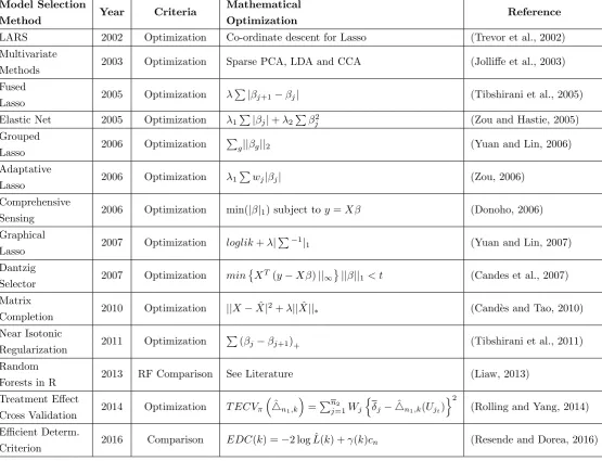
Figure 1: Diabetes Dataset.

This image shows a set of data. The objective of the linear regression is obtaining a linear functionh(x) that best approximates the data. For example:

Figure 2: Diabetes Dataset linear regression.

In this graph the blue line represents the function h(x) that was mentioned before.

This case, as it can be seen, is rather simple. The regression only estimates two variables, a constant ( 0) and a coefficient ( 1). However, as it will be seen later,

log-likelihood function. This is explained in the following subsection.

Log-Likelihood

The maximum likelihood estimate is a statistical measure that is the result of the max-imization of the likelihood function. This maxmax-imization does not necessarily assume that the parameters are under a prior distribution, but instead, they assume that their estimates do. Given a prediction for the sample iwe have that:

h xi0, xi1, ..., xip = 0xi0+ 1xi1+...+ pxip+✏i (3)

In this equation X and Y do not necessarily have a specific distribution. Being✏i_{the residual of each data point (x}i

0, xi1, ..., xip, yi) independent from each other

and following N (0, 2_{), and assuming the linearity of the function h (x). Then}

the likelihood function (having p, number of explanatory variables andn number of samples) given the dataset xi

0, xi1, ..., xip where iis the observation from 0 to nbegin

nthe last observation:

L( |x) =p (x) =

n

Y

i=1

p(yi|xi; 0, 1, ..., p, 2) (4)

Assuming that the distribution of the residuals✏i_:

L( |x) =

n

Y

i=1

1 p

2⇡ 2e

(yi h (xi))2

2 2 (5)

Using basic logarithm properties this equation can be written as:

logL( _|x) =

n

X

i=1

logp(yi_|xi; 0, 1, ..., p) (7)

And then its maximization:

argmax

n

X

i=1

logp(yi_|xi; 0, 1, ..., p)

!

(8)

When the prior probability distribution of the estimates is taken under the assumptions mentioned before is assumed , then solving the previous equation:

argmax

n

X

i=1

log_p 1 2⇡ 2e

(yi h (_xi))2 2 2

!

= (9)

argmax n

2 log 2⇡ nlog 1 2 2

n

X

i=1

(yi h (xi))2

!

(10)

Which leads to the minimization (over ) of:

n

X

i=1

yi h (xi) 2 (11)

The result of this equation is a set of parameters (or coefficients) ( 0, 1, ..., p)

that define the regression functionh (x). Equation 11 shows themean square error of the fitted data is what is trying to be optimized. This function is also commonly called cost function. Optimizing this function lead to the values of that lead to a lower mean square error

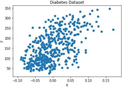
Cost function and gradient/coordinate descent algorithms

The cost function is a function which value can be interpreted as a measure of fit of the model. It measures the mean square di↵erence between the estimations and the real values of the data. This function is generally written as:

J( 0, 1, ..., p) =

1 2m m X i=1 ⇣

h (x(i)) y(i)⌘2 (12)

It is directly intuitive that the lower the cost function the better the line fits the data. Therefore, the objective of the linear regression will be:

argmax 0, 1,..., p

1 2m m X i=1 ⇣

h (x(i)) y(i)⌘2

!

(13)

As an example,diabetes data set will be used. In the case only two variables were considered, a constant ( 0) and a coefficient ( 1). The cost function in this case

will be:

J( 0, 1) =

1 2m

m

X

i=1

(h (xi) yi)2

!

(14)

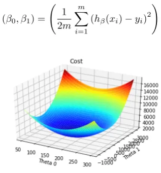
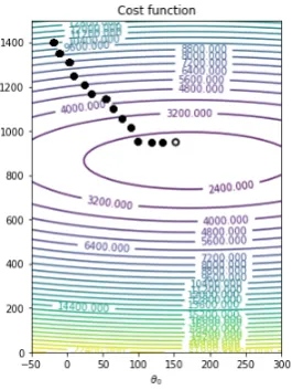
function. The most common is calledgradient descent. This algorithm is very intu-itive, it performs a sequence of iterations that updates for values in which the cost function is lower. Roughly speaking it is as if we drop a ball in a point of the function and watch where the ball ends up. The iterative process for thediabetesdataset would be:

0:= 0

@ @ 0

J( 0, 1) (15)

1:= 1 @

@ 1

J( 0, 1) (16)

In this equation it can be seen that the parameters 0 and 1 are being

learned to find the minimum value of the cost function. In the equation the value is the distance of each step taken in the update. The value of must be chosen carefully. Large values of could lead to miss the cost function minimum. Normally, built-in functions use a small value of . The learning process can be visualized in the 3D:

In a contour plot:

Figure 5: Contour plot.

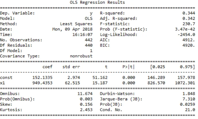
Figure 6: Results from Linear Regression on Diabetes Dataset.

The results just shown give the coefficients necessary to get the prediction functionh (x) (seeFigure 2, the blue line):

h (x) = 0+ 1x1= 152.1335 + 949.4353x (17)

4.3

Logistic Regression

Logistic regression is a mathematical modelling process in which a relationship is established between an output Y (which is a logical dependent variable, Boolean 0 or 1) and a set of explanatory variables. The variableyi _{is called dependent or response}

variable Seber and Lee (2012) and (x0, x1, ..., xp) explanatory or independent variables

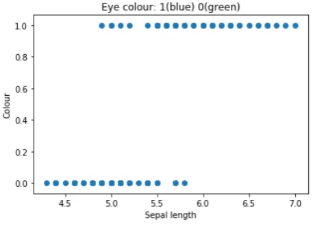
Seber and Lee (2012). The main di↵erence between linear and logistic regression is that the output variable is discrete. I takes values: 0, 1, 2 ,... etc. In this section we will consider onlybinary classification problem, in which the output is either1 or

0. The reason for this is that the models we are going to study in this thesis are PD Models which outputs are 0: Non-Default or 1: Default. Also it can serve for Cure Models with0: Not cured or1: Cured. In the following example we consider a dataset that contains data from di↵erent eyes, which final output is the eye colour (green or blue):

The previous image shows how data is classified in two sets (0 and 1). Intu-itively attempting classification using linear regression is a bad idea because the output does not take values higher than one (in binary classification problems). Therefore the

linear regression function:

h(x0, x1, ..., xp) = 0x0+ 1x1+...+ pxp, (18)

is plugged into the Sigmoid function (g(h (X))):

g(h (X)) = 1

1 +e h (X). (19)

Figure 8: Sigmoid Function.

This function gives the probability that the output is 1. So basically, logistic regression is a linear classifier. Therefore if we consider the transition from linear to logistic this would be:

h (x)linear)g(h (x)linear) (20)

regression. This is due to the prior distribution we assume that the output has. Nevertheless, the parameters are estimated maximizing the likelihood function, as in linear regression.

Log-likelihood

First of all, we must notice that logistic regression predicts probabilities. The likelihood then is

L( 0, 1, ..., p) =

n

Y

i=1

p(yi|xi; 0, 1, ..., p), (21)

and taking into account the distribution of this probabilities (Bernoulli) we have that

L( 0, 1, ..., p) =

n

Y

i=1

p(xi)yi(1 p(xi))1 yi, (22)

and taking logarithms to make the maximization easier we have that

log(L( 0, 1, ..., p)) = n

X

i=1

yi_logp(xi_{) + (1 y}i_{) log((1 p(x}i_{))). (23)}

The maximization of the log-likelihood (which is the same as maximization of likeli-hood) is done in order to obtain the parameters that best fit the data. Having that:

p(x(i)) = e

0+ 1x(i)1 +... px(i)p

1 +e 0+ 1x(i)1 +... px(i)p

= 1

1 +e ( 0+ 1x(i)1 +... px(i)p )

=g(h (x)) (24)

The minimization of this function is done the same way as in linear regression, us-ing coordinate descent or gradient descent. The result of this minimization are the parameters of the vector ( 0, 1, ..., p) that define the regression logistic model.

4.4

Conclusion

In this section we have made an introduction to the two main types of regression methods: linear and logistic. Each of them serves to a di↵erent estimation purpose and therefore fitted in a di↵erent way. The implementation of these regression types has been summarized for the reader to get familiarized with the implementation methods such as gradient descent and coordinate descent. Also it is important to get the idea of the derivation of the log-likelihood function to obtain the cost function for each of the estimation types. This is so, because the model selection algorithms developed in

5

Model selection

5.1

Introduction

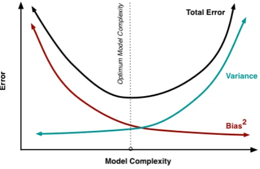
In the last section, two main types of regression were presented as well as some concepts used for their estimation. This has to be the first step when modelling: identifying the nature of your data. Secondly, a modeler must think carefully about the purpose of the model: explanatory (fit) or prediction. Paradoxically, a model that has a very good fit on the existing data may not be the best model for prediction. This is issue has been addressed several times in statistical modelling. One of the reasons for this to happen is overfitting.

Overfitting occurs when the regression models sticks too much to the data used for the model. It is illustrated in the following picture:

Figure 9: Overfitting (source: Wikipedia).

The image shows a binary classification regression fitted by two di↵erent models. Green model fits the data closely and this results in a high explanatory power. However it leads to a higher error on prediction with new data samples. This means that the green model has a low bias (close to reality) but a high variance (poor predictive power). On the contrary the black model is not that close to the existing data (meaning high bias) but has a better predicting power (low variance).

Intuitively we can think of variance and bias as error measures of our model. In the previous section we introduced the Cost Function expressed as the error as-sociated with our model regarding the observations and predictions. This error was calculated in a di↵erent way for logistic and linear regression. In fact, this error can be decomposed into variance and bias. The mathematical demonstration can be found in Sammut and Webb (2017) and it will not be shown here. The result of the decom-position of thetotal error is:

E[Error] =V ar[noise] +bias2+V ar[yi] = 2+bias2+V ar[yi] (26)

There is a direct relationship between model’s complexity and total error (as a sum of variance and bias). This relationship mentioned previously in this section can be plotted as follows:

Figure 10: Variance Bias Trade-o↵(Fortmann-Roe, 2012).

The need for model selection

5.2

Model Selection by comparison

If we recallFigure 6, few parameters were estimated for the diabetes dataset with their correspondent value. Some of these parameters are actually a score of the model. Their values can be used for performing model selection based on comparison to models that fit the same data. In this thesis, the parameters that will be used for comparison will be:

• R squared

• AIC

• BIC

• P values

5.2.1 Akaike Information Criterion

When model’s quality is assessed only by referring to fit, usually the model with more explanatory variables will always be chosen. However, this is not necessarily good. When a model uses too many parameters, overfitting5_{may occur. AIC raises to solve}

the problem of overfitting. It is an statistical measure developed by Akaike (1974) that asses model quality by calculating the AIC factor. It takes into account the log-likelihood estimation and the number of variables to be consider for regression. This factor can be expressed as:

AIC= 2k 2ln( ˆL), (27)

being ˆL the value of the maximum of the likelihood function and k the number of parameters in the model.

The Akaike Information criterion is the derivation of Mallow’s CP if the

residuals are normally distributed. This score is an estimate of the fit of the model (as it is derived from the log-likelihood), but taking into account the number of variables included. It is a relative measure so it is useful only when models are compared. The

model with the lowest AIC value is considered to be better. Therefore this measure is only useful for situations in which di↵erent models need to be compared.

However, AIC raises a problem when the number of observations is low, because then the correction of 2k is not enough for penalizing large models, this was shown in the paper (Hurvich and Tsai, 1989). Therefore a correction was developed by (Cavanaugh, 1997) for situations with small number of samples. The formula for the corrected version of the Akaike Information criterion is:

AICc =AIC+ 2k

2_{+ 2k}

n k 1. (28)

This formula must be used for when the sample is small. However when the sample tends to be big the extra penalty tends to 0, turning AICc into AIC. The

following graph shows the comparison between both measures when applied to the diabetes dataset with few samples:

Figure 11: Comparison betweenAIC andAICc.

5.2.2 Bayesian Information Criterion

BIC also addresses the problem of overfitting by penalizing the log-likelihood estimate for models with higher complexity. The di↵erence between BIC and AIC is that BIC takes into account the number of samples used in the model, even when the number of samples is big or small. the equation for calculating the BIC can be written as:

BIC=ln(n)k 2ln( ˆL), (29)

being ˆLthe value of the maximum of the likelihood function,n the number of samples and k the number of parameters in the model. As we can see in the equation AIC is similar to BIC. The only di↵erence is that AIC uses a penalty of 2k while BIC uses ln(n)k. This can be shown in the following graph:

Figure 12: Comparison betweenAIC andBIC.

5.2.3 R-squared

R-squared or the coefficient of determination can be intuitively defined as how good the variance of the model explains the variance of the data. It is also usually a measure of the goodness of fit of the model, representing how well does the model fit the data.

Linear Regression

R2_{= 1} V ARmodel

V ARdata

(30)

Its value is between 0 and 1, however, in occasions in which a very bad fitting model is chosen, this coefficient can even be out from this interval. R-squared increases every time a variable is included in the model, this is logical since the more explanatory variables in the model the best the data is fitted. However, this is is not necessarily good, since sometimes variables that are included in the model, even if they increase the simple R-square, they are rather not significant enough for the model.

Logistic Regression

In logistic regression, R-squared (called McFadden’s pseudo R2) is defined as:

R2= 1 L( ˆ) L(0)

!2/n

, (31)

where L(0) is the log-likelihood of the null model, L( ˆ) is the log-likelihood of the optimized model and n the number of samples. This definition of R-squared makes sense for the boundries ofR2_{. When the estimated model is as bad as the null model,}

R-squared is 0 and when the log-likelihood of the estimated model is 0 (this is thetrue model), R-squared is 1.

To fix this problem extensions of R-squared are considered for model comparison with di↵erent number of explanatory variables, there is a way to adjust R-squared. This is the so called R-squared adjusted. It is defined as:

R2adj = 1 (1 R2)

n 1

n p 1 (32)

In whichnis the number of samples,Ris the regular R-squared andpis the total number of explanatory variables. In the following graph the comparison between the non-adjusted and the adjusted can be seen:

Figure 13: Comparison between R-squared and R-squared adjusted.

In the previous graph it can be seen how the adjusted R-squared decreases slightly. This adjustedR2_{can perform model selection by comparing two models that}

fit the same data but with di↵erent model complexity.

5.2.4 Stepwise Regression

Background

Stepwise Regression was developed by Efroymson (1960). It is a combination of For-ward and BackFor-ward Regression. These algorithms work as follows:

• Forward Regression: the initial model contains no variables. Then all variables are considered for inclusion and the one that has the lowest p value is included in the model only if this p-value is lower than a given thresholdp-enter. Afterwards, all the resting variables are considered again and the one that in combination with the first variable has a the lower p-value (and also lower than the threshold) is included in the model. The algorithm goes on and on till no variable makes the model significantly better.

• Backward Regression: the initial model contains all variables. Then variables are sequentially eliminated if their p-value is higher than a given thresholdp-remove. When a variable is removed, the model is fitted again and all variables checked. The algorithm stops when no variable in the model has a higher p-value than

p-remove.

Algorithm

Stepwise regression is a model selection method based on comparison. Each step of the algorithm considers each variable for inclusion to the model (forward) and all variables in the model for exclusion (backward). The addition of variables to the model is executed when a variable has pvalue lower than the p value threshold, to be specified by the user (by default 0.05). The exclusion of variables from the model is executed when a variable has a pvalue higher than the p value threshold, to be also specified by the user (by default 0.10).

selection starts with all variables in the model and eliminates one by one variables that are not significant for the model, given a threshold.

Stepwise regression is a combination of this two model selection methods. It sequentially performs forward and backward till no change significantly improves the model. Long story short, forward considers variables for inclusion and backward

5.3

Model Selection by optimization

The previous model selection algorithms where based on comparison of models fitted by maximizing the Log-likelihood (minimizing cost function), and once the parameters and the maximum Log-likelihood are obtained the scores were calculated. These scores were use then to determine which model is the best (in case ofAIC, BICand R2

adj)

or also to serve as an input for a more complex model selection algorithm (such as the p-values with stepwise regression).

However, some model selection methods perform variable selection from the moment the parameters are estimated. This is that they minimize a di↵erent ’cost function’ in order to perform model selection. As shown in the literature review ( Sec-tion 2) there are several methods for model selection by optimization. Nevertheless, in this section we will only focus in least absolute shrinkage and selection operator

(Lasso) and Elastic Net due to the reasons explained inSection 2.

5.3.1 Lasso

We can recall from Section 4.2 that finding the minimum of

argmin 0, 1,..., p m

X

i=1

⇣

h (x(i)_{) y}(i)⌘2

!

(33)

leads to obtaining the coefficients for the parameters in linear regression that best fit the data. However, as it was said at the beginning of this section finding the best fit is not a good idea if the purpose of our model is prediction.

The Lasso, performs shrinkage and variable selection by solving thel1-penalized

regression problem (Tibshirani, 2011) on finding

argmin 0, 1,..., p

0 @ m X i=1 ⇣

h (x(i)_{) y}(i)⌘2₊

p

X

j=1

| j|

1

(parameters can shrink to 0) depending on the value of the l1-penalty, . The

fol-lowing graph shows how this penalty shrinks the parameters and performs variable selection when estimating a model for the diabetes dataset, that contains 10 variables:

Figure 14: Performing variable selection for the diabetes dataset using Lasso

In the previous figure it can be seen how for higher values of model com-plexity becomes smaller. The only value necessary to adjust for implementing Lasso is . Traditionally, this penalization parameter must be chosen manually by the user, but this be done carefully. As it was shown in Figure 14 the shrinkage of the param-eters is not the same for all, some of them shrink faster and some slower, leading to di↵erent results (errors, variance...) in the final model. Later on, inSection 7 we will propose an automatic method to chose the value of the penalization.

5.3.2 Elastic Net

Elastic Net is a generalization ofleast absolute shrinkage and selection operator (Lasso) that combines an l1 penalty with al2 penalty (Ridge Regression). It was a method

proposed by Zou and Hastie (2005) to solve three limitations that Lasso had (Zou and Hastie, 2005):

Lasso selects at most n variables variables

• Correlation: if there is a group of variables highly correlated, Lasso tends to select one variable from the group and disregard the rest

• Case n p. In cases where the number of observations is higher than the number of variables (which is usually the case) and there are high correlations among the variables, Ridge Regression has a better predictive power.

Elastic Net performs as well variable selection and parameter shrinkage by performing the minimization of the function:

argmin 0, 1,..., p

0 @ m X i=1 ⇣

h (x(i)) y(i)⌘2+ ↵ p

X

j=1

| j|+ (1 ↵) p

X

j=1

| j|2

1 A (35)

which is basically minimizing the cost function plus two additional terms (l1

-penalty (Lasso) and l2-penalty (Ridge)). The value of↵ is to be chosen by the user

and represents the proportion from each penalty to be used in the optimization. If ↵

Figure 15: Performing variable selection for the diabetes dataset using elastic net with

↵= 0.9.

5.4

Conclusion

We presented a model selection framework that divides model selection algorithms into two types: model selection by comparison (Section 5.2) and model selection by optimization (Section 5.3). Afterwards, several model selection algorithms have been explained with examples in order to see how do the di↵erent procedures perform variable selection.

Model Selection

Criteria Comments

Comparison

BIC Select model with

highestBIC

AIC Select model with

lowestAIC

R2

adj

Select model with highestR2

adj

Stepwise Selects model that does not significantly improve the fit

Optimization Lasso

min⇣Pm_i=1 h (x(i)_{) y}(i) 2₊ Pp j=1| j|

⌘

subject to Pp_j=1| j|s

Elastic Net min

⇣Pm

i=1 h (x(i)) y(i) 2+ (1 ↵)

Pp

j=1| j|+ ↵Ppj=1| j|2

⌘

subject to (1 ↵)Ppj=1| j|+ ↵Ppj=1| j|2s

Table 3: Model Selection framework.

6

Model Validation

6.1

Introduction

In previous sections we discussed model estimation (logistic and linear regression) and some model selection procedures (AIC,BIC, Stepwise, Lasso...). Model estimation methods are necessary to understand in order to be able to identify data type and to understand estimation procedure. Also and equally important is to choose the model that aims to describe how data are generated (model selection). When the goal of these models is prediction, it is desired that the model’s accuracy with new data is high. However sometimes the data used for training the model does not significantly represent all sets of data (it can be biased). Therefore, models that have been trained with some data must be validated. Cross validation is a well-known common technique for model validation which basically consists of partitioning a set of data into a training set and a validation set. The training set is used to fit the data and estimating the value of the parameters and the validation set is used for calibration (or evaluation) of the model. If the performance of the model in the validation set is good enough, there is no need for model calibration. However, if there is some error in the validation set, the modeler has to calibrate the parameters of the trained model taking into account the results from the validation set. For example, the validation set can be used for calibrate the regularization coefficient or the↵ratio for Elastic Net.

There are several methods for partitioning data for cross validation models. The conventional way is partitioning data in two sets: 70% training and 30% validation. However if the partitioning is done randomly it can occur that the training set di↵ers a lot from the validating set. For example, if we want to model Probability of Default, it would be very inefficient if all non-defaulted loans are in the training set, and all defaulted loans are in the validation set.

6.2

Leave One Out

Leave One Out is a method of cross validation that partitions the data sample by sample. Suppose we have a dataset with a number of samplesn. This method divides the data in n 1 training set and 1 as a validation set. This is done n times for each sample, so each sample will eventually become a validation set. In the following example we will train the diabetes dataset using Lasso Model Selection and we will calibrate the regularization coefficient↵ using Leave One Out Cross Validation. For each value of ↵, n models are trained and validated using the resting sample. The mean error from the validation of each sample is taken:

Figure 16: Leave One Out Cross Validation.

As it can be seen in this case we are calibrating alpha. The calibration is done in the following way:

• For each sample i, a model is trained excluding that samplei, and usingn i as a training set.

• The error in the prediction of that sampleiis computed for each value of↵

because it is computationally very expensive to run n di↵erent models for datasets with very large number of samples. This issue will be addressed in Section 9 when using Leave One Out Cross Validation to calibrate the value of ↵in Lasso Regression

6.3

K-Fold

K fold uses the same underlying idea of Leave One Out, but it does bigger partitions, and thus it becomes less computationally expensive. Namingkas the number of folds (data partitions), the samples are divided into k di↵erent folds. Then, the model is trained k times using n/(k 1) samples as a training set and n/k samples as a validation set. Then the procedure for calibrating the model is the same as in Leave One Out but instead for each sample, for each fold.

Figure 17: K Fold Cross Validation using 3 folds.

The number of folds is an important consideration to take into account. No-tice that when k ₎n K fold turns into Leave One Out. If we increase the number of folds the ↵selected will asymptotically converge to the ↵calculated in Leave One Out:

Figure 18: K Fold Cross Validation using 100 folds.

introduction of these section about the percentage of output type in the folds. The solution to this problem is presented in the next section.

6.4

Stratified K-Fold

Figure 19: Stratified K Fold Cross Validation using 3 folds.

6.5

Conclusion

7

Specifications for chosen model selection algorithms

7.1

Introduction

This section will present the algorithms that haven been programmed in order to test the model selection algorithms that want to be compared. If we recall these algorithms were Stepwise, Lasso, Elastic Net, BIC, AIC and Radj.

The first algorithm will be built to test Stepwise Regression. It combines For-ward selection and BackFor-ward elimination with di↵erent features to be adjusted by the user. The second algorithm called Bruteforce will test all the possible combinations of variables and will select the one that scores the best AIC, BIC,Radjor Log-Likelihood

(criterion must be specified by the user). The third algorithm combines Lasso shrink-age with automatic calibration of the penalization parameter via cross validation (CV method to be chosen by the user). The last algorithm performs Elastic Net with automatic calibration of the penalization and ↵.

7.2

Stepwise Regression with stopping criteria

Stepwise regression is a combination of this two model selection methods. It sequen-tially performs forward and backward till no change significantly improves the model. The algorithm forward considers variables for inclusion and backward considers the selected variables from forward for exclusion. This function has been programmed in Python and also it has been tailored for Rabobank purposes, and thus, includes special features. These are:

• White List: List of variables that are forced to be included in the model.

• Sign: Variables in the final model will only have a concrete sign.

• P-remove: Minimum p-value that specifies the min o p-value for a predictor to be recommended for removal.

• Stopping criteria: Stopping criteria based on optimum BIC or AIC.

• Maximum number of variables: Maximum number of variables allowed to be in the model.

The algorithm can be represented as:

Figure 20: Stepwise algorithm.

7.3

Bruteforce

Bruteforce is an algorithm that given a dataset finds the best combination of features following a specific criterion. This criterion must be selected by the user, there are four options:

• AIC: Akaike information criterion (chooses the model with the lowest AIC score).

• BIC: Bayesian information criterion (chooses the model with the highest BIC score).

• R2

• Log Likelihood(Chooses the model with the highest Log-Likelihood)

Given a set of data, Bruteforce rotates all possible combinations of attributes using the variables given without exceptions.

This function can be computationally very expensive, thus, is recommended not to apply Bruteforce to very large datasets. Instead, other selection methods can be used, such as Lasso Elastic Net or stepwise.

Figure 21: Bruteforce algorithm.

7.4

Post Lasso CV

Post Lasso CV performs Lasso model selection for a given set of data for di↵erent values of the regularization parameter (alpha). The dataset is cross validated to calibrate the value of the regularization parameter in order to get the value of ↵ that gives the lowesterror for the resulting model.

7.4.1 Background

The error in regression methods is usually a decisive factor to choose for one method or another. Typically, the mean square error is an indicator of the model quality. If we recallEquation 26 that explained the demonstration of (Sammut and Webb, 2017):

E[(y f0)] = 2+var[f0] +bias[f0]2 (36)

The variance in itself measures the prediction power of our model. In other words, how accurate is the prediction. On the other hand, bias measures how far is our data from reality. A straight forward reasoning would be concluding that the best model is the one with low variance and low bias. But this is not as easy as it seems. Models that are estimated maximizing the Log-likelihood function, usually fit good the data, achieving a low bias in the model. However, the price of model’s fitted in this way is a poor predictive power. Lasso, Ridge and Elastic Net partially fix this problem by introducing a regularization parameter that reduces overfitting, by penalizing variables that are not very significant for the model. Lasso and Elastic Net also perform variable selection by penalizing some variables to 0 (which Ridge does not), reducing model’s complexity. However, the price to pay for this if the regularization parameter is to high is a high bias in the model.

7.4.2 Purpose

minimum of this function by computing the average error across the cross validation folds for di↵erent values of the regularization parameter.

Figure 22: Variance - Bias Trade o↵.

As it can be seen we will start with a Lasso model with = 0 (which is the same as saying OLS for linear regression) and increase alpha sequentially till we have the whole picture, for finally select the optimum model.

7.4.3 Algorithm

Figure 23: Variance - Bias Trade-o↵.

7.4.4 Example

Using the diabetes dataset we perform PostLassoCV using Stratified K-fold cross val-idation method with 5 folds. The result from the function is:

If we look carefully at the graph we can even identify the variance bias trade-o↵in the average mean squared error across the folds:

Figure 25: Final Post Lasso CV.

As we can see Post Lasso CV will select the value of↵that gives the lowest Total Error leading to a higher prediction power of the model. As explained previously in last section this graph shows the error across the folds (in this case 5 folds), and the average of these errors (the thick black line). This cross validation method aims to simulate the variance-bias trade-o↵to be able to choose the lower error point. If alpha is set to 0, we will have a traditional model with all variables, if we increase the value of alpha we will be shrinking variables to 0 (See Figure 14), and thus, progressively as alpha becomes very big, there will be no model (or constant 0 model), which leads to high error.

7.5

Elastic Net CV

This function is a generalization of the previous Post Lasso CV that adds another dimension to the optimization of the model selection algorithm. It will rotate the penalization parameter as well as the regularization and select the situation in which the error is lowest for the model.

7.6

Conclusion

In this section we have presented four algorithms that perform model selection (& calibration in Post Lasso CV and Elastic Net Cross Validation case). These algorithms di↵er slightly from the conventional ones. In the case of Stepwise Regression, the algorithm includes more input features that can be manipulated to obtain a better result. Bruteforce gives the chance to vary the selection criteria in order to evaluate the model selection.

Post Lasso CV and Elastic Net Cross Validation perform automatic calibra-tion for convencalibra-tional Lasso and Elastic Net procedures and output the final calibrated model and the regularization (and penalization for EN) parameter.

8

Testing

8.1

Introduction

In this section we are going to test data from Rabobank. Because of confidential rea-sons neither thenature of this datanor thename of variableswill be mentioned. Instead, all variables will be named as (x0, x1, ..., xp) beingpthe variable index.

Firstly, the type of data is going to be slightly introduced, however not in much depth as it was mentioned before. Then the testing method framework is going to be described for the reader to understand the methodology followed for comparing each selection procedure. The chapter will end with a conclusion that ties up the testing procedure and its reasoning. Next section will present the results of this testing.

8.2

Data

The data that are going to be use for testing have the format of a matrix of nxp:

0 B B B B @

x0,0 x0,1 . . . x0,p

x1,0 x1,1 . . . x1,p

..

. ... . .. ... xn,0 xn,1 . . . xn,p

1 C C C C A

where in our casen(= 43381) is the total number of samples andp(= 26) is the number of variables to be considered. Also, we will have the column of outputs (dependent variable)y: 0 B B B B @ y0 y1 .. . yn 1 C C C C A

8.3

Testing procedure

The testing criteria have been developed taking into account the model selection meth-ods to be considered. These are the ones explained in the previous section: Post Lasso CV,Stepwise Regression andElastic Net CV.

Figure 26: Testing procedure.

Figure 27: Data Usage.

Additionally, these functions have also some optional input parameters that may a↵ect the implementation of the algorithm and thus, the outcome model. There-fore these input parameters will be also be evaluated when executing the model selec-tion funcselec-tions.

8.4

Conclusion

9

Results

9.1

Introduction

In the following section the testing results are going to be presented. For each model selection procedure there are di↵erent input parameters that can be adjusted. Natu-rally the outcome depends on these parameters, and thus this will be tested as well.

For stepwise regression the p-value thresholds will be modified in order to find the combination ofp-enter andp-removethat gives the best model. Also for Post Lasso CV the coefficient threshold for variable selection will be as well modified. The performance of both algorithms will be compared also in a test set as explained in the last section.

Finally we are going to make a fairer comparison between both using Stepwise and PLCV as model selector algorithms and calculating the accuracy ratio predicting in di↵erent folds and also the selection progress. This will give a robust ratification of the comparison.

9.2

Stepwise regression model

p enter

p remove 0.05 0.1 0.15 0.20 0.25 0.3 0.35 0.45 0.010 49130.5 49130.5 49130.5 49130.5 49130.5 49130.5 49130.5 49130.5 0.025 49130.5 49130.5 49130.5 49130.5 49130.5 49130.5 49130.5 49130.5 0.050 49130.5 49130.5 49130.5 49130.5 49130.5 49130.5 49130.5 0.075 49129 49129 49129 49129 49129 49129 49129 0.100 49129 49129 49129 49129 49129 49129 0.125 49129 49129 49129 49129 49129 49129 0.150 49128.9 49128.9 49128.9 49128.9 49128.9 0.175 49128.9 49128.9 49128.9 49128.9 49128.9 0.200 49128.9 49128.9 49128.9 49128.9 0.225 49128.9 49128.9 49128.9 49128.9 0.250 49128.9 49128.9 49128.9

0.300 49128.9 49128.9

0.350 49128.9

0.450

p enter

p remove 0.05 0.1 0.15 0.20 0.25 0.3 0.35 0.45 0.010 16 16 16 16 16 16 16 16 0.025 16 16 16 16 16 16 16 16 0.050 16 16 16 16 16 16 16 0.075 17 17 17 17 17 17 17 0.100 17 17 17 17 17 17 0.125 17 17 17 17 17 17 0.150 18 18 18 18 18 0.175 18 18 18 18 18

0.200 18 18 18 18

0.225 18 18 18 18

0.250 18 18 18

0.300 18 18

0.350 18

0.450

Table 5: Degrees of Freedom.

p enter

p remove 0.05 0.1 0.15 0.20 0.25 0.3 0.35 0.45 0.010 -24548.2 -24548.2 -24548.2 -24548.2 -24548.2 -24548.2 -24548.2 -24548.2 0.025 -24548.2 -24548.2 -24548.2 -24548.2 -24548.2 -24548.2 -24548.2 -24548.2 0.050 -24548.2 -24548.2 -24548.2 -24548.2 -24548.2 -24548.2 -24548.2 0.075 -24546.5 -24546.5 -24546.5 -24546.5 -24546.5 -24546.5 -24546.5 0.100 -24546.5 -24546.5 -24546.5 -24546.5 -24546.5 -24546.5 0.125 -24546.5 -24546.5 -24546.5 -24546.5 -24546.5 -24546.5 0.150 -24545.4 -24545.4 -24545.4 -24545.4 -24545.4 0.175 -24545.4 -24545.4 -24545.4 -24545.4 -24545.4 0.200 -24545.4 -24545.4 -24545.4 -24545.4 0.225 -24545.4 -24545.4 -24545.4 -24545.4 0.250 -24545.4 -24545.4 -24545.4

0.300 -24545.4 -24545.4

0.350 -24545.4

0.450

p enter

p remove 0 0.05 0.1 0.15 0.20 0.25 0.3 0.35 0.010 0.494885 0.494885 0.494885 0.494885 0.494885 0.494885 0.494885 0.494885 0.025 0.494885 0.494885 0.494885 0.494885 0.494885 0.494885 0.494885 0.494885 0.050 0.494885 0.494885 0.494885 0.494885 0.494885 0.494885 0.494885 0.075 0.495013 0.495013 0.495013 0.495013 0.495013 0.495013 0.495013 0.100 0.495013 0.495013 0.495013 0.495013 0.495013 0.495013 0.125 0.495013 0.495013 0.495013 0.495013 0.495013 0.495013

0.150 0.49514 0.49514 0.49514 0.49514 0.49514

0.175 0.49514 0.49514 0.49514 0.49514 0.49514

0.200 0.49514 0.49514 0.49514 0.49514

0.225 0.49514 0.49514 0.49514 0.49514

0.250 0.49514 0.49514 0.49514

0.300 0.49514 0.49514

0.350 0.49514

0.450

Table 7: Accuracy Ratio (Training Set).