NIR spectroscopy for personal screening

(1)

A Thesis Submitted for the Degree of PhD at the University of Warwick

http://go.warwick.ac.uk/wrap/49178

This thesis is made available online and is protected by original copyright. Please scroll down to view the document itself.

(2)

b

y

A

a

m

e

r

S

a

l

e

m

S

SuubbmmiitttteeddffoorrtthheeddeeggrreeeeooffPPhh..DD..iinnEEnnggiinneeeerriinnggttootthheeUUnniivveerrssiittyyooffWWaarrwwiicckk d

deessccrriibbiinnggrreesseeaarrcchhccoonndduucctteeddiinntthheeSScchhoooollooffEEnnggiinneeeerriinngg

(3)

List of figures

Chapter 1

1.1 The electromagnetic spectrum, illustrated on a logarithmic wavelength scale.

1.2 The infrared region, subdivided into near, mid and far-infrared.

1.3 A simple diatomic oscillator.

1.4 Potential energy curve for the harmonic motion of a diatomic oscillator.

1.5 Vibrational energy levels of a harmonic diatomic oscillator.

1.6 Vibrational energy levels and permissible transitions of (a) a harmonic diatomic

oscillator, and (b) an anharmonic oscillator.

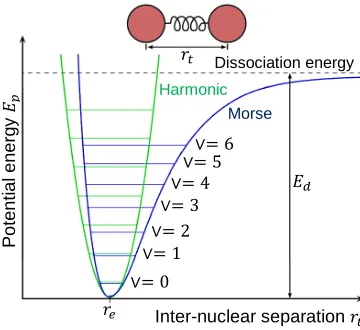
1.7 Potential energy curve for a harmonic oscillator, and the Morse curve for an

anharmonic diatomic oscillator.

1.8 The layout of spectral absorption bands in the NIR region, comprising higher

order overtones and combinations of fundamental transitions.

1.9 Stretching and bending vibrational modes in a CO2molecule.

1.10 Different methods of presenting samples, including transmittance, reflectance,

transflectance and interactance, used to collect NIR spectral data.

Chapter 2

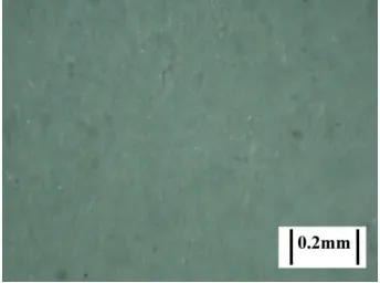
2.1 Sheet of 80gsm paper imaged under a light microscope.

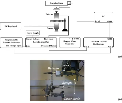
2.2 Arrangement used to detect beam cross-section in x-y plane parallel to the paper

samples and perpendicular to NIR beam axis (z-axis). (a) Schematic diagram of

the apparatus, and (b) photograph of the sample and optical source (laser diode)/

detector.

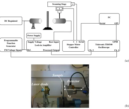
2.3 Arrangement used to detect beam cross-section in x-z plane parallel to NIR

beam axis and normal to the paper samples. (a) Schematic diagram of the

apparatus, and (b) photograph of the sample and optical source (laser diode)/

detector.

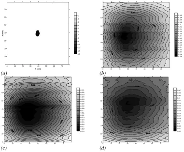
2.4 Cross-sectional intensity scans recorded in the x-y plane across (a) free space,

and (b)-(d) 1-3 layers of paper respectively.

2.5 Results of cross-sectional line scans across 1-40 sheets of paper; (a) Normalized

intensity curves; (b) FWHM values for the curves in (a).

(8)

beam, recorded across (a)-(c): 1-3 layers of paper respectively.

2.7 Signal decay across paper samples along the direction of travel of the beam

(z-axis), recorded using the arrangement in Figure 2.3. (a) Characteristic plots for 2

sheets of paper; (b) α_୔_{_}_୅୴୥for 1-5 layers of paper.

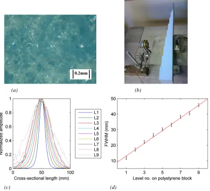
2.8 Measurements with polystyrene sample; (a) Sample imaged with light

microscope; (b) Equipment layout; (c) Normalized line scan data (Thickness of

level n = 5n mm); (d) FWHM values measured for the line scan curves shown in

(c).

2.9 SEM images of copper grids used to study the interaction of pores with NIR

energy.

2.10 Scanning arrangement used to make NIR intensity measurements in 3D across

copper grids.

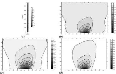
2.11 Cross-sectional contour plots of NIR intensity distribution transmitted through

copper grids with regular pore sizes of (a) 50 μm and (b) 6 μm.

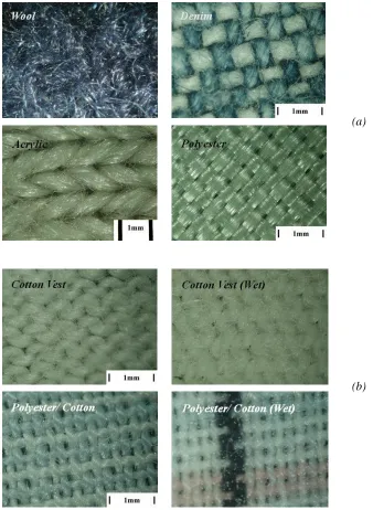
2.12 Optical microscope photographs of (a) four of the fabric samples investigated,

and (b) some fabrics both in the dry state and when moistened with water.

2.13 Studying the characteristics of through-transmitted NIR beam using webcam.

2.14 Intensity-corrected webcam images of NIR beam transmitted through single

fabric layers.

2.15 Point measurements showing drop in NIR intensity across multiple fabric layers.

(W) signifies wet samples.

2.16 Signal variation across various dyed fabric samples of cotton (six colours) and

polyester (black and white only). (W) signifies wet samples.

2.17 Effect of moisture on through-transmitted signal levels.

2.18 Measurements with woollen scarf. (a) Sample imaged with light microscope;

(b) Equipment arrangement; (c) Normalized line scan data for 1-6 layers;

(d) FWHM values measured for the line scan curves shown in (c) (1st value

excluded from linear fit).

2.19 Mass flow meter setup for porosity estimation.

2.20 Variation in porosity with different fabric samples.

2.21 Experiments to measure total transmitted intensity with integrating sphere.

(9)

Chapter 3

3.1 (a) Schematic layout of the optical bench. (b) Photograph of the same arrangement (lens L3 and optical fibre cable were moved back 3 m from the sample before making stand-off spectral measurements).

3.2 Optical bench arrangement depicting the use of a PTFE standard reflection block with liquid samples.

3.3 Photographs of the 14 fabric samples, identified by numbers that correspond to the data in Table 3.2.

3.4 Absorbance spectra of white polyester fabric sample, recorded with two different references. (a) 2nd degree polynomial functions that fit the spectra in a least squares sense. (b) Spectra in (a) after de-trending, illustrating same spectral features in the two cases.

3.5 Spectral response curve of spectrometer (marked NIR256-2.1).

3.6 Spectral saturation due to the first overtone of water (1 450 nm). (a) Spectra of water and two ethanol solutions, showing saturation in the 1 400 – 1 800 nm wavelength range (measured in diffuse reflection with optical path ~20 mm; reference: empty cell with PTFE). (b) Spectra of water for different optical paths (measured in transmission in glass cells of different widths); the first overtone is defined for path lengths up to 1 mm.

3.7 Spectra of water and ethanol solutions in various concentrations, after filtering, translation and range selection (measured in diffuse-reflectance across optical path of 20 mm, with reference to empty cell and PTFE).

3.8 Transmission coefficients of fabric samples listed in Table 3.2. Measurements were made in through-transmission, using an integrating sphere to determine the total integrated transmission intensity over the 900 – 1,300 nm wavelength range.

3.9 Optical microscope photographs of selected fabric samples; (a) white cotton (cotton no. 1), (b) black cotton (cotton no. 3), (c) denim and (d) white polyester. The thickness t of each sample is also shown.

3.10 Absorbance spectra of cotton no. 2 samples (ref. Table 3.2 and Figure 3.8) in both visible (main window) and NIR (inset) wavelength range. Diffuse reflectance measurements were made with reference to 10 mm thick PTFE block. Data were filtered and 1st-degree de-trended.

(10)

spectra for visual clarity.

3.12 Absorption spectra of table sugar (sucrose) and white cotton. Data were collected in diffuse reflectance, filtered and de-trended.

3.13 NIR absorbance spectra of ammonium salts containing nitrate, sulphate and chloride ions (reference: 10 mm thick PTFE block). The measurements were made in diffuse reflectance, filtered and 1stdegree de-trended.

3.14 NIR absorbance spectra of ammonium nitrate and ammonium chloride behind a synthetic check shirt (reference: fabric sample). The measurements were made in diffuse reflectance, filtered and 1stdegree de-trended.

3.15 Absorbance spectra of coarse-grained ammonium nitrate granules (provided by Sigma-Aldrich Ltd) (a) behind synthetic fabrics, and (b) behind natural fabrics. The measurements were made in diffuse reflectance, with reference to the fabric samples. Spectra were filtered, de-trended and normalized.

3.16 Spectral amplitudes of coarse-grained ammonium nitrate (provided by Sigma-Aldrich Ltd) behind different fabrics for varying air gap between the sample and the clothing material. The peak-to-peak amplitude is plotted between the 1 169 nm minimum and the 1 279 nm maximum. This was obtained from filtered and de-trended spectra measured in diffuse-reflectance with reference to the fabric samples.

3.17 Absorbance spectra of water and ethanol in various concentrations, measured with reference to a block of PTFE placed behind (a) an empty cell; (b) a cell containing water.

3.18 Absorbance spectra of water and hydrogen peroxide in various concentrations, measured with reference to a block of PTFE placed behind (a) an empty cell; (b) a cell containing water.

3.19 Absorbance spectra of water and solutions of ammonium nitrate in various concentrations, measured with reference to a block of PTFE placed behind (a) an empty cell; (b) a cell containing water.

3.20 Absorbance spectra of water and ethanol in various concentrations, placed behind different fabric layers, measured in diffuse reflectance with reference to a block of PTFE placed behind (a) an empty cell covered with the fabric sample; (b) a cell containing water, covered with the fabric sample.

(11)

behind different fabric layers, measured in diffuse reflectance with reference to a block of PTFE placed behind (a) an empty cell covered with the fabric sample; (b) a cell containing water, covered with the fabric sample.

Chapter 4

4.1 Absorbance spectra (with reference to incident source intensity)of the four fabric specimens used to conceal the chemical samples.

4.2 Fabric samples as seen through optical microscope.

4.3 Effects of intervening cotton fabric layer on the spectrum of a liquid. Shown are spectra recorded for (a) water only, (b) water concealed behind a fabric layer (cotton), (c) fabric sample placed on its own, and (d) water concealed behind a fabric layer, with the fabric material taken as reference.

4.4 Scores of the first three principal components of the data, which exhibits clustering.

4.5 First three PC scores showing the distribution of training and test sets.

4.6 Classification of test data by NN trained with Bayesian regularization algorithm.

4.7 Pre-processed spectra of hydrogen peroxide with reference to water, used to calibrate the PLSR model; 80 wavelength channels between 850-1,400nm wavelength range. 4.8 PLSR model validation: MSEE and MSECV as functions of model complexity (number

of PLS factors). Global minimum of MSECV (5 factors) was taken as an initial estimate of optimal model complexity.

4.9 Concentration of hydrogen peroxide predicted by 2-factor PLS calibration model. Test data comprised samples of hydrogen peroxide and outlying chemicals including ethanol and ammonium nitrate. Note that sample numbers (x-axis) reflect sample concentrations in the sequence given in Table 4.4.

4.10 Prediction influence plot using 2-factor PLSR calibration model for hydrogen peroxide. Residual spectral variance vs. leverage for 7 calibration objects and 30 test objects. 4.11 Concentration of hydrogen peroxide predicted by a 4-factor PLS calibration model, in

samples hidden behind a layer of polyester fabric. Test data comprised samples of hydrogen peroxide and outlying chemicals including ethanol and ammonium nitrate. Note that sample numbers (x-axis) reflect sample concentrations in the sequence given in Table 4.5.

(12)

Chapter 5

5.1 Schematic diagram of experimental arrangement used for collection and lock-in amplification of NIR spectral data.

5.2 Block diagram of lock-in amplifier used to process spectral data.

5.3 Front panel GUI of scanning software used for collection and lock-in amplification of spectral data over specified target cross-sections. Marked are the panels used to control and indicate the operation of the lock-in amplifier.

5.4 The lock-in amplifier PLL control/ indication panel in the scanning software.

5.5 The lock-in amplifier demodulator and low-pass filter panel.

5.6 Spectra collected with point-scans across a cell containing distilled water; (a) Water without additive spectral noise; (b) Spectral noise from a PET bottle introduced in (a); (c) Result of lock-in amplification of spectra in (b).

5.7 Neural network-based spectral pattern classification of 2D scans across a cell containing distilled water. Classification results with (a) original spectra (no additive noise), (b) spectra collected in the presence of noise (PET bottle), and (c) noisy spectra with lock-in amplification.

5.8 Spectra collected with point-scans across a cell containing distilled water; (a) Water without additive spectral noise; (b) Software-generated uniform white noise introduced in (a) (SNR = -60 dB); (c) Result of lock-in amplification of spectra in (b).

5.9 Neural network-based spectral pattern classification of 2D scans across a cell containing distilled water. Classification results with (a) original spectra (no additive noise), (b) spectra collected in the presence of uniform white noise (SNR = -60 dB), and (c) noisy spectra with lock-in amplification.

5.10 Spectra collected with point-scans across a cell containing ethanol; (a) Ethanol without additive spectral noise; (b) Software-generated uniform white noise introduced in (a) (SNR = -60 dB); (c) Result of lock-in amplification of spectra in (b).

5.11 Spectra collected with point-scans across a cell containing hydrogen peroxide;

(a) Hydrogen peroxide without additive spectral noise; (b) Software-generated uniform white noise introduced in (a) (SNR = -60 dB); (c) Result of lock-in amplification of spectra in (b).

5.12 Spectra collected with point-scans across a cell containing ammonium nitrate;

(a) Ammonium nitrate without additive spectral noise; (b) Software-generated uniform white noise introduced in (a) (SNR = -60 dB); (c) Result of lock-in amplification of spectra in (b).

(13)

spectra (no additive noise), (b) spectra collected in the presence of uniform white noise (SNR = -60 dB), and (c) noisy spectra with lock-in amplification.

5.14 Neural network-based spectral pattern classification of 2D scans across two cells containing hydrogen peroxide and ammonium nitrate. Classification results with

(a) original spectra (no additive noise), (b) spectra collected in the presence of uniform white noise (SNR = -60 dB), and (c) noisy spectra with lock-in amplification.

5.15 Spectra collected with point-scans across a cell containing hydrogen peroxide hidden behind a layer of polyester; (a) Hydrogen peroxide behind polyester, without additive spectral noise; (b) Software-generated uniform white noise introduced in (a) (SNR = -60 dB); (c) Result of lock-in amplification of spectra in (b).

5.16 Spectra collected with point-scans across a cell containing ammonium nitrate hidden behind a layer of polyester; (a) Ammonium nitrate behind polyester, without additive spectral noise; (b) Software-generated uniform white noise introduced in (a) (SNR = -60 dB); (c) Result of lock-in amplification of spectra in (b).

5.17 Neural network-based spectral pattern classification of 2D scans across a cell containing hydrogen peroxide hidden behind a layer of polyester. Classification results with

5.18 Neural network-based spectral pattern classification of 2D scans across a cell containing ammonium nitrate hidden behind a layer of polyester. Classification results with

5.19 Illustration of the ‘majority poll’ method applied to classification data shown in Figure 5.18(c). (a) Original classification results, predicting both ammonium nitrate and hydrogen peroxide. (b) Outcome of edge detection with Canny’s method. (c) Grayscale version of the original image. (d) Binary image, obtained by setting a threshold at 50% gray level in (c).

(14)

List of tables

Chapter 3

3.1 Specifications of components used in the optical bench.

3.2 Samples of clothing fabrics used for testing.

3.3 Chemicals tested for detection in solid and aqueous solution forms.

Chapter 4

4.1 Sample constituents used to gather calibration and test data.

4.2 Datasets used to train and test NN to classify chemical constituents.

4.3 Determination of optimal model complexity: Global minimum of MSECV i.e.

5-factor model was taken as the first estimate, followed by local minimum of

significance level (randomization t-test) for a more parsimonious solution. The

2-factor model was thus chosen as optimal.

4.4 List of chemical samples used to collect spectral data to calibrate and test 2-factor

PLS calibration model for quantifying chemical concentration.

4.5 Samples of chemicals hidden behind a layer of polyester fabric, used for spectral

analysis to calibrate and test 4-factor PLS calibration model for quantifying

chemical concentration.

Chapter 5

5.1 Specifications of components used in the optical bench.

(15)

Acknowledgments

This work would not have been possible without the unflinching, consistent and

invaluable support of Prof. David A. Hutchins. He was always a source of crucial

guidance and insight, while allowing me all the leeway to work on the subjects that I

felt comfortable with. He was extraordinarily patient and understanding whenever I (all

too often) ran up dead ends, and felt desperate and hopeless. It was only through his

constant encouragement and support that the work was finished on schedule.

Additionally, I would be remiss not to mention the pivotal help of Celine Canal with the

experimental work; her expertise in setting up optical bench arrangements was always a

great source of learning and help, and she was always willing to brainstorm new ideas

and avenues of work. Thanks in no small measure are also due to Lee Davis, for his

ready help with resolving any technical issues whenever they arose. My sincere

gratitude also goes to Robert Southgate and Ritesh Gohel for their help with the work,

as well as to all other members of the group, including Yin Xiaokang, Vipin Seetohul,

Prakash Pallav and Chuan Li (Luby) for their support.

Finally, I would be eternally grateful for the unwavering support of my family,

including my wife Fatima and my parents, which allowed me to keep focus and stay

(16)

Declaration

The work presented in this thesis has been carried out by the author, except where

otherwise stated. It has been performed in the School of Engineering, at the University

of Warwick. No part of this work has previously been submitted to the University of

Warwick, or any other academic institution for consideration for a higher degree. All

publications to date arising from this work are listed in the publications section in the

(17)

Summary

This work presents investigations into the use of the near-infrared (NIR) signals to

interrogate, detect and image specific chemical compounds of interest in a security

screening application, including when such compounds are hidden behind single layers

of clothing fabric.

In an initial set of experiments, the mechanisms governing the interaction of NIR

signals with clothing fabrics and similar materials has been studied, in order to account

for the influence of fabric layers when detecting hidden chemicals. Throughout the rest

of the work, NIR spectroscopy has been used as a means to perform qualitative and

quantitative analysis, in order to detect the presence of chemicals, and quantify the

concentration in aqueous solution of liquids.

It has been shown that, while the compounds can be identified on the basis of the

characteristic features that appear in the relevant NIR spectra, the origin and nature of

these spectra necessitate that such identification be performed with a

chemometrics-based approach. Accordingly, multivariate calibration models chemometrics-based on neural networks

and partial least squares regression (PLSR) have been developed to perform the

requisite analyses. Results of calibration and testing with a range of data are reported.

In order to facilitate operation in practical security screening, the development and

testing of a software-based lock-in amplifier is reported, as a mean to enhance the

signal-to-noise ratio (SNR) of the spectral data. It is shown that the amplifier can

process up to 40 wavelength channels in parallel, to extract the spectral data buried in

noise in each channel. Hence, with the SNR of the input signal set as low as -60 dB (by

introducing software-generated additive white noise in the spectra), adequate noise

suppression has been obtained, allowing the resulting spectral data to be used for

requisite chemical detection.

Finally, an integrated spectroscopic imaging application is developed to perform

two-dimensional cross-sectional scans of chemical samples, carry out lock-in amplification

of the recorded intensity spectra, and plot the results of neural network-based chemical

(18)

Chapter 1 NIR spectroscopy:

Background

, theory & applications

1.1 Introduction – The detection of chemicals used for explosives

During the last few decades, terrorist attacks based on improvised explosive devices

(IEDs) have emerged as a security threat in most parts of the world [1-3]. Lately,

however, this threat has become more potent due to the increased reliance by the

perpetrators of such attacks on explosives improvised from common household/

industrial materials such as hydrogen peroxide and acetone, which are difficult to detect

and control at vulnerable locations [4]. These materials can be very stable in their raw

form, and carried in innocuous-looking containers such as PET bottles, hidden from

view beneath layers of clothing.

Some inspection technologies that attempt to detect chemicals potentially used in IEDs

have been tested for incorporation in scanning systems installed at airports [5, 6]. These

include electromagnetic induction, X-ray, vapour suction and Raman spectroscopy.

Electromagnetic induction differentiates between water and flammable liquids on the

basis of differences in dielectric constants [7]. However, it falls short of detecting a

chemical such as hydrogen peroxide in this manner, as its dielectric constant is similar

to that of water. In X-ray systems, detection is based on the atomic number and density

of the sample, which makes it difficult, for instance, to distinguish between innocuous

substances such as honey and more dangerous materials that have similar atomic

numbers and densities [8]. The trace vapour suction method uses a conductive polymer

to detect chemicals such as hydrogen peroxide [9]; however, this method fails if the

container is tightly capped and sealed, so that no leakage exists. Finally, Raman

spectroscopy allows detection of materials such as hydrogen peroxide, but has limited

effectiveness when applied on coloured bottles and mixed drinks, as the resulting

fluorescence can interfere with and severely degrade the analysis of the weak Raman

spectra of the pertinent chemical [10].

(19)

technologies to detect, image and characterize chemicals that could potentially be used

in IEDs, when these are concealed underneath clothing.

The use of NIRS in chemical and food processing industries for quality and process

control is well-established [11], and relies on the unique mechanism by which NIR

energy interacts with these materials. This technique has been investigated here in the

context of security screening by maintaining focus on certain considerations, such as

imaging across fabric layers, which are unique to such an application. The experimental

evidence gathered in the course of this work has established the feasibility of the use of

NIRS in this application.

1.2 Background to NIR

1.2.1 Why spectroscopy would be useful

The rapid growth in recent years in the development of increasingly sophisticated signal

and image processing systems has facilitated the deployment of different

non-destructive testing techniques for the identification of compounds with relevance in

security screening. While techniques such as X-ray computer tomography (CT),

electromagnetic induction (EMI), ultrasonic imaging and eddy current testing have been

the subject of research and shown to bear considerable promise in certain applications,

these and similar techniques have limited use in imaging/identifying compounds

concealed on the person of a subject. It is, therefore, felt that a technique that would

allow the capability to rapidly and accurately characterize the relevant compounds

based on qualitative as well as quantitative analyses would serve to fill a major

functionality gap that currently exists in security screening applications.

In this context, NIRS has previously been shown to allow the imaging of various

non-metallic materials [12]. Additionally, its use in identifying and quantifying the

constituent chemicals of a given compound is well-established [13]. In effect, NIRS has

emerged during recent decades as the method of choice to perform structural and

chemical analysis of samples in order to test for heterogeneity and other parameters

related to process and quality control. The suitability of the relevant frequency range for

use in these applications arises from the fact that NIR frequencies are on the same order

(20)

compounds. The NIR band extends from around 780 nm to 2,500 nm [14], which

includes wavelengths that correspond to modes of molecular vibrational transitions that

are higher order overtones and combinations of the fundamental bands occurring in the

mid to far infrared range [15]. Such higher order transitions are excited in the molecules

with the absorption of NIR energy in the anharmonic oscillations of different chemical

functional groups [16], leading to appearance of absorbance spectra characteristic of the

relevant groups. The nature of these vibrations dictates that the resulting spectral bands

are broader and have lower intensity levels than the corresponding fundamental bands.

Note that absorption of energy in the visible band can also produce spectra

characteristic of the vibrational energy levels of the particular molecules [17]; this gives

rise to the possibility of performing visible and NIR spectroscopy concurrently [18, 19].

During the course of this work, the characteristic absorption of NIR energy by different

functional groups, and by extension molecular structures, was used for detecting and

analysing specific chemicals behind fabric layers.

1.2.2 The electromagnetic spectrum

The layout of the electromagnetic spectrum, showing the position of the infrared region

relative to the rest of the frequency bands, is illustrated on a logarithmic wavelength

scale in Figure 1.1. As seen, the wavelength progressively increases from the visible

region through infrared to radio waves. The characteristics of a vast range of

wavelengths, including NIR at the transition between the visible and infrared regions,

allow their potential use in spectroscopic analysis. The frequency ߥ of the waves,

measured in Hz, is inversely related to wavelengthߣin metres as follows [20]:

ߥ=ܿ ߣ⁄ (1.1)

where ܿis the speed of light, with an approximate value of 3×108 m/sec. Thus, the

increasing wavelength from visible through NIR to mid-IR range is accompanied by

corresponding decrease in frequency.

Besides its characterisation as waves defined in terms of frequency and wavelength, the

(21)

spectrum are defined by photons with varying levels of energy. An important

relationship, used to describe the energy ܧof the photons, measured in joules, in terms

of the frequencyߥin Hz of the corresponding wave, is as follows [20]:

ܧ= ℎߥ (1.2)

whereℎrepresents Plank’s constant, with a value of 6.6×10-34J.sec. Based on (1.1) and

(1.2), it may be noted that energy ܧ is inversely proportional to wavelength ߣ, a

relationship that is highlighted in Figure 1.1 to emphasize the direction of increasing

energy as opposite to that of increasing wavelength.

Figure 1.1 – The electromagnetic spectrum, illustrated on a logarithmic wavelength scale [22].

As depicted in Figure 1.1, the infrared region covers the space between visible light and

radio waves, and includes wavelengths ranging from approximately 780 nm to 1 mm.

As shown in Figure 1.2, this region is further divided into three sub-regions, called

near-infrared, mid-infrared and far-infrared [23]. The location of near-near-infrared, in terms of

the energy of the radiation, is deemed to favour its exploitation in non-destructive

testing and imaging applications.

The second unit of measure shown alongside wavelengthߣin Figure 1.2 is wavenumber

ߥ, which is the reciprocal ofߣ, and is expressed in units of cm-1[24]:

ߥ= 1⁄ߣ (1.3)

Based on (1.1), (1.2) and (1.3), photon energy ܧ can be expressed in terms of

(22)

ܧ= ℎ.ܿ.ߥ (1.4)

As seen, expressing wavelength in terms of ߥallows a direct relationship to be drawn

between the wavelength and the energy of the radiation in a given region of the

spectrum [20].

Wavelengthߣ(µm) Wavenumberߥ(cm-1)

Near-infrared

I n f r a r e d

0.78 – 2.5 12821 – 4000

Mid-infrared 2.5 – 40 4000 – 250

Far-infrared 40 – 1000 250 – 10

Figure 1.2 – The infrared region, subdivided into near, mid and far-infrared.

When electromagnetic energy is directed on a substance, the interaction between the

impinging photons and the relevant matter may be characterized by a transfer of energy

to the matter, whereby the photons get completely absorbed. The phenomenon allows

deduction of qualitative and quantitative information about the substance, based on the

nature of the photons absorbed [21]. The particular characteristics of the NIR band in

terms of frequency and wavelength of the waves, and the energy of the photons, make

this region particularly suited for interrogation of chemical compounds in order to

deduce information about their composition, while allowing the waves to travel

relatively unimpeded through any intervening layers of clothing fabrics.

1.2.3 History

The study of visible light and attempts at understanding the nature of colour by scholars

and astronomers date back to the second century; however, the first truly structured

treatment of the subject came about in 1665, when Newton conducted experiments

demonstrating dispersion of white light into constituent colours, and expanded on the

nature of these colours as part of the visible spectrum within the electromagnetic

spectrum [25]. The discovery of the infrared region was made in 1800 by Herschel, in

(23)

chemicals was performed by Coblenz in early twentieth century [21], while the specific

use of near-infrared spectroscopy in a practical application came about around fifty

years later, when Karl Norris employed it in a study of analytes in agricultural

commodities [26]. A number of studies that followed used NIRS, as it transitioned from

dormancy to becoming recognized as a powerful analytical tool. During the 1980s, its

popularity grew manifold, as its deployment in various industrial quality and process

control applications was facilitated by the development of sophisticated miniaturized

instrumentation, allowing the development of standalone test stations that could be

easily integrated in the existing industrial processes. NIRS has since been adopted as the

non-destructive evaluation technique of choice, replacing traditional NDT tools in

several industries [21].

1.2.4 Current applications

A brief overview of the use of NIRS in the quantitative and qualitative analysis of

products spanning foodstuffs and agricultural products, pharmaceuticals and medical

uses is presented below.

The use of NIRS for quality checking of different foodstuffs and agricultural products

has grown in popularity in recent decades. The main reason for this is the alternative to

traditional testing techniques it offers, in terms of fast, accurate, economical and

non-destructive testing as opposed to the often-time consuming and non-destructive approaches

used in the traditional techniques [27]. To this end, it has been used in applications

designed to determine the end-point temperature of fish and meat products [28, 29].

Additional applications have included determination of oil and fat content in the test

products [30, 31]. Further, the technique has been used to test beverages and foods for

quality control/ verification, and for testing specific analytes such as adulterants in

alcoholic beverages [32, 33]. The quality control application has been extended to dairy

products as well [34-36]. In the fresh fruit processing industry, NIRS has been

employed in multifarious quality control processes [37, 38], including non-destructive

determination of soluble solids content (Brix number) [19, 39-41] and total acidity

[42-44], as well as physical characteristics such as firmness of various fruits [45-47].

Additional applications have included the sorting of produce based on properties such

(24)

moisture content in various products [49]. In short, the applications continue to grow as

the technology matures and further advances are made in the development of compact,

fast and reliable instrumentation.

Another popular use of NIRS is in industrial quality control within the pharmaceutical

industry [50], where it has offered the means to meet the industry’s necessarily stringent

quality control requirements while achieving the requisite high throughput rates,

coupled with the ability to implement multi-constituent analysis with accurate

prediction of test samples that do not meet the specified tolerance limits [51]. The

methods used to perform the measurements continue to evolve, with new approaches to

product analysis reported regularly for regulatory approval [52]. The technique has been

employed for monitoring multiple stages of the product development cycle, ranging

from the sourcing of raw materials, in-situ quality assessment and process monitoring

during different stages of product manufacture [13], and the determination of active

pharmaceutical ingredient (API) concentration in finished pharmaceutical products [51,

53, 54]. The use of NIRS was documented and recommended in the relevant industrial

quality control guidelines published by International Conference on Harmonization

(ICH), and adopted by the relevant regulatory bodies i.e. CPMP (Committee for

Proprietary Medicinal Products) in the EU, and FDA (Food and Drug Administration)

in the USA [55]. It has been shown that the use of NIRS in conjunction with

conventional imaging techniques offers the most efficient means to collect spectral data

and spatial information used for monitoring the distribution of constituent compounds

and overall structural integrity of pharmaceutical tablets [56].

Studies in the medical field have also been performed, and have highlighted the

complexities involved in modelling the interaction of an interrogating signal comprised

of visible or NIR radiation with biological tissue [57, 58]. The extraction of useful

information from such experiments continues to be a challenge in a number of

applications, primarily due to the complex structure of biological specimens such as

human skin. It has emerged that visible radiation does not penetrate appreciably beyond

a few millimeters in such cases. Although NIR signals penetrate to greater depth, their

(25)

transmission in the far-infrared region is water, which is one of the main constituents of

biological tissue, and exhibits strong absorption characteristics at such wavelengths

[59]. With advances in medical research, NIRS has been successfully employed to test

various characteristics of neonatal subdermal blood flow [60]. However, a wider scope

of use for the technique has remained somewhat elusive, owing to the different structure

and makeup of adult tissue and skin. Nevertheless, one of the main applications of

NIRS in this context has been in the monitoring and imaging of human brain [61, 62].

This has included the use of the technique in detection of control signals in the brain

[63-66], and measuring cerebral blood oxygenation levels [59, 67-70]. The latter

application has been extended in neonatal care to monitor cerebral blood flow and

measure cerebral blood volume [71-74]. In assessing the relative merits of NIRS and

pulse oximetry, it has been concluded that compared with pulse oximetry, NIRS offers

greater advantages in terms of better tissue penetration and a global assessment of blood

oxygenation [59].

In addition to the areas mentioned above, NIRS has been employed in analytical studies

involving a diverse range of analytes such as petroleum products [75-79], animal feeds

[80-83], textiles [84-87] and lately, measures concerning environmental implications

[14, 88]. The list of applications continues to grow and evolve at pace with advances in

the relevant technologies, reflecting the potential of the technique as a strong analytical

tool.

1.2.5 Advantages

The exploitation of the NIR frequencies for spectroscopic analysis offers several

advantages, some of which are outlined below.

1. NIR spectra of a specimen offer a rich resource of qualitative as well as

quantitative information about the composition of that specimen, and allow valuable

analyses to be drawn despite the increased complexity of these spectra compared with

infrared spectra.

2. NIRS-based applications enjoy an inherent degree of robustness in that, spectral

data can be collected with minimum to no sample preparation [16]. However, some

(26)

3. Contingent on its careful deployment, NIRS offers an accurate, non-invasive,

non-destructive and rapid analytical approach [13], providing data at allow the

determination of the compositional, spatial and spectral characteristics of the sample

under test [15].

4. The technique offers a high throughput rate, which enables its use in industrial

applications that depend on real-time in-situ monitoring of specific analytes.

5. In chemical analysis applications, the choice of NIRS over other competing

techniques can offer a less complicated solution, as it allows a simpler approach to

performing concurrent quality assessment of multiple samples based on simultaneous

analysis of multiple analytes.

6. Based on significant advances in instrumentation and spectral processing

methods, the technique provides a rugged yet sensitive and versatile analytical tool for

industrial scanning applications [56].

7. Compared with mid-IR spectroscopy, NIRS provides better spatial resolution

and higher signal-to-noise ratio with the same transmitted power level and similar scan

geometry.

8. The instrumentation used for NIRS is comprised of low-cost optical components

and optical fibre cables, which renders this a cheaper option than other analytical

techniques.

9. An important additional point is that NIR transmission through visible dyes is

often very good; in addition, high absorption that is seen at longer wavelengths due to

primary absorption bands is not present. Hence, it is likely that higher signal levels in a

security screening application might be expected than if either visible or mid IR/far IR

signals are used.

1.3 Theoretical overview

A brief theoretical overview of NIRS is presented below, starting with the basic

concept, followed by some specific details of the mechanisms involved, and finally with

a description of the methods by which typical spectroscopic measurements are made.

1.3.1 Foundation

(27)

relevant frequency, measured using the relationship in (1.2). Moreover, the interaction

of this radiation with matter may be characterised by absorption and scattering of the

radiation, where scattering represents a generic phenomenon encompassing the

mechanisms by which light is reflected, refracted and diffracted by the matter. The

study of these interactions between electromagnetic radiation and matter falls under the

general heading of light spectroscopy, and is carried out by means of a spectrum, which

is a plot of the results of these interactions against the wavelength of the radiation.

Spectra are obtained through the use of spectrometers, which are optical devices

designed to analyse the overall spectral response as a function of wavelength.

All matter is composed of groups of atoms, or molecules, which vibrate at certain

frequencies. The fundamental frequencies of molecular vibrations correspond to the

frequencies in the mid and far IR range [14]. Note that molecular vibrations are not

entirely dependent on external stimuli, as atoms remain in a state of random motion

about their mean positions even at equilibrium. However, when the frequency of

incident radiation matches that of the relevant molecular transitions, a transfer of energy

takes place from the radiation to the molecules, or in other words the radiation is

absorbed by the molecules, setting off their transitions to higher excitation states [15].

Absorption spectroscopy is thus performed by measuring the intensity of the radiation

after it has interacted with a particular material sample, and comparing this intensity

with a reference level to deduce which wavelengths have been absorbed by the sample.

Hence, NIRS is based on the interactions between NIR signals and the given material

samples. The NIR spectrum obtained with a homogeneous sample contains features that

are characteristic of that sample, and is comprised of unique spectral signatures of the

constituent molecular groups. These features thus provide vital information about the

compositional and quantitative makeup of that sample [15]. In case the sample is

heterogeneous in nature, the resulting spectrum is more complicated; however, the

constituents of the sample can still be determined through a careful appraisal of the

spectral signatures present in the relevant spectrum. This ability to classify most

samples based on their NIR transmittance or reflectance spectra remains at the heart of,

(28)

1.3.2 Origin of absorption bands

As outlined earlier in Section 1.2, NIR spectra result from overtones and combinations

of the fundamental modes of molecular transitions at frequencies in the mid-IR range.

The origin of these modes is in the vibrations that occur in the bonds of functional

chemical groups, leading to absorption of incident radiation at frequencies that match

the frequencies of molecular transitions to higher energy levels [20]. In order to

understand the origin of these absorption bands, it is useful to model the vibrations of

atoms that constitute the chemical bonds as an approximation of the simple harmonic

motion of a diatomic oscillator.

1.3.2.1 Harmonic oscillator

From the perspective of classical mechanics, an understanding of the vibrations of

atoms in chemical bonds could be gained by modelling it on the harmonic motion of a

simple vibrating system shown in Figure 1.3.

Figure 1.3 – A simple diatomic oscillator.

This model is comprised of two masses ݉_ଵ and ݉_ଶ, which depict the nuclear mass of

the two atoms in such an oscillator. These masses are joined together by a spring, which

is analogous to the inter-nuclear forces that exist between two such atoms participating

in a chemical bond. This is coherent with the relevant laws of physics, which describe

the manner in which these forces attract and repel the nuclei towards and away from

each other to constrain the vibrations of the participating atoms in accordance with the

magnitude of these forces and the combined nuclear mass [21]. In a simple diatomic

oscillator as shown in Figure 1.3, the inter-nuclear forces are modelled by the force

constant, or stiffness, of the bond, which reflects the strength of the bond, and is

analogous to spring constant. The frequency of the vibrations is then a function of the

force constant and the combined nuclear mass [14]:

ߥ=_ଶగଵ ට_ఓ௞ (1.5)

݉ଵ ݉ଶ

(29)

whereߥis the vibrational frequency, while ݇is the force constant of the bond, andߤis

the product of the two nuclear masses divided by their sum, termed ‘reduced molecular

mass’:

ߤ= ௠భ⋅௠మ

௠భା௠మ (1.6)

As chemical bonds incorporate unique values of ݇, the frequency ߥ of molecular

vibrations is specific to the type of inter-atomic bonding in the molecules [21], and is

therefore very sensitive to the structure of the compound being tested.

The potential energy ܧ_௣ of a diatomic oscillator vibrating at ߥis a function of

inter-nuclear distance [21], and is given by a relationship that is similar to that for an

analogous mass/ spring system [14]:

ܧ௣= ଵ_ଶ݇(ݎ௧−ݎ௘)ଶ= ଵ_ଶ݇ݎଶ (1.7)

whereݎrepresents the displacement of the atoms from equilibrium, whileݎ_௧andݎ_௘ are,

respectively, the total inter-nuclear distance and the inter-nuclear distance at

equilibrium. A graph showing the parabolic variation in ܧ_௣ with ݎ_௧is given in Figure

1.4. As seen, this represents the behavior expected within elastic limits in accordance

with Hooke’s law [89] in that, when the atoms move closer together than the point of

equilibrium, inter-nuclear electrostatic forces of repulsion come into play, and when

they move apart beyond the point of equilibrium, such motion is opposed by similar

forces of attraction. In both cases, the magnitude of ܧ_௣ in the bond builds up till the

maxima ofܧ_௣occur and the motion ceases, before re-initiating in the opposite direction.

As mentioned earlier, this oscillatory behaviour exists in chemical bonds even in the

absence of external stimuli, as atoms in molecules are in a perpetual state of random

motion about their mean positions. However, the amplitude of such vibrations is small.

If this amplitude increases, there is a limit, again as per Hooke’s Law, up to which the

bond remains elastic. The value of ܧ_௣ when the bond is stretched to such limiting

distance is termed as ‘bond energy’. If this limit is exceeded, the bond is permanently

weakened, which can lead to its breakage and dissociation of the participating atoms,

(30)

Figure 1.4 – Potential energy curve for the harmonic motion of a diatomic oscillator.

From a quantum mechanical perspective, the vibrational energy of a molecule can only

have certain discrete values, which are termed as the energy levels of the molecule. In

the case of a diatomic molecule executing harmonic vibrations as above, these energy

levels are given by [14]:

ܧvib = ℎߥቀ∨ +ଵ_ଶቁ (1.8)

where ℎ and ߥ are, respectively, Plank’s constant and the classical frequency of

harmonic oscillations as given in (1.5), while ∨ denotes the vibrational quantum

number, which takes integer values 0, 1, 2, 3 …

In addition to the expression in (1.8), energy levels are expressed in terms of

wavenumber (cm-1). From (1.4) and (1.8), the relevant expression can be derived as

follows:

ߥvib =ா_௛௖vib =ߥቀ∨ +ଵ_ଶቁ (1.9)

where ߥ, as shown in (1.3) and (1.4), is the classical wavenumber of the harmonic

oscillations. As seen in (1.8) and (1.9), and depicted in Figure 1.4, the vibrational

energy of the molecule at ∨= 0, i.e. in the ground state, is not zero. This ground

vibrational energy is termed as zero-point energy, and it enables the molecule to exhibit

low-amplitude vibrations even at 0 K.

Based on the above, a molecule can exist at a number of vibrational excitation levels

ݎ௘ Inter-nuclear separationݎ_௧

P

o

te

n

ti

a

l

e

n

e

rg

y

ܧ௣

∨= 0 ∨= 1

(31)

Figure 1.4, and illustrated in Figure 1.5 on the wavenumber scale as derived from (1.9),

along with the fundamental and ‘hot band’ transitions that molecules undergo between

these levels.

Figure 1.5 – Vibrational energy levels of a harmonic diatomic oscillator [14].

The energy levels that a molecule is allowed to attain in a given scenario is dependent

on which of the transitions are permitted under a quantum-mechanical selection rule

[90]. This rule, as it relates to vibrational spectroscopy, is dependent on the value of the

transition moment integral:

Τ∨ᇲ_→∨ᇲᇲ= ∫_ିஶஶ ߰_∨∗ᇲᇲߝ߰_∨ᇲ݀߬ (1.10)

This represents the transition from excitation state ∨ᇱto∨ᇱᇱ, where߰_∨ᇲand߰_∨ᇲᇲare the

wave functions of the vibrations at each of these levels (߰_∨∗ᇲᇲis the complex conjugate

of the relevant wave function), while ߝis the transition moment operator. In this case,ߝ

represents the dipole moment of the molecule which, for small values of displacementݎ

about the equilibrium position, varies linearly withݎ:

ߝ= ߝ଴+ቀௗఌ_ௗ௥ቁ_௘ݎ (1.11)

As per the selection rule, if the transition moment Τ in (1.10) evaluates to zero, the

particular transition is forbidden. Short of evaluating the integral to determine its exact

value, the symmetry of the transition moment function ߰_∨∗ᇲᇲߝ߰_∨ᇲin (1.10) provides an

indication of the value of the integral; in transitions where this function is symmetric,Τ

evaluates to a non-zero quantity, and the relevant transitions are allowed. In the case

under discussion, this function is deemed to become symmetric only when a particular

Ground state ߥvib(cmିଵ)

∨= 0 ∨= 1 ∨= 2 ∨= 3

Fundamental transition Hot band transitions

ߥ

(32)

transition instigates a change in the dipole moment ߝof the molecule. In a qualitative

sense, this represents the case where the oscillating dipole couples with the electric field

of the impinging radiation in a way that energy transfer can take place from the

radiation to the molecule.

The quantum mechanical model imposes a further restriction on permissible transitions

in that, the vibrational quantum number ∨ can only change by one unit in either

direction. Thus, a single transition is not allowed to span multiple energy levels.

Hence, based on the two conditions outlined above, a transition can take place only if:

ቀௗఌ_ௗ௥ቁ

௘≠ 0 ⇒ Τ ≠ 0, andΔ ∨= ±1 (1.12)

The amount of energy required to excite a molecule to a higher energy level is laid out

in the Bohr-Einstein Law, which states that the energy of incident radiation must be the

same as the energy gap between excitation states to enable the molecule to make the

said transition [15, 21]:

Δܧ=ܧᇱᇱ₋_ܧᇱ_{= ℎߥ} _(1.13)

whereܧᇱᇱand ܧᇱare permissible energy levels, whileΔܧ= ℎߥrepresents the radiation

energy which, if incident on the molecule, would be absorbed to produce the required

change in dipole momentߝ, hence exciting the molecule from levelܧᇱtoܧᇱᇱ.

In accordance with Boltzmann distribution [91], the majority of molecules at room

temperature reside in the ground excitation state. Hence, in the presence of the required

radiation energy signal, the predominant transition that takes place is from ∨= 0 to

∨= 1. Known as fundamental transition as shown in Figure 1.5, this transition dominates all absorption spectra in the infrared region, and forms the basis of the bulk

of spectroscopic analysis carried out in this region. The remaining transitions originate

from higher excitation levels; however, due to the low molecular populations at these

levels (at room temperature), the corresponding absorption bands are much weaker than

the fundamental band. The designation of these higher-level transitions as ‘hot band’

(33)

inherently low molecular populations at these higher energy levels get augmented

which, in turn, leads to an increase in the intensity of the relevant absorption bands.

As shown in Figures 1.4 and 1.5, the energy levels of a harmonic oscillator are equally

spaced,i.e.the frequency of fundamental transition is the same as the frequency of each

of the successive hot band transitions. Taking into account the criteria for permissible

transitions laid out under the relevant selection rule in (1.12), this precludes the

existence of overtone and combination bands. However, as the very existence of these

bands forms the basis of NIR spectroscopy, it is important to derive a more realistic

approximation of molecular transitions based on an anharmonic oscillator.

1.3.2.2 Anharmonic oscillator

The existence of anharmonicity, or departure from ideal harmonic behaviour, is readily

observed during experiments in vibrational spectroscopy [14, 15]. It is noted that the

transitional frequencies of different hot bands (ref. Figure 1.5) are not the same, and are

different from the frequency of fundamental transition as well. Additionally, it is seen

that the second part of the criteria for permissible transitions laid out in (1.12), i.e.

Δ ∨= ±1, does not always hold true, in that transitions across multiple energy levels

such as ∨ = 0 →∨= 2 or 3 can be observed. These effects are the result of two

underlying phenomena, which affect all spectroscopic measurements to varying

degrees.

The first of these phenomena is termed as ‘mechanical anharmonicity’, and arises from

the fact that in a practical scenario, the expression for oscillator energyܧ_௣ is not purely

quadratic inݎas given in (1.7), but involves higher order terms as well:

ܧ௣= ଵ_ଶ݇ݎଶ₊_݇ᇱ_ݎଷ_{+ ⋯} ₍_݇_≫_݇ᇱ₎ _(1.14)

Consequently, the energy levels permitted for an anharmonic oscillator are not the same

as those given by the relationship in (1.9), but are modified as per the relevant solution

of the Schrödinger equation. This is obtained by using the expression in (1.14) in the

Schrödinger equation, and applying an approximation method to arrive at the following

(34)

ߥvib =ா_௛௖vib =ߥቀ∨ +ଵ_ଶቁ−ݔ௔ߥቀ∨ +ଵ_ଶቁ ଶ

= ߥቀ∨ +ଵ_ଶቁ−ܺ ቀ∨ +ଵ_ଶቁଶ (1.15)

Here, ݔ_௔ represents a quantity known as the anharmonicity constant, which has unique

values for particular molecular bonds and the types of vibrations they undergo. In the

second expression above, ܺ=ݔ_௔ߥ. The energy levels thus obtained in (1.15) for an

anharmonic oscillator are shown alongside those of a harmonic oscillator for successive

values of∨in Figure 1.6.

Figure 1.6 – Vibrational energy levels and permissible transitions of (a) a harmonic diatomic oscillator, and (b) an anharmonic oscillator [14].

As seen in Figure 1.6(b), with the introduction of anharmonicity, the successive energy

levels are no longer equally spaced and tend to close in together, so that the magnitude

of hot band transitions grows progressively smaller as the value of ∨ increases. The

ground state (∨= 0) is affected as well, so the anharmonic oscillator incorporates lower

vibrational energy at each excitation level as compared with the corresponding energy

levels of the ideal harmonic oscillator.

The potential energy curve of an anharmonic oscillator follows a trajectory defined by

the Morse function [14, 92]:

ܧ௣= ܧௗൣ1 −݁ିఉ(௥೟ି௥೐)൧ଶ=ܧௗ൫1 −݁ିఉ௥൯ଶ (1.16)

where ߚ is a constant, while ܧ_ௗ is the dissociation energy of the oscillator, given as ∨= 0

∨= 1 ∨= 2 ∨= 3

ߥ ߥ

ߥ

ߥ−2ܺ Fundamental transition 1 2ߥ 3 2ߥ 5 2ߥ 7 2ߥ 1 2ߥ−

1 4ܺ 3 2ߥ−

9 4ܺ 5 2ߥ−

25 4 ܺ 7

2ߥ− 49

4 ܺ

ߥ−4ܺ Hot band transition ߥ−6ܺ Hot band transition

2ߥ−6ܺ First

overtone 3ߥ−12ܺ Second overtone

(b) Anharmonic oscillator (a) Harmonic oscillator

(35)

ܧௗ =_ସ௫ఔ

ೌ (1.17)

Figure 1.7 shows a plot of the Morse function in (1.16) against inter-nuclear distanceݎ_௧,

along with the corresponding energy function of the harmonic oscillator (ref. (1.7) and

Figure 1.4) for comparison.

Figure 1.7 – Potential energy curve for a harmonic oscillator, and the Morse curve for an anharmonic diatomic oscillator.

As seen, the value of ܧௗ is measured from the bottom of the Morse curve, and

represents the bond energy which, if acquired by the oscillator on positive displacement

(stretch), leads to the dissociation of the bond. This implies that anharmonic oscillators

can withstand compression better than stretching, as the bond simply dissociates if a

certain limit is exceeded while stretching.

The second phenomenon that dictates the behaviour of an anharmonic oscillator is

termed “electrical anharmonicity”, and is manifested by way of transitions that span

more than one energy level, i.e. Δ ∨> 1. Such transitions are known as overtones. The

higher excitation energy required for realizing these transitions, as depicted in Figure

1.6, leads to the occurrence of the relevant absorption bands in the NIR region. The

presence of these overtones owes to the fact that the dipole momentߝof an anharmonic

oscillator is not linear in ݎ, but includes higher order terms as well, so that the

expression ofߝfor harmonic oscillator as given in (1.11) is modified as below:

ߝ= ߝ଴+ቀௗఌ_ௗ௥ቁ_௘ݎ+ଵ_ଶቀௗ

మ_ఌ

ௗ௥మቁ_௘ݎଶ+ ⋯ (1.18)

∨= 0 ∨∨= 1= 2

∨= 3∨= 4 ∨= 5∨= 6

Harmonic Morse P o te n ti a l e n e rg y ܧ௣ ܧௗ

Inter-nuclear separationݎ_௧ ݎ௘

[image:35.595.236.416.192.357.2]

(36)

As illustrated in Figure 1.6(b), the transitional frequency (or wavenumber) of the

overtones is not an exact multiple of the absorption frequency of fundamental transition.

As explained above, this is a consequence of mechanical anharmonicity, which results

in consecutive hot band transitions that have progressively lower amplitudes than the

amplitude of fundamental transition.

Taking into account the values of ߥand ݔ_௔ for various chemical functional groups, it

becomes clear that the majority of absorption spectra in the NIR region result from

overtone transitions [94]. Additionally, it is seen that the intensity of these overtone

absorption bands is directly proportional to the magnitude of anharmonicity in the

relevant functional groups [95]. For instance, the XH stretching transitions (including

CH, NH and OH bonds) have the highest values of ݔ_௔, and therefore dominate the

overtone absorption bands. Conversely, the carbonyl stretching modes have very small

values of ݔ_௔, leading to the exceedingly weak/ low-intensity overtone spectra of this

group.

1.3.3 Overtone and combination bands

As elaborated in the preceding section, no fundamental vibrational transitions take place

at NIR frequencies. While the frequencies of these transitions belong in the mid and

far-IR regions, their overtones and combinations occur at higher frequencies, which are in

the NIR region. Further, the overtones are not exact multiples or harmonics of the

pertinent fundamental frequencies but, depending on the extent to which the relevant

vibrational modes are anharmonic, occur at transitional frequencies that are less than

exact multiples. Additionally, the intensity of higher overtone bands progressively

decreases [15], again subject to the extent to which the relevant molecular oscillations

are anharmonic – high anharmonicity produces higher intensity overtones and vice

versa – and they tend to be broader in profile that the fundamental absorption bands as

well [16]. The general layout of the overtone and combination regions, along with the

main absorption bands that occur in each case, is shown in Figure 1.8. While most of

the relevant bands tend to be relatively broad, they still offer a valuable resource of

qualitative information about the composition of the molecules whose vibrations give

(37)

composition of the test samples, can be determined. Besides the magnitude of

anharmonicity impacting the intensity of these bands, the physical structure of the test

sample may affect the intensity of the spectra as well. For instance, a denser sample

might produce more representative spectra with better wavelength resolution and

cleaner layout than a highly porous sample, as the latter might severely scatter the

impinging radiation to adversely affect the intensity, resolution and overall quality of

[image:37.595.119.536.237.512.2]

the resultant spectra [96].

Figure 1.8 – The layout of spectral absorption bands in the NIR region, comprising higher order overtones and combinations of fundamental transitions [21].

In case the molecular structure of the test sample is comprised of complex molecules

containing multiple functional groups of atoms, where vibrational transitions of each of

these functional groups produce different overtone and combination absorption spectra,

qualitative and quantitative information about the substance can be gleaned from the

spectra by characterizing the absorption bands belonging to the various functional

groups. However, the allocation of characteristic absorption bands to specific functional

groups in such cases is not straightforward [16]. This arises from the fact that complex

molecules can have a substantial number of distinct vibrational modes and frequencies:

A molecule with ܰ atoms possesses (3ܰ − 6) vibrational degrees of freedom, which