Field-based Texture Image Segmentation
G.R. (Remco) Huizenga
MSc Report
Committee:
Prof.dr.ir. S. Stramigioli
Dr.ir. F. van der Heijden
Prof.dr.ir. C.H. Slump
Dr.ir. J.N. Driessen
Ir. E. Molenkamp
Abstract
Acknowledgements
I would like to express the deepest appreciation to everyone in my surroundings who has sup-ported me in any way over the course of this project, a number of which I would like to name here.
I would like to thank Thales Nederland B.V. for allowing me the opportunity to do my internship at their branch in Hengelo and subsequently my graduation project. A lot of the work done for my graduation project has been done here. In particular, I would like to thank my direct supervisor at Thales Nederland B.V., Hans Driessen, for his assistance and guidance with this thesis.
I would like to thank my direct supervisor at the University of Twente, Ferdi van der Heijden, for making it possible for me to carry out my graduation project at Thales Nederland B.V. and for his continued guidance and assistance, especially when it comes to writing MatLab code.
I would also like to thank Oscar Geessink for all his help. He provided me with a different, less mathematical, way of looking at H&E stained pathology images, took the time to have numeral discussions with me and provided me with the ground truth images.
Next I would like thank my parents for believing in me and for all their love and support over the course of not only my graduation project but my entire study duration.
Inhoudsopgave
1 Introduction 1
2 A brief to Markov Random Field based texture segmentation 2
2.1 Markov Chains . . . 2
2.2 Markov Random Fields . . . 4
2.2.1 Neighborhood system . . . 5
2.2.2 Cliques . . . 5
2.2.3 Gibbs distribution . . . 7
2.2.4 Hammersley-Clifford theorem . . . 8
2.3 MRF’s in image analysis . . . 8
2.3.1 Texture synthesis . . . 8
2.3.2 Sampling . . . 9
2.4 Requirements for pre-processing methods . . . 10
3 Methods for pre-processors for MRF-based texture segmentation 11 3.1 Pre-processing . . . 11
3.2 Existing superpixel algorithms . . . 12
3.2.1 Mean shift . . . 12
Discontinuity preserving filtering . . . 12
Mean shift clustering . . . 12
Discussion . . . 13
3.2.2 Watershed . . . 14
Top-down . . . 14
Bottom-up . . . 14
Discussion . . . 14
3.2.3 Turbopixels . . . 14
Discussion . . . 16
3.2.4 Normalized graph-cuts . . . 16
Discussion . . . 17
3.2.5 Comparison . . . 17
4 Simple Linear Iterative Clustering 18 4.1 The algorithm . . . 18
4.1.1 Calculation of the distance . . . 21
4.2 Improvements and extensions . . . 21
4.2.1 Dynamic weighting . . . 21
4.2.3 Segment merging . . . 23
4.2.4 DBSCAN . . . 24
5 Results 26
5.1 Measurement algorithm . . . 26
5.1.1 Demo . . . 30
6 Discussion 33
7 Conclusion and future work 35
1 Introduction
In processing the images generated by radar systems, e.g. surveillance radar, extracting detailed information from the surroundings of the radar can be very useful. For objects that are clearly visible in the images, i.e. objects with a large signal to clutter ratio like large or fast objects, this is not a problem, but detection of objects with a small signal to clutter ratio is challenging. In this case, extracting detailed information from the surroundings of the radar can be helpful in the detection of targets. Further complications arise when textures appearing in the radar images are influenced by, for example, currents, wind, water depth or changes in resolution. This results in textures that locally have a fixed orientation but for which this orientation varies globally in an unpredictable way. Then the statistics of the textures can vary per region or, in the case of changing resolution, can be graded. The radar images shown in this document have been provided by Thales Hengelo B.V.
The same type of textures appears in H&E (Hematoxy&Eosin) stained pathology images in so-called stroma. Since research shows that the tumor-stroma ratio in H&E stained sections is a prognostic marker in the diagnoses and survival of a patient, a reliable estimation of the tumor-stroma ratio is desired. This estimation can help a pathologist in better distinguishing between patients with poor or a somewhat better prognosis. The H&E stained pathology images have been provided by LabPON, Laboratory for Pathology in Hengelo.
Many different texture segmentation methods exist. One class of texture segmentation me-thods is those using probabilistic models and an example of this is segmentation based on Markov Random Fields. Since segments in textured images can have a fixed orientation locally but a globally varying orientation, Markov Random Fields work very well because it gives the ability to use global information to aid in the inference of the local segment class. However, in general, the complexity of algorithms increases with the number of pixels in the image. This is particularly true for methods based on Markov Random Fields which can become computati-onally intractable if the images are getting larger. Therefore the size of the images is a limiting factor. Especially the pathology images are very large (Millions of pixels) and things are further complicated by the fact that the information in the images should not decrease. This implies that a method is needed to reduce the number of pixels for the Markov Random Field algorithm while not losing any information in the images.
This document provides a front-end application that effectively reduces the number of pixels in an image by a large amount while still maintaining the information present in the image. It is expected that the output of this front-end application can then be used as input for a Markov Random Field based segmentation algorithm in such a way that the algorithm runs much fas-ter and the generated superpixels can be used to extract more meaningful (texture) features from the data as opposed to just using the image pixels as input. To test the front-end and to illustrate the broad applicability of it, both radar images and H&E stained pathology images are used since they both contain textures with the characteristics described above. This does, however, not mean that this front-end application or Markov Random Fields based segmenta-tion is confined to just these areas.
2 A brief to Markov Random Field based texture
segmentation
The purpose of this chapter is to give an overview of what Markov Random Fields (MRF’s) are and show the reader how they are used in image analysis. It will discuss the mathematical theory behind MRF’s, why they are useful in this field and what their limitations are.
2.1 Markov Chains
The discussion will start with Markov Chains (Meyn and Tweedie (1993) is an excellent resource on Markoc Chains, other resources include Cooper (1979), Cooper et al. (1980) and Politis (1994)). Markov Chains are easier to understand. This will then be extended to 2-D Markov Chains, which forms the basis for MRF’s.
When a sequence of chance experiments forms an independent trials process (for example repeatedly flipping a coin), the possible outcomes for each experiment are the same and occur with the same probability. In the case of flipping a coin the possible outcomes are heads or tails, both with a probability of 0.5. In other words, the results of past trials have no influence on the outcome of future trials. When the outcome of past trials does influence the outcome of future trials, the chain of processes is not independent anymore. Mathematically, when the outcome
of a process depends on the past processes, the probability thatXn+1takes a particular valuex
is given as follows:
P(Xn+1=x)=P(Xn+1=x|{X0=x0,· · ·,Xn=xn}) (2.1)
A process is called a Markov Process when its outcome depends only on the outcome of the previous process. A sequence of these processes is called a Markov Chain and can be depicted
as in Figure 2.1. Here theX’s are random variables. The possible values a particular instance
ofX can take form a setScalled the state space of the chain. In the example of the coin-flip,
the state space would be {heads, tails}, for a binary image where a pixel can only take on two distinct values the state space would be {0, 1} and for an intensity image the state space would
be {0,· · ·, 255} in the discrete case or {0.0,· · ·, 1.0} in the continuous case. Equation 2.1 now
becomes:
P(Xn+1=x)=P(Xn+1=x|Xn=xn) (2.2)
And the probability of a sequence:
p(x)=p(x0) N
Y
n=1
P(xn|xn−1) (2.3)
A Markov Chain can be viewed as a state machine. The states are the possible values a random variable can take, the state space. The process starts in one of these states and moves to the next state with a certain probability. To clarify this, consider a simple 2-state machine. The state
space is {0, 1} and the probability to transition from statej to statei is given by the transition
X
0X
1X
2X
3X
40
1
0
1
0
1
0
1
0
1
X0 X1 X2 X3 X4
1−ρ
ρ
1−ρ
ρ
1−ρ
ρ
1−ρ
ρ
1−ρ
ρ
1−ρ
ρ
1−ρ
ρ
1−ρ
ρ
Figuur 2.2:States and transition probabilities for a 2-state Markov Chain where the probability of changing states isρ
parameters of the Markov Chain denoted asθj,i=p¡xn=i|xn−1=j
¢
. Consider a simple 2-state
Markov Chain with a transition probability ofρ, thenθis given by the transition matrix below
and Figure 2.2 shows dependency on the previous state:
θ=
"
1−ρ ρ
ρ 1−ρ
#
(2.4)
Examples of such a Markov Chain for different values ofρcan be seen in Figure 2.3.
0 20 40 60 80 100 −0.5
0 0.5 1 1.5
2−state Markov Chain: rho=0.2
discrete time, n
ρ=0.2
0 20 40 60 80 100 −0.5
0 0.5 1 1.5
2−state Markov Chain: rho=0.05
discrete time, n
ρ=0.05
Figuur 2.3:A 2-state Markov Chain with different transition probabilities
Given some observed data,θis easily estimated using maximum likelihood (ML) estimation:
ˆ
θ=argmaxθp(x|θ) (2.5)
For a Markov Chain the maximum likelihood boils down to counting the observed transitions and dividing by the total number of transitions. Take for example the following Markov Chain:
xn=0, 0, 0, 1, 1, 1, 0, 1, 1, 1, 1, 1 (2.6)
There are 2 states, 0 and 1, to estimate ˆθ0,1 the number of transitions from state 0 to 1 are
counted and divided by the total number of transitions originating from state 0. This can be expressed mathematically as follows:
ˆ
θ0,1=Ph0,1
kh0,k
Wherehj,i=Pnδ
¡
xn=i&xn−1=j
¢
andkranges over all possible states reachable from, in this
case, 0. Applying this to the Markov Chain in Equation 2.6 results in the following estimate ˆθ:
h=
"
h0,0 h0,1
h1,0 h1,1
#
=
"
2 2
1 6
#
(2.8)
ˆ
θ=
"
0.5 0.5
1 7
6 7
#
(2.9)
2.2 Markov Random Fields
Everything discussed so far can be easily extended to more than 2 states and to 2-D Markov Chains. An example of a 2-D Markov Chain can be seen in Figure 2.4. As indicated by the
ar-rows, the outcome ofX(2,2)is dependent on all the processes connected to it that come before it
in the ordering. The advantages of Markov Chains are that there are simple expressions for the
probabilities as well as for the estimation of the parametersθ. However, 2-D Markov Chains
are not readily applied to images because the pixels in an image do not have a natural orde-ring. Therefore it is impossible to point out which pixels ’come before’ another pixel, as was indicated by arrows in Figure 2.4.
Figuur 2.4:A 2-D Markov Chain
A Markov Random Field (see Li (2009) for a comprehensive resource about Markov Random Fields for image processing), like a Markov Chain, is a statistical model for a collection of random variables that are statistically dependent according to some predefined structure. For-mally:
p(xs|xrforr6=s)=p(xs|N) (2.10)
This states that the probability of a sites∈S taking a valuexs, given all the other sites, can
be calculated by considering just the neighborhoodN of the site. This section will explain the
notion of a neighborhood system and the cliques that can be defined on it. It will also show that these concepts apply to regular as well as irregular graphs.
structure is called a graphG and is defined by a set of nodes,V, and a set of edges between
these nodes,E:
G=(V,E) (2.11)
Examples of graphs can be seen in Figure 2.5. In the case of MRF’s, nodes are most commonly
called sites, are numbered, and are indicated byS={s1,s2,· · ·,sn}. Each sitei, i.e. a pixel or
superpixel when dealing with images, is associated with a random variableXi. A realization of
this random variable is denoted byxi.
Figuur 2.5:Examples of graphs. From left to right: an irregular graph, a regular system (orthogonal grid) where each node has 4 neighbors, a
regular system where each node has 8 neighbors
2.2.1 Neighborhood system
The sites inSare related to each other via a so-called neighborhood system which is defined as
follows whereNiis the set of sites neighboring sitei:
N={Ni|∀i∈S} (2.12)
A neighborhood system has a few properties:
1. A site is not neighboring to itself:i∉Ni.
2. It is mutual:i∈Ni0 ⇐⇒i0∈Ni.
WhenSis a regular lattice, the neighborhood of siteiconsists of all the sites within a radiusr
where the distance between the sites is the Euclidean distance:
Ni=©i0∈S| ki0−ik2≤r,i06=iª (2.13)
According to this definition, the 4-connected neighborhood of a site, also said to be a 1storder
neighborhood (r =1), consists of the 4 sites directly left, right, under and abovei. Likewise, a
2ndorder neighborhood consists of the eight sites surroundingi (see Figure 2.6). Sites at the
edge or a corner of the lattice have fewer neighbors than interior sites. A neighborhood on an irregular lattice, e.g. the lattice resulting after creating super pixels, is defined in the same way as on a regular lattice with the exception that the distance measure has to be defined diffe-rently. Examples of distance functions sometimes used are Delaunay triangulation or Voronoi polygons.
2.2.2 Cliques
Cliques are subsets of sites in the graphG=(S,E) where S is the set of sites andE the set
Figuur 2.6:2ndorder, or 8-connected, neighborhood system
sites with the restriction that those sites always have to form a completely connected subset of the graph. An example of a completely connected graph and a graph that is not completely
connected is shown in Figure 2.7. A group of single-site cliques is denoted byC1, a group of
pair-site cliques byC2, etc. Sites in a clique are ordered and the collection of all cliques forGis
C=C1∪C2∪C3. . . . Assuming a 2ndorder neighborhood system, the set of cliques belonging to
siteX(2,2)in Figure 2.6 is shown in Figure 2.8.
Figuur 2.7:Left: completely connected graph, right: a graph that is not completely connected
Figuur 2.8:Cliques for a 2ndorder neighborhood system defined on a regular graph
Figuur 2.9:An irregular graph with all possible cliques
2.2.3 Gibbs distribution
Now that an ordering has been enforced on the field by means of a graph and the notion of neighborhood systems and cliques has been explained, the next step is to formulate a way to compute the (super)pixel probabilities. This is where the Gibbs distribution comes into play. A density is a Gibbs distribution if the following condition holds:
P(x)= 1
Ze
−T1U(x) (2.14)
T is a constant called the temperature and is in general assumed to be 1. U(x) is the energy
function and is defined as follows:
U(x)=X
c∈C
Vc(xc) (2.15)
and is a summation of so-called clique potentialsVc(xc) over all possible cliquesC wherexc
are instantiations of the random variables in cliquec∈C. It can also be expressed as a sum of
several terms, based on the clique size. For example, considering cliques of up to 3 sites, it can be expressed as:
U(x)= X
{i}∈C1
V1(xi)+
X
{i,i0}∈C2
V2(xi,xi0)+ X
{i,i0,i00}∈C3
V3(xi,xi0,xi00) (2.16)
A collection of random variables that can be described by a Gibbs distribution is called a Gibbs Random Field (GRF). The easiest GRF’s to consider are either isotropic or homogenous. A GRF
is said to be homogeneous ifVc(x) is independent of the position ofcinS and isotropic if it is
independent of the orientation ofcinS. Basically,P(x) is the probability of the occurrence of
a certain configurationxof the field. A more probable configuration has lower energy than a
2.2.4 Hammersley-Clifford theorem
Specifying the joint probability for an MRF from the conditional probabilities is not possible,
but the joint probability of a GRF can be specified by defining clique potential functionsVc
¡
f¢
and choosing appropriate potentials functions for the system being considered. Also, an MRF is characterized by its local property (the Markovianity) and a GRF by its global property. There-fore, if the equivalence between those two properties can be proved this would provide a way of specifying the joint probability of an MRF in terms of clique potentials defined on a neighbor-hood system. This is exactly what the Hammersley-Clifford theorem (Hammersley and Clifford
(1971)) does. It states that X is an MRF on the set of sitesS w.r.t a neighborhood system N
defined on this set of sites if and only ifX is a GRF onSw.r.t.N. For a proof of the theorem see
e.g. Besag (1974). The joint probability for an MRF can now be formulated as follows:
P(x)= 1
Ze
−1
TU(x) with U(x)=X
c∈C
Vc(x) (2.17)
Choosing the form and parameters of the potential functions is not a trivial task and requires careful consideration. Next, it is also required to calculate the partition function but because the number of different configurations can get out of hand quickly, this is usually intractable.
The issue is further complicated if the energy functionU(x) contains unknown parameters that
require estimating. Therefore the joint probability is often approximated.
2.3 MRF’s in image analysis
MRF’s were first applied to image analysis by Geman and Geman (1984) and have a wide range of applications in image analysis ranging from texture modeling (Kashyap and Chellappa (1983), Chellappa and Chatterjee (1985) or Cohen et al. (1991)), texture segmentation (Derin et al. (1984), Derin and Cole (1986) or Lakshmanan and Derin (1989)) and image restoration (Geman and Geman (1984), Jeffs and Gunsay (1993), Simchony et al. (1990) or Zhang (1993)) to face recognition (Phillips and Smith (1994)). In order to show how MRF’s can be applied in image analysis, this section will discuss an easy example, namely texture synthesis.
2.3.1 Texture synthesis
The easiest models are those which put constraints on just two labels. If only clique potentials of up to two sites are used, the energy function takes the form
U(x)=X
i∈S
V1(xi)+
X
i∈S
X
i0∈Ni
V2(xi,xi0) (2.18)
The above energy function is a 2nd order energy function because it involves up to pair-site
cliques. It is most often used because it is the simplest in form but still considers contextual
information. Now a specific MRF can be specified by selecting proper functions forV1andV2.
One speaks ofauto-modelswhenV1(xi)=xiGi(xi) andV2(xi,xi0)=βi,i0xixi0 whereG(·) are
binary functions andβi,i0 are constants describing the pair-site interaction between sites in a
clique. The energy function then takes the following form:
U(x)= X
{i}∈C1
xiGi(xi)+
X
{i,i0}∈C2
βi,i0xixi0 (2.19)
By constricting the possible labels to just two, e.g. {0, 1} in the case of binary images, it is called anauto-logisticmodel. The corresponding energy function becomes:
U(x)= X
{i}∈C1
αixi+
X
{i,i0}∈C
2
This model can be further simplified by only considering the 4-connected neighborhood
sys-tem and label set {−1, 1}. It is then reduced to theIsing model. In the case thatαi=0 andβi,i0=1
this states that neighboring sites with the same labels are preferred and result in a lower energy.
This can be further controlled by the temperatureT. WhenT →0, the joint probabilityP(x)
concentrates on low energy states ofU(x). In other words this means thatT can be used to
control the homogeneity of the resulting image when using theIsing modelto generate a
bi-nary texture pattern. A largeT implies all configurations being almost equally likely, resulting
in an almost uniformP(x), whereas a lower temperature results inP(x) concentrating on lower
energy states and thus higher interaction between sites. This shows in the fact that with lower temperature, larger distinct regions are formed. This is illustrated in Figure 2.10.
Figuur 2.10:Textures generated by using theIsing modelwithα=0 and β=1. Left:T=1, right:T=0.5
Many different, and more complicated, MRF models exist (see Li (2009) for more examples and detailed discussions), but what should be taken away from this discussion is that the likelihood of (super)pixel values of a homogeneous texture can be statistically described with an MRF. Furthermore, the labels of (super)pixels and/or regions can also be described by an MRF. See for example Hu and Fahmy (1992) for example where two MRF models are used for segmentation of images, a binomial model for the values of pixels within a segment and a multi-level logistic model for the interaction between different segments.
2.3.2 Sampling
There is one more problem that needs to be tackled. When looking again at Equation 2.17 which states the posterior probability for an MRF, the most likely realization of the MRF (for example a segmentation of an image) is the realization with the lowest energy. However, in order to come to this segmentation, all the possible configurations need to be evaluated to find the one with the lowest energy. For most practical problems this is intractable as even with just two states for a (super)pixel, i.e. there are just two labels, and a small sized image, say 256x256
pixels, this amounts to 265536 possible realizations of the field. A solution to this is to use a
Markov Chain Monte Carlo (MCMC) method to sample from the posterior distribution. One can think of Monte Carlo methods as algorithms that help obtain a desired value by performing simulations involving probabilistic choices.
visited, the process of visiting every site in a random order is repeated until the field does not change anymore. When the field is stationary, the algorithm has arrived at the realization of the field with the lowest energy and thus the highest probability. Another sampler, also an MCMC methods closely related to the Gibbs sampler, is the Metropolis-Hastings sampler (Metropolis et al. (1953) and Kindermann et al. (1980)). Both of these samplers are a form of energy mini-mization techniques. There are many more energy minimini-mization techniques, for example the very well-known Iterated Conditional Modes (Besag (1986)) or Simulated Annealing (Geman and Geman (1984)).
The Gibbs sampler is used in the demonstration of how superpixels can be used as input the an MRF-based segmentation algorithm described in chapter 5.
2.4 Requirements for pre-processing methods
This chapter has attempted to explain why MRF’s are a good choice for texture segmentation, i.e. they provide a convenient way to combine prior and data likelihood terms in a single graph formulation and make it possible to use global information on a local scale to infer the correct label of a site, even when the texture is varying. While explaining the theory behind MRF’s, this chapter has also attempted to identify the difficulties and limitations of MRF’s, being the fact that even for moderately large images the computational demand gets very high, when using normal image pixels as input it becomes hard to incorporate texture features and it has to be possible to define a suitable MRF model on the graph structure.
3 Methods for pre-processors for MRF-based texture
segmentation
This chapter discusses what pre-processing is, why it is applied in the field of image proces-sing and a few different pre-procesproces-sing algorithms. It also discusses the requirements for the case at hand, motivates the choice for superpixel generation as a pre-processing step and, after comparison of multiple different superpixel algorithms, why the choice for SLIC was made. The next chapter will then explain how SLIC works and discuss some improvements and extensions that were implemented.
3.1 Pre-processing
Pre-processing is the term used for operations on images that results in an improvement of the image data by suppressing undesired distortions or enhancing some image features im-portant for further processing (see Sonka et al. (2007), Chapter 5, for a detailed description of many methods used for pre-processing). It can also mean that the data is represented in a form more suited for the algorithms following the pre-processing. Probably the most well-known example of a pre-processing method is noise removal by filtering the image with a Gaussian kernel (smoothing). Another example of pre-processing is contrast enhancement by using his-togram equalization or thresholding to remove pixel with unwanted values. In the case of face recognition, pre-processing can consist of face registration, the translation and alignment (usu-ally by using the eyes) of the faces to create a standard form used for further processing. As a last example of pprocessing, consider image restoration. In image restoration one tries to re-cover the true values of noisy pixels. Obviously there are many more methods and what defines pre-processing depends on the requirements of the project.
In the previous chapter it was shown that Markov Random Fields, although a very powerful segmentation technique, are also very computationally demanding and this demand increa-ses rapidly with an increase in the number of pixels in the image. This means that in this case the pre-processing step should consist of a way to decrease the effective number of pixels in the image, but without losing the information present in it. Also, an MRF operates on indivi-dual pixels which makes it very hard to incorporate accurate texture features since this requires neighborhood operations. In a neighborhood operation a window is placed with its center over the pixel and the texture within this window is analyzed. Here the size of the window is of parti-cular importance. If it is chosen too small, the texture features will not be accurate. On the other hand, the larger the window, the bigger the chance the window overlaps two or more distinct image regions resulting in bad texture features. For these reasons it was decided to generate superpixels. A superpixel is a collection of pixels that were determined to belong together, in other words that are part of the same object in the image, and can therefore be seen as 1 pixel.
seg-mentation requires the selection of cliques from a neighborhood defined on the graph. In the case of a graph consisting of superpixels, the neighborhood consists of all the direct neighbors of a superpixel and therefore SLIC makes it very easy for MRF-based segmentation to deter-mine the neighborhood of the superpixel by providing the adjacency matrix.
3.2 Existing superpixel algorithms
This section will discuss a few chosen superpixel algorithms and compare them in terms of the properties mentioned in the previous section.
3.2.1 Mean shift
The mean shift superpixel algorithm, Comaniciu and Meer (2002), is a mode-seeking proce-dure that consists of two main steps: discontinuity preserving filtering and mean shift cluste-ring. The first step basically assigns pixels that point towards the same mode the same value and mean shift clustering groups together all the modes that are similar enough. This will be explained here in a bit more detail.
Discontinuity preserving filtering
The point of this step is to determine for every pixel in the image the mode it belongs to. To achieve this, the pixels first have to be mapped to feature space. For example, the R, G and B co-lor channels of a pixel can be features and in this case the feature space is thus 3-dimensional. However, more image properties besides color can be used and hence the feature space can be more dimensional. The feature space is more densely populated in locations corresponding to significant image features and the mode (or mean) of these more densely populated locations is what the algorithm is trying to identify. Discontinuity preserving means that the algorithm will group together pixels that belong to the same mode and in doing so will preserve bounda-ries present in the image. In other words, if there is a clear boundary between, for example, sky and grass in an image, the grass pixels will not be counted as sky and vice versa.
To give an understanding of how discontinuity preserving filtering is done, consider the simple case of 2D feature space as an example, See Figure 3.1. To determine the mode a pixel ’points
to’, a pixelP1is taken and a circle (kernel) is placed over it. This is depicted in Figure 3.1 by the
green circle. Now this kernel needs to be shifted so that as many points as possible in feature space are contained within it. To do this, the algorithm iteratively calculates the point of highest density within the kernel and shifts the center of the kernel to this location until convergence, i.e. the kernel does not shift anymore. Referring again to Figure 3.1, the kernel is shifted to the orange location until it converges at the location depicted by the red circle. Now every pixel in the filtered image is given the value of the mode they point to. For this part of the algorithm the only real parameter, besides the type of kernel used, is the size of the kernel (bandwidth). The smaller the kernel, the more modes will most likely be detected so even small changes in, for example color, will be detected.
As for the kernel, it is most common to take a Gaussian kernel as opposed to for example just a flat kernel. A Gaussian kernel attaches weights to the points within it where points closer to the center are weighted more heavily than points located closer to the edge of the kernel. Therefore a Gaussian kernel wants as many points as possible near its center. A flat kernel on the other hand just wants to contain as many points as possible. Figure 3.2 illustrates that the Gaussian kernel has the ability to distinguish modes where a flat kernel cannot.
Mean shift clustering
Figuur 3.1:Principle of mean shift (image taken from DeMenthon and Megret (2002))
Figuur 3.2:Flat kernel versus Gaussian kernel
clustering step is to merge neighboring superpixels with a difference in mode that is less than a certain threshold.
Discussion
The only parameters for mean shift that can be controlled are the size and type of the kernel en the threshold that determines whether neighboring superpixels should be merged. This means that there is no direct control over the amount of superpixels, and hence their size, or the compactness (how nicely they are shaped) of the superpixels resulting in superpixels that
are highly irregular in shape and of non-uniform size. With a complexity ofO¡N2¢
, whereNis
3.2.2 Watershed
Watersheds are a quite straight-forward concept. An image may be interpreted as a topographic surface where, for example, the gray-levels of the pixels represent altitudes. Thus, region ed-ges correspond to high watersheds and low-altitude region interiors correspond to catchment basins. Figure 3.3 shows a one-dimensional example to clarify this idea. There are two basic approaches to watersheds which are essentially dual to each other and they will be discussed briefly below.
Figuur 3.3:One-dimensional example of watersheds (image taken from REFERENCE)
Top-down
The first approach determines for every pixel in the image a downward path to a local minimum of surface altitude. A catchment basin is then defined as the set of pixels whose downward path all end at the same local minimum. For continuous surfaces the downward paths are easy to determine. For digital surfaces however, there exist no rules to determine the downward paths uniquely. This resulted in inaccurate algorithms with extremely high computational costs.
Bottom-up
The second approach by Vincent and Soille (1991) takes the opposite approach of the first one. Instead of determining downward paths, this approach starts by identifying the local minima and flooding the basins. This can be visualized as follows: imagine there is a hole in each basin and that the surface is submerged into water. The basins that are below the water level will fill with water through their holes as the surface is submerged further and further. The moment two basins are about to merge together, a dam (or watershed) is constructed as high as the highest peak of the surface. The algorithm is based on sorting the pixels in increasing order of their altitudes and a flooding step consisting of a breadth-first scanning of all pixels in the order of their altitudes. Details can be found in Vincent and Soille (1991).
Discussion
With a complexity ofO¡
NlogN¢
the watershed algorithm is relatively fast. However, the resul-ting superpixels are highly irregular in shape and size and do not adhere to boundaries in the image very well. On top of that, the algorithm does not offer any control over the amount of superpixels or the compactness of the superpixels.
3.2.3 Turbopixels
Turbopixels, Levinshtein et al. (2009), is an algorithm for generating superpixels that is based on geometric flows. It starts with a predefined number of initial seeds, evenly distributed over the image plane, which are dilated so as to adapt to the local image structure. At a basic level, the initial seeds grow outward by means of a curve evolution method with a skeletonization process on the background region to prevent the expanding seeds from merging.
The geometric flows associated with the turbopixel algorithm is implemented using level-set methods. The idea is to devise a flow by which curves evolve to obtain superpixel boundaries.
IfC denotes the vector of curve coordinates, then each point on the curve moves with speed
signed Euclidean distance of each image pixel to the closest point on the boundary between
pixels already assigned to a superpixels and unassigned pixels. The zero level set ofΨis the
only set of interest and is intuitively comprised of the pixels that represent the boundaries of
the superpixels. To be able to grow and still maintain an accurate representation ofΨ, pixels in
a narrow band around the boundary of the superpixel are counted towards the zero level set.
The speed termSis comprised of two terms:S=SISB.SBis proximity-based velocity term that
is used to ensure that growing superpixel boundaries never cross other superpixel boundaries. This term is therefore 0 on the skeleton of the unassigned region and 1 everywhere else. Step three in Figure 3.4 shows the skeleton between the growing superpixels and should clarify this idea.
SIis an image-based velocity term which is a bit more complicated:
SI¡x,y¢=[1−ακ¡x,y¢]φ¡x,y¢−β[N¡x,y¢· ∇φ¡x,y¢] (3.1)
Herexandyare image coordinates andφis a local affinity function:
φ¡
x,y¢
=exp−E(vx,y), E¡x,y¢= k∇Ik
Gσ∗ k∇Ik +γ (3.2)
What needs to be taken away from this is thatSIslows down the growth of the superpixels when
it comes close to boundaries present in the image. Since boundaries in an image are
charac-terized by large gradients,φis function that returns low values near edges and high values in
homogeneous regions.
The steps involving the algorithm are depicted in Figure 3.4. FirstK (the desired number of
superpixels) seeds are evenly distributed over the image plane and shifted to a position of low gradient magnitude to ensure they are not accidentally placed on an edge in the image. Step 2
evolves the curves over a number of time-steps by computing the velocitySin a narrow band
around the superpixel boundaries, i.e. the zero level setΨ0, and evolves the boundaries
accor-ding to the following equation:
Ψn+1
=Ψn−SISBk∇Ψnk∆t (3.3)
Wheren denotes then-th iteration and∆t is a time step. This might look complicated but
basically this computes the next iteration by evolvingΨn with the narrow band, extendingΨ
with those pixels that have a positive value. When there are little or no pixels being assigned to superpixels anymore, the skeleton is updated in step 3. Next the velocities are calculated and extended again and the process repeats from step 2.
Figuur 3.4:Steps of the superpixel algorithm (image taken from the original paper Levinshtein et al. (2009))
Discussion
Even though Levinshtein et al. (2009) claim their algorithm has a complexity ofO(N), Achanta
et al. (2012) have found in their comparison that it is amongst the slowest superpixel algo-rithms. It does however give the user control over the amount of superpixels created by selec-ting the number of initial seeds. The created superpixels also have uniform size and compact-ness and adhere well to image boundaries.
3.2.4 Normalized graph-cuts
Normalized graph-cuts (Shi and Malik (2000)) is a graph based approach where an image is
viewed as a weighted graphG=(V,E) with verticesV represented by the pixels and edgesE.
Edges between two pixelsiandjhave a weightw¡
i,j¢
which is a measure of the similarity
bet-ween the pixels. The goal is to partition the set of vertices, i.e. pixels, in disjoint setsV1,V2· · ·Vn
where the similarity of pixels within the setViis high and across setsViandVj it is low.
The graph can be partitioned into two disjoint setsV1andV2by removing edges whereV1∪V2=
V andV1∩V2= ;. A measure for the dissimilarity is the total sum of the removed weights. This
is called the cut:
cut(V1,V2)=
X
i∈V1,j∈V2
w¡
i,j¢
(3.4)
The optimal bi-partitioning of the graph is the one where the cut is minimized. See Figure 3.5 for a visualization.
Figuur 3.5:Minimum cut in an image.
The problem with this definition of a cut is that is favors small sets of isolated points in the feature space, i.e. nodes in the graph or pixels in the image. This happens because the value of the cut increases with the number of edges removed. In terms of an image, this means that pixels with a much higher or lower value that its surroundings, e.g. due to speckle noise, that should be seen as part of a segment are singled out. See Figure 3.6.
Figuur 3.6:Minimum cut giving a bad partition of the graph.
Discussion
The normalized cuts algorithm produces very regularly shaped superpixels but the superpixels don’t adhere to image boundaries very well and the algorithm gives no direct control over the amount of superpixels created other than variation of the threshold discussed above. With a
complexity ofO³N32
´
it is among the slowest algorithms.
3.2.5 Comparison
After having discussed a few superpixel algorithms, Table 3.1 shows their performance based on the properties used in the discussion above. The columns for adherence to boundaries and computational and memory efficiency are rated with – (very bad), - (bad), + (good) or ++ (very good). A more comprehensive comparison can be found in Achanta et al. (2012). Because SLIC has very good adherence to boundaries, is faster and more memory efficient than other superpixel algorithms and gives the user control over both the amount of superpixels generated and their compactness, it was chosen to be used as a pre-processing method for MRF-based image segmentation. The following chapter will discuss the SLIC algorithm in detail, including the extensions and improvements that were implemented.
Adherence to boundaries
Computational and memory efficiency
Control over
amount of
superpixels
Control over compactness
Mean-shift + - no no
Watershed - ++ no no
Turbopixels + - yes no
N-cuts - - - yes no
[image:23.595.214.397.85.205.2]SLIC ++ ++ yes yes
4 Simple Linear Iterative Clustering
Chapter 2 explained the theory behind MRF’s and showed their strengths and weaknesses when used for texture image segmentation. It showed the need for a pre-processing algorithm and the properties it should have, i.e. reduce the number of effective pixels in the image while maintaining the information present in the image, significantly speed up the MRF-based algo-rithm following it and enable the MRF-based algoalgo-rithm to accurately take into account texture features. It was concluded that a superpixel algorithm possesses these properties. Then the previous chapter compared superpixel algorithms based on how well the resulting superpixel adhere to image boundaries, the computational and memory efficiency of the algorithm and whether it enables the user to control the number of superpixels and the compactness of the superpixels. At the end of the chapter the Simple Linear Iterative Clustering (SLIC, Achanta et al. (2010)) algorithm was chosen as a superpixel pre-processing method for MRF-based tex-ture image segmentation. Also, SLIC requires bookkeeping in the form of an adjacency matrix that can be used later to easily retrieve the neighborhood of a superpixel. This chapter contains a detailed explanation of SLIC.
SLIC is based on the well-knownk-means clustering algorithm (the termk-means was first
used by Macqueen (1967) while the idea goes back to Steinhaus (1956)), which aims to partition
a ofn d-dimensional observations (x1,x2, ...,xn) intokclustersS={S1,S2, . . . ,Sk}. A cluster is
represented by its mean and for every observation the distance to all the clusters is calculated and it is assigned to the cluster that it is closest to. Mathematically, this can be expressed as follows:
argmin
S k
X
i=1
X
x∈Ci
kx−µik2
Whereµiis the mean of the points forming clusterCi.
The big difference with k-means clustering is that SLIC restricts its search to a small area
around the cluster center whereask-means clustering compares every observation with all the
cluster centers. The area the algorithm searches is determined by the number of roughly
desi-red superpixelsK. If an image containsN pixels then the size of a superpixel is roughly NK
pixels. This means that if the superpixels are of roughly equal size, there would be a superpixel
center everyS=
q
N
K pixels and the size of a superpixel is approximatelyS
2. For this reason
it can be assumed that pixels associated with this superpixel are within a 2Sx2S area around
the superpixel center. Therefore SLIC searches in a 2Sx2Sarea around the cluster center. This
results in a significant speedup overk-means clustering.
4.1 The algorithm
This section will attempt to give a brief overview of the algorithm in order to establish a general understanding of how it works. The details will be addressed in later sections.
Figure 4.2 shows a flowchart of the algorithm. As can be seen, the first step is to initialize the grid, i.e. distribute the initial cluster centers evenly over the image plane. This can be visuali-zed as in Figure 4.1. The authors of Achanta et al. (2010) propose to calculate the gradients in
a 3x3 neighborhood around each cluster center and move the cluster center to the point with
very homogenous, i.e. there are large variations within a cluster, and this step was omitted. Also, the effect of possible bias is negated by the fact that the final clusters are formed over a number of iterations where after each iteration the cluster center is recalculated. Experiments confirmed that this step can be safely omitted in this case.
Figuur 4.1:Initial distribution of the cluster centers over the image plane
Next, the first cluster center is processed. A 2Sx2Simage region around it is taken and for every
pixel in this region the distance to the cluster center is calculated according to the distance me-asure described in the next section. Some bookkeeping is done to know whether the calculate distance for a pixel to the cluster center currently being processed is smaller than the distance to the cluster center it is currently assigned to. The pixels for which the calculated distance is smaller than the distance to the cluster center they are currently assigned to get assigned to the cluster center currently being processed.
When all the cluster centers have been processed, the cluster centers are recalculated with the pixels that are currently assigned to it. This process is repeated a number of times. In practice this process converges in most cases in just a couple of iterations. Here 10 iterations were cho-sen to be on the safe side, but, depending on the type of images, as few as 2 or 3 can be enough. Another way to determine when to terminate the algorithm is by calculating the residual error after processing all the cluster centers. The residual error is defined as the L1 distance bet-ween previous cluster centers and the recomputed cluster centers. It algorithm is terminated
when the residual error is smaller than a set threshold². However, the bookkeeping and extra
calculations involved make the algorithm slower and more complex.
The last step is technically not part of the SLIC superpixel algorithm but is a necessary post-processing step. Because SLIC does not enforce connectivity of the superpixels, after the previously described process stray labels may remain. In other words, by continuously re-assigning pixels to cluster centers, some clusters may become very small or splintered. The region cleanup is the last step in Figure 4.2 and assigns clusters that are too small to the largest
neighboring cluster. What defines a segment as beingtoo smallis application dependent but
in this case it was chosen to merge segments that are less than 25% of the desired superpixel size.
Initialize grid
Take first cluster center
Grab 2Sx2S
region around cluster center
Calculate distances
Assign to closest cluster center
All cluster centers processed? Take next
cluster center
Recalculate cluster centers
Region cleanup
10 iterations or residual error<²
no
yes
4.1.1 Calculation of the distance
In order to determine to which cluster center a pixel belongs, a measure for the distance bet-ween a pixel and a cluster center is needed. In the case of SLIC, this measure is based on their spatial proximity in the image and color distance. This means that a cluster center represented
by a 5-dimensional vector consisting of itsx- andy-location and its color vectorl abin CIELAB
color space:
Ck=[lk,ak,bk,xk,yk]T
The reason the CIELAB color space was chosen, as opposed to for example the well-known RGB color space, is that in other color spaces the colorimetric distances between individual colors do not correspond to perceived color differences. For example, the distance between green and greenish-yellow is perceived as being quite small but the colorimetric distance is relatively large, whereas the colorimetric distance between red and blue is quite small while it perceived as being very large. CIELAB overcomes this problem and therefore the Euclidean distance, which gives the most accurate distance, can be used for both the spatial and the color distance and this results in the following equations:
dl ab=
q
(lk−li)2+(ak−ai)2+(bk−bi)2 (4.1)
dx y=
q
(xk−xi)2+(yk−yi)2 (4.2)
However, Euclidean distances in CIELAB color space are only meaningful for small distances. If the spatial distance between pixels exceeds this distance, they begin to outweigh the color similarities. The result of this is that the superpixels don’t adhere well to region boundaries anymore and become very irregular and splinter easily. This motivates the introduction of a variable to control the compactness of the superpixels. To accomplish this, the spatial distance
is normalized to the grid sizeSand a variablemis introduced in the total distance measure:
Dt ot al=dl ab+ m
S dx y (4.3)
In the above equation,mcontrols the compactness of the superpixels. A higher value form
results in more emphasis on the spatial distance term and hence more compact, i.e. more regularly shaped, superpixels. However, a too high value will result in bad adherence to region boundaries. Therefore, an application specific balance between the 2 terms has to be found.
Achanta et al. (2010) states that meaningful values formcan be in the range [1, 20] and propose
to choosem=10 as a default value that provides a good balance between the 2 terms. However,
as can be seen in Figure 4.3, this is also application dependent. In this case a value ofm=10
does not give a good balance between the color and proximity terms.
4.2 Improvements and extensions
Although the algorithm described above performs very well as is, there are a couple improve-ments that can be made and extensions that can be added to further facilitate the subsequent processing. This is the topic of this section and the following subsections will discuss them in turn.
4.2.1 Dynamic weighting
in the section above the distance measure was explained. The spatial distance is normalized
3203 superpixels 2073 superpixels 1312 superpixels
Figuur 4.3:The original image and the original image overlaid with the generated superpixels without dynamic weighting form=10, 30, 50
respectively
finds a good balance between the color term and the spatial term in equation 4.3. This value
formhowever, is used over the entire image and not adjusted on a per superpixel basis. This
means that the balancing between the two terms might not be as good as one would like it to be in every part of the image. Better would be, if in the balancing of the terms, the local color distribution was taken into account, i.e. dynamic weighting of the color distance term. This can be done by normalizing the color distance term by the maximum color distance of a pixel within the cluster to the cluster center. 4.3 then changes to the following:
Ds= dl ab
c + dx y
S2 (4.4)
Wherecis the maximum color distance within the cluster.
Implementation of dynamic weighting results in superpixels that are more compact and ad-here better to region boundaries within the image. Also, because of the application of dynamic weighting, less splintering of the superpixels occurs which results in a much faster region
clea-nup. A downside to dynamic weighting might be that the parametermis no longer used and
therefore there is no control over the compactness of the superpixels anymore. In general, however, the results obtained with dynamic weighting are better than without.
4.2.2 Sigma filtering
Sigma filtering (Jong-Sen and Lee (1983)) can be combined with the SLIC superpixel algorithm to counteract the misclassification of pixels. Misclassification of pixels can occur e.g. when noisy pixels are present in the image, when small protrusions are classified to belong to the wrong superpixel due to spatial proximity having more weight than color or, in the case of radar images, when a point target is present in the image when one is just interested in characterizing the environment.
What all of these examples have in common is that the misclassified pixels greatly differ from the mean pixel in the superpixel. Having one or more of those misclassified pixel in the su-perpixel will introduce an error when the cluster center is recalculated using the pixels that are determined to belong to said superpixel in the current iteration of the algorithm. Since SLIC is an iterative algorithm, the error will be propagated and probably grow larger after more iterati-ons. This motivates the need for a refinement of the SLIC algorithm that makes sure that pixels that are not a good representation of the superpixel, because they are misclassified or simply outliers or noisy pixels, are not included in the calculation of the cluster center. This to make sure that the cluster center is an as good as possible representation of the superpixel. This is where the sigma filter comes into play.
Kwang-Shik et al. (2013) shows a way to filter out the pixels that are most likely not a good representation of the superpixel they belong to by looking at the L* values and not taking into
center of a clusterCk is denoted byψk andck is the 5-dimensional vector of a pixel in that
cluster, then mathematically this can be expressed as follows:
ψk=
1
N
X
l∈Ck
cl (4.5)
In whichN is the number of pixels in the superpixel. If however, one wants to include only
pixels inside the cluster with an L* value not more thanαstandard deviations from the mean
L* of the cluster, than equation 4.5 changes into the following:
ψk=
1
N
X
l∈Ωk
cl (4.6)
WhereΩk is the set of all pixels with an L* value not more thanαstandard deviations from the
mean L* of the cluster:
Ωk=(kLk−Llk <α·σk)∩Ck (4.7)
4.2.3 Segment merging
As mentioned earlier in this chapter, the SLIC algorithm can generate a few stray labels or very small segments because of the iterative nature of the algorithm or the splintering of superpixels. In the cleanup step, see Figure 4.2, these stray labels and small segments are merged with other superpixels. In the original SLIC algorithm the authors use a connected components algorithm.
IfΘis the set of neighboring superpixels of the small segmentCk, then it simply merges the
small segment with the first superpixel inΘthat is a neighbor of the first pixel inCk.
While this is a fast method, it is certainly not the most accurate method. It does not take any information about the small segment or its neighboring superpixels into account and therefore
canâ ˘A ´Zt make an informed decision whether merging with the particular neighboring
super-pixel actually improves the final result. Kwang-Shik et al. (2013) describes a different way to determine to which neighboring superpixel, if at all, the small segment should be merged. This is discussed here.
The authors of Kwang-Shik et al. (2013), just as was the case with the sigma filter, assume the luminance is the most defining characteristic of a superpixel and use a simple method based on just the distance in luminance between the small segment and its neighboring superpixels to determine with which superpixel the small segment has to be merged.
Letµdenote the mean luminance of the small segment that is to be merged, then the
neighbo-ring superpixel to merge with is determined by the following criterion:
argmin
Ck∈Θ
(µ−µk)2 (4.8)
In other words, the small segment is simply to be merged with the neighboring superpixel that it is closest to it in terms of the distance in luminance.
should be merged at all. LetdL be the distance in luminance between the small segment and
the closest neighboring superpixel. Then they should only be merged ifdL<T, whereT is a
predetermined threshold. In their paper they propose to use a default value ofT=300, but this
parameter can be set lower or higher depending on the application’s needs.
4.2.4 DBSCAN
Going from pixels to superpixels is already an incredible reduction in terms of effective pixels, but inspecting the result of the SLIC algorithm one can immediately see that certain superpixels are very similar. To reduce the effective number of pixels even more, a simple clustering algo-rithm, DBSCAN (Ester et al. (1996)), is used to group very similar superpixels together. Since information about neighboring superpixels has already been needed in earlier steps in the al-gorithm, bookkeeping is already being done in the form of an adjacency graph. This makes DBSCAN an efficient choice. It also has the benefit that which superpixels are being merged can be controlled by a parameter, a threshold. This is needed to make sure that superpixels that shouldn’t be grouped definitely will not be grouped. This can be accomplished by setting the threshold high enough.
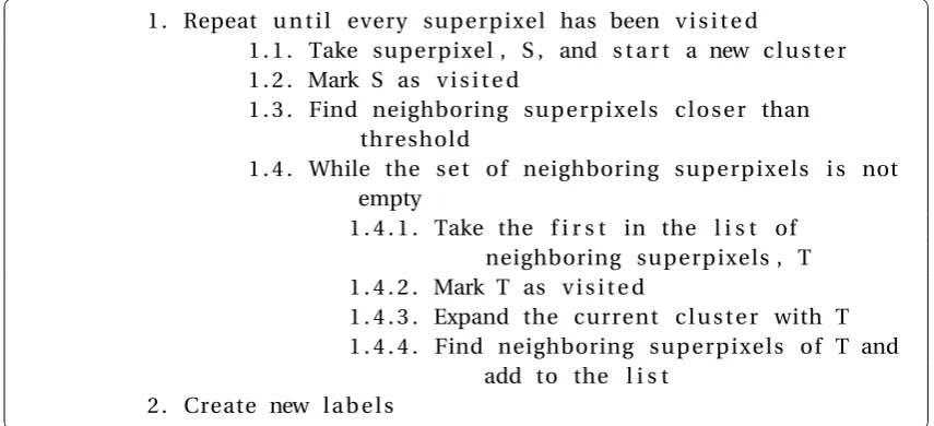
DBSCAN is effectively a region growing technique that can best be explained by referring to the pseudo code below:
1 . Repeat u n t i l every superpixel has been v i s i t e d
1 . 1 . Take superpixel , S , and s t a r t a new c l u s t e r 1 . 2 . Mark S as v i s i t e d
1 . 3 . Find neighboring superpixels c l o s e r than threshold
1 . 4 . While the s e t of neighboring superpixels i s not empty
1 . 4 . 1 . Take the f i r s t in the l i s t of neighboring superpixels , T 1 . 4 . 2 . Mark T as v i s i t e d
1 . 4 . 3 . Expand the current c l u s t e r with T 1 . 4 . 4 . Find neighboring superpixels of T and
add to the l i s t 2 . Create new l a b e l s
Basically the algorithm starts by taking a superpixel, marking it as visited and starting a cluster with it. Next it finds all the neighboring superpixels with a distance smaller than the threshold. It visits this list of neighboring superpixels, adds them to the cluster and marks them as visited, then expands the list of neighbors with the neighboring superpixels of those, again, within a distance smaller than the threshold. So the list of neighbors is being expanded whenever there are connected superpixels being found within a distance smaller than the threshold. This pro-cess continues until the list of neighboring superpixels is exhausted. At this point a new cluster is started with a superpixel that has not been visited by the algorithm yet.
Because in this process, the label the newly made cluster is assigned is simply the label of the superpixel the cluster has been started with, the labels will not be sequential anymore. There-fore, the last step is a renumbering of all the clusters so their labels are again a sequential list
[image:30.595.71.499.332.527.2][1, . . . ,N] whereN is the total number of clusters.
example at the top of the round tumor area on the bottom, stroma is taken with the tumor in the last two images.
1299 superpixels 823 superpixels
756 superpixels 695 superpixels 640 superpixels 597 superpixels
Figuur 4.4:Left to right, top to bottom: The original image, the original overlaid with the superpixels and 5 images after using the DBSCAN
5 Results
In the previous chapter the SLIC algorithm was explained in detail, a few intermediate results were shown as were the workings of the DBSCAN algorithm. But to be able to say something about how well the algorithm as a whole performs, a couple things are needed.
First a ground truth is needed. In the case of the H&E stained pathology images the ground truth was provided by someone with expertise in the area. An example of an H&E stained pa-thology image with its ground truth can be seen in columns (a) and (b) of Figure 5.2. The ground truth shows a partition of the original image in a black and a gray section. The black section represents tumor and the gray section stroma.
The second thing that is needed is a clear formulation of the requirements the superpixels have to meet. In other words, properties by which to indicate how good a set of superpixels is. Since the goal of the pre-processing method is to reduce the effective number of pixels without losing the information present in the image, the first property is readily stated: size. The superpixels have to be as large as possible. The larger the superpixels, the easier for the MRF-based seg-mentation algorithm. Of course, there is no size for the superpixels to refer to. This depends for example on the image size, but also on the features present in the image. The first row in Figure 5.2 shows an H&E stained pathology image with a fairly clear distinction between tumor and stroma so the superpixels can be larger in this case than when tumor and stroma are more intertwined (see for example the last two rows in Figure 5.2). However, if two sets of superpixels for the same image are compared and the accuracy is comparable, then the set with the largest superpixels is preferable. This leads to the second property: accuracy. The accuracy of a set of superpixels is a measure of how well the boundaries of the superpixels agree with the boun-daries of the ground truth. This is also called boundary recall. Since even segmenting H&E stained pathology images by hand by an expert pathologist is prone to error, two limits were chosen. The lower limit was set to three and the upper limit to six. The lower limit says that if a superpixel boundary falls within three pixels of the ground truth boundary it is still counted as correct. If it is further away but falls within six pixels from the ground truth boundary it is still acceptable. Superpixel boundaries further away are counted as wrong. There is one exception
to this. Even if a superpixel boundary pixel doesnâ ˘A ´Zt fall within three pixels from the ground
truth boundary, it can still be counted as correct if that pixel falls within a white area. As can be seen on the original H&E stained images (column (a) in Figure 5.2), there can be quite a lot of white in the image. This white matter is neither tumor nor stroma so if a superpixel boundary cuts through this white matter it does not influence the accuracy of the set of superpixels. Be-cause measuring the accuracy this way is not exact and to still be able to distinguish between sets of superpixels with comparable accuracy, the average distance (in number of pixels) the superpixel boundaries are away from the ground truth boundaries is also calculated for the boundary pixels classified as acceptable.
5.1 Measurement algorithm
To determine which and how many boundary pixels from the ground truth can be classified as correct, acceptable and wrong, two edge maps are created: one from the ground truth and one from the superpixels generated by the SLIC algorithm. Next a distance transform is ap-plied to the superpixel edge map. The distance transform determines for every pixel that is not a boundary pixel how far away from the closest boundary it is located. Lastly, as explained earlier, pixels are also classified as correct if they are further away from the ground truth
boun-daries thanLBbut fall within the white matter. Therefore, an image indicating the white matter
Figuur 5.1:Left to right: The ground truth edge map, white matter connected to the ground truth boundaries, superpixel edge map and the
distance transform from the superpixel edge map
on the original H&E stained image. It is assumed that pixels with a luminance value larger than 0.7 times the maximum luminance value found in the image are white matter. The distance transform of the superpixel edge map is shown in color, where a darker color indicates a closer proximity to a border, for clarity.
LetAbe the set of pixels belonging to the boundaries of the ground truth,Bthe set of pixels
be-longing to the boundaries of the superpixels anddB(A)≤na function that returns the ground
truth boundary pixels within a distancenfrom a superpixel boundary. In the case that pixels
within a distance>LBand≤U Bpixels from the ground truth border are classified as
accepta-ble, this can now be expressed mathematically as follows:
Aaccept abl e={A|dB(A)>LB∧dB(A)≤U B} (5.1)
WhereLBandU B are the lower and upper bounds for accepted distances respectively. The
percentagePaccept abl eof correctly classified pixels can be expressed as:
Paccep t abl e=
|Aaccep t abl e|
|A| (5.2)
Similar equations hold for the pixels classified as wrong. The equation for correctly classified pixels has an extra condition that even when pixels are further away from the ground trust
boundaries thanLBpixels, they can still be classified as correct if they are in the white matter
connected to the boundary. IfCis the set of pixels consisting of white matter connected to the
ground truth boundary then the equation becomes:
Acor r ec t={A|dB(A)≤LB∨C(A)} (5.3)
When interested in the average distancedaver ag e that pixels classified as acceptable are from
the ground truth boundaries, this can be calculated as follows:
daver ag e= U B
X
n=LB+1
|Aaver ag e(n)|
|A| n (5.4)
Aaver ag e(n) is a function that returns the set of pixels classified as average at distancenfrom
the ground truth boundaries. The results in column (d) in Figure 5.2 where obtained in this way and show a bar chart indicating which portion of the ground truth boundaries was classified as correct, acceptable and wrong for an increasing number of initial superpixels.
1299 superpixels
5001000 1500 2000 2500 3000 3500 4000 4500 5000 0 10 20 30 40 50 60 70 80 90 100
Number of initial superpixels
Boundary recall in %
Correct Acceptable Wrong
1216 superpixels
5001000 1500 2000 2500 3000 3500 4000 4500 5000 0 10 20 30 40 50 60 70 80 90 100
Number of initial superpixels
Boundary recall in %
Correct Acceptable Wrong
1230 superpixels
5001000 1500 2000 2500 3000 3500 4000 4500 5000 0 10 20 30 40 50 60 70 80 90 100
Number of initial superpixels
Boundary recall in %
Correct Acceptable Wrong
1204 superpixels
5001000 1500 2000 2500 3000 3500 4000 4500 5000 0 10 20 30 40 50 60 70 80 90 100
Number of initial superpixels
Boundary recall in %
Correct Acceptable Wrong
1798 superpixels
5001000 1500 2000 2500 3000 3500 4000 4500 5000 0 10 20 30 40 50 60 70 80 90 100
Number of initial superpixels
Boundary recall in %
Correct Acceptable Wrong (a) (b) 1942 superpixels (c)
5001000 1500 2000 2500 3000 3500 4000 4500 5000 0 10 20 30 40 50 60 70 80 90 100
Number of initial superpixels
Boundary recall in %
Correct Acceptable Wrong
(d)
Figuur 5.2:(a) Original H&E stained image (b) The ground truth (c) Superpixels overlaid on the original image (d) Bar chart of boundary recall