Rational maps with clustering and the mating of polynomials

(1)

University of Warwick institutional repository: http://go.warwick.ac.uk/wrap

A Thesis Submitted for the Degree of PhD at the University of Warwick

http://go.warwick.ac.uk/wrap/35776

This thesis is made available online and is protected by original copyright.

Please scroll down to view the document itself.

(2)

AUTHOR:_{Thomas Joseph Sharland} DEGREE: _Ph.D.

TITLE:_{Rational Maps with Clustering and the Mating of Polynomials} DATE OF DEPOSIT: _{. . . .}

I agree that this thesis shall be available in accordance with the regulations governing the University of Warwick theses.

I agree that the summary of this thesis may be submitted for publication. I agree that the thesis may be photocopied (single copies for study purposes only).

Theses with no restriction on photocopying will also be made available to the British Library for microfilming. The British Library may supply copies to individuals or libraries. subject to a statement from them that the copy is supplied for non-publishing purposes. All copies supplied by the British Library will carry the following statement:

“Attention is drawn to the fact that the copyright of this thesis rests with its author. This copy of the thesis has been supplied on the condition that anyone who consults it is understood to recognise that its copyright rests with its author and that no quotation from the thesis and no information derived from it may be published without the author’s written consent.”

AUTHOR’S SIGNATURE: _{. . . .}

USER’S DECLARATION

1. I undertake not to quote or make use of any information from this thesis without making acknowledgement to the author.

2. I further undertake to allow no-one else to use this thesis while it is in my care.

DATE SIGNATURE ADDRESS

. . . .

(3)

M A

E

G

NS I

T A T MOLEM

U N

IV

ER

SITAS WARWICEN

SIS

Rational Maps with Clustering and the Mating of

Polynomials

by

Thomas Joseph Sharland

Thesis

Submitted to The University of Warwick

for the degree of

Doctor of Philosophy

Mathematics

(4)

List of Figures

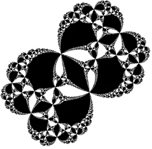
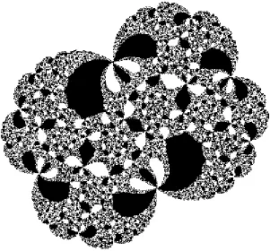
1.1 An example of a map with a cluster point. . . 3

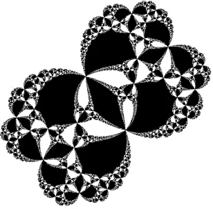
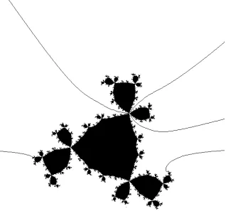
1.2 An example of a map with a period 2 cluster cycle. . . 5

1.3 A “period 4 rabbit”, or 4-rabbit, Julia set with some equipotential curves. . . 12

1.4 The Douady’s rabbit Julia set (z 7→ z2_{+ (}₋₀_.₁₂₂₅_{. . .}_{+ 0}_.₇₄₄₈_{. . . i}₎

with external rays of the formθ=p/7, 0≤p≤6 . . . 13

1.5 The Mandelbrot Set,M . . . 16

1.6 An example of parameter rays inM. The region bounded by the rays is the (22/63,25/63)-wake. . . 20

1.7 The degree 3 Multibrot set. . . 33

1.8 A degree 3 rabbit (corresponding to the parameter rays 1/26 and 3/26) and the external rays landing on the two β-fixed points and theα-fixed point. . . 34

2.1 The graph which is topologically equivalent to [α1]. . . 50

2.2 A schematic diagram showing the ray class [α1]. E is the equator. . 51

3.1 An example of a map with a cluster point. . . 57

3.2 A “double rabbit” and some rays landing on the period 2 cycle. . . . 58

3.3 An n-rabbit and some rays landing on the α-fixed point. . . 59

4.1 The “V-shaped” curve Λ1. . . 66

4.2 The multicurve Γ. . . 67

4.3 The curves ˆΛ0 (continuous line) and ˆΛ0 (dashed line). . . 67

4.4 The curves ˆγ0 and ˆγ01 (dashed line) in the cased= 2. . . 68

4.5 Construction of the mapψ in Lemma 4.3.8. . . 81

(9)

4.7 The (isotopy class of the) equator in the fixed cluster point case. . . 89 4.8 The pre-image of the equator from Figure 4.7. . . 90

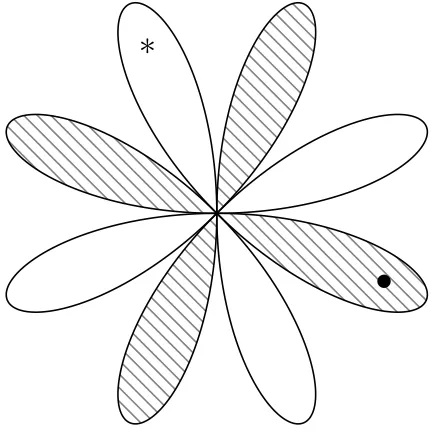
5.1 A cluster with critical displacement 5. We use ∗ to represent the critical point c1 and the dot to represent the critical value which is

the image of the second critical point c2. The shading is used to

differentiate between components for the orbit ofc1 andc2. . . 99

5.2 The double rabbit component and secondary map component of pe-riod 8, rotation number 1/4 case. . . 101 5.3 The double rabbit, corresponding to the parameter rays in Figure 5.2

with the external rays landing on the period 2 orbit and on theα-fixed point. . . 103 5.4 The secondary map that belongs to the wake of the limb containing

the double rabbit in Figure 5.3, with the external rays landing on the period 2 orbit and the α-fixed point. Also included are the rays landing at the root points of the critical orbit Fatou components. . . 104 5.5 Diagram for proof of proposition 5.2.17. . . 112 5.6 Hubbard tree for 1→22/5→9→10. . . 113

5.7 The rays landing at the period two point and critical value component of the mapg. . . 114 5.8 The case where the branch containingr contains the ray of angle φ. 115 5.9 How the ray class is formed near the critical value component of g.

Rh₋₍_θ₊₂₎ must be an endpoint. . . 116 5.10 Whencj andckare endpoints of the Hubbard tree, the cyclic ordering

of the rays is maintained. . . 120 5.11 Ifcj is not an endpoint, then the cyclic ordering of the two ray orbits

is changed. . . 121 5.12 The map Ψ. . . 125 5.13 Diagram for the proof of Lemma 5.3.8. The dashed lines represent

the modification that comes about if we add a Dehn twist in the range before pulling back underG. Compare with Figure 5.14. . . 129 5.14 The “modified” diagram from Figure 5.14, with the new regions

B1, . . . ,Bdlabelled. . . 130

(10)

5.17 A curve isotopic to the equatorE in Figure 5.15. This is isotopic rel

PF to a tubular neighbourhood of the Hubbard tree of h. . . 136

A.1 Period 5, Rotation number 1/5 . . . 143

B.1 Period 4, Rotation number 1/2 . . . 166

(11)

C.1 Hubbard tree for 1→3, rotation number 1 . . . 195

C.2 Hubbard tree for 1→2→3, c.d = 3 . . . 195

C.5 Hubbard tree for 1→2→3→4, c.d = 5 . . . 197

C.17 Hubbard tree for 1→3→4→5→6, c.d = 7 . . . 203

C.18 Hubbard tree for 1→2→3→4→5→ 6, c.d = 9 . . . 203

C.24 Hubbard tree for 1→2→3→4→5→ 6→7, c.d = 11 . . . 206

(12)

D.1 Hubbard tree for 1→2→4, rotation number 1 . . . 213

D.2 Hubbard tree for 1→2→3→4, rotation number 1 . . . 213

D.3 Hubbard tree for 11/3 →3→4,c.d=1. . . 214

D.4 Hubbard tree for 1₂_/₃ →3→4,c.d=3. . . 214

D.7 Hubbard tree for 1→5→6,c.d=1. . . 216

D.8 Hubbard tree for 1→3→4→6,c.d=3. . . 216

D.9 Hubbard tree for 1→3→5→7→8,c.d=5. . . 217

D.21 Hubbard tree for 1→3→4→6→8→ 10,c.d=7. . . 225

(13)

D.35 Hubbard tree for 1→5→6→8→10→12,c.d=7. . . 233

D.36 Hubbard tree for 1→3→4→6→8→ 10→12,c.d=9. . . 233

D.37 Hubbard tree for 1→3→5→7→9→ 11→12,c.d=11. . . 234

D.44 Hubbard tree for 1→5→6→8→10→12→14,c.d=9. . . 239

D.45 Hubbard tree for 1→3→4→6→8→ 10→12→14,c.d=11. . . . 240

D.52 Hubbard tree for 1→3→4→6→9→ 11→12→14,c.d=7. . . 245

D.59 Hubbard tree for 1→3→4→7→9→ 12→13→14,c.d=3. . . 249

(14)

D.63 Hubbard tree for 1→3→6→7→9→ 10→14,c.d=11. . . 251 D.64 Hubbard tree for 1→3→6→7→10→11→13→14,c.d=13. . . 252

E.1 The Julia set of the map f1 with the external rays landing on the

period two orbit that becomes the cluster cycle. . . 254 E.2 The Julia set forf2, the map which mates with f1 to create a period

2 cycle. Note the external rays that have been drawn land at non-principal root points of the Fatou components. . . 255

(15)

Acknowledgments

First of all I would like to thank my parents, Cheryl Sharland and Andrew Sharland,

for all the support they have shown me and for always lending a sympathetic ear

whenever I need it. I am very grateful for the many sacrifices they have both made

in order for me to have the opportunity to study for a PhD.

I would also like to thank my supervisor, Dr Adam Epstein whose patience

and guidance has been extremely helpful during the course of this research. His

willingness to discuss not just complex dynamics but also many other area of

math-ematics, as well as provide encouragement throughout the course of my research

has been invaluable. I would also like to thank my examiners, Professor Anthony

Manning and Professor Mary Rees, for agreeing to read the thesis and for providing

a number of useful corrections and suggestions for improving the final document.

Furthermore I would like to thank all the people in the Mathematics Institute

at the University of Warwick that have helped me in any way, whether by useful

discussions on the mathematics or by aiding my sanity by providing welcome and

interesting conversation when my mind required rest. In particular I would like

to thank Professor Anthony Manning who provided a number of useful discussions

and in particular pointed me towards the power of symbolic dynamics in describing

quadratic polynomials. I would like to thank James for his good humour and many

enjoyable conversations. Finally, a special mention to Ay¸se’m for her love and

support.

This research was funded by a grant from the Engineering and Physical

(16)

Declarations

I declare that this thesis and the work presented in it are my own and represent my

own original research. Wherever contributions of others are included, I have

endeav-oured to ensure that this is stated clearly and attributed with explicit references.

No part of this thesis has been submitted for a degree or any other qualification at

(17)

Abstract

The main focus of this thesis is the study of a special class of bicritical rational maps

of the Riemann sphere. This special property will be called clustering; which

infor-mally is when a subcollection of the immediate basins of the two (super-)attracting

periodic orbits meet at a periodic pointp, and so the basins of the attracting

peri-odic orbits are clustered around the points on the orbit ofp. Restricting ourselves

to the cases wherepis fixed or of period 2, we investigate the structure of such maps

combinatorially; in particular showing a very simple collection ofcombinatorial data

is enough to define a rational map uniquely in the sense of Thurston. We also use

the language of symbolic dynamics to investigate pairs (f, g) of polynomials such

thatf ⊥⊥ g has a fixed or period two cluster point. We find that that the internal

addresses of such maps follow very definite patterns which can be shown to hold in

(18)

Chapter 1

Introduction

1.1 Overview

Complex dynamics emergence as a popular subject for mathematical research came about as a result of the rediscovery of the early 20th Century works of Fatou [Fat19, Fat20] and Julia [Jul18]. After a comparably quiet period, the subject was given a new life in the 1980s. Perhaps the most notable contributions were supplied by A. Douady and J. Hubbard, whose “Orsay lecture notes” [DH84, DH85] provide a number of enlightening and amazing results about the behaviour of such systems. A lot of the work has been motivated by the many pictures of the various objects found in this topic, not least the Mandelbrot set.

The focus of this thesis is the study of rational maps which have a cluster cycle. Clustering is a property found in some bicritical rational maps - that is, rational maps with precisely two critical points. We define clustering informally below and more formally in Chapter 3. One way of constructing maps with this property is by mating together monic unicritical polynomials (polynomials with only one finite critical point) of the formzd₊_c_{. We outline the general structure of}

the thesis, and emphasise some of the main results found during the research. We will use some terms and notions which are defined more formally in the main body of the thesis, but we will endeavour to outline these notions in this overview.

(19)

the properties we require for the definition of a mating (as defined in the thesis) to make sense. We also introduce some notions from symbolic dynamics - for example, the internal address - since we will be making use of this theory throughout the thesis.

Let ΩF be the set of critical points of a map. Recall that a map is

postcriti-cally finite if the set

PF :=

[

n>0

F◦n(ΩF)

is a finite set. PF is called the postcritical set of the map F. In Chapter 2, we

focus on the study of postcritically finite branched self-coverings of a topological sphere. A mapf:X → Y is called a branched covering if there exists a finite set

Z ⊂Y such that the restricted mapf:X\f−1(Z)→Y \Z is a covering map. The branched coverings in this chapter will, in the main, be constructed by “mating” two degreed(the degree of a branched covering is the number of pre-images - including multiplicity - of each point in the image) monic polynomials f1 and f2. There are

actually a number of different definitions of mating, and we endeavour in Chapter 2 to outline the differences and connections between them. We also discuss some properties of matings that will be useful in later chapters.

One of the most important results in the theory of branched coverings is the notion ofThurston equivalence. It gives a condition for checking whether or not two branched coverings are, in some sense, the same. Furthermore,Thurston’s Theorem

realises the full power of this equivalence, by showing that each equivalence class contains only one rational map, up to M¨obius transformation. We will find two uses of the theorem in the thesis. Firstly, it will allows us to discuss, in general, when a branched self-covering of the sphere constructed by a mating is equivalent to a rational map. Secondly, we will use it in the chapters on clustering to discuss the equivalence of rational maps which have clusters of the same period; more on this later.

(20)

[image:20.595.168.476.175.478.2]

chapter the notion of combinatorial data of a cluster, which will be made up of a pair (ρ, δ), where ρ is the combinatorial rotation number and δ will be called the critical displacement.

Figure 1.1: An example of a map with a cluster point.

(21)

The other focus of this chapter is on the properties of polynomialsf1 andf2,

such that the mating F ∼=f1 ⊥⊥f2 has a fixed cluster cycle. We will show that we

able to be quite specific about one of the maps: precisely one of them has to be an

n-rabbit; that is, a map which belongs to a hyperbolic component that bifurcates off of the unique period one component in parameter space. This is unsurprising; when one looks at the Julia set of a map with a fixed cluster cycle, one can often “see” the Julia set of ann-rabbit inside it. For example, one notices the shape of the rabbit polynomial in Figure 1.1. The properties of the “complementary” map - the

fiwhich is not ann-rabbit - are a little more difficult to study. However, we are still

able to carry out a classification to some extent. To do this, we take advantage of the fact that the combinatorial rotation number of theα-fixed point of then-rabbit in the mating will force an ordering of the angles of the rays landing at the root point of the critical orbit Fatou components of the complementary map. We then show that the maps that have the “correct” angular ordering are precisely those that create a rational map with a fixed cluster point when mated with ann-rabbit. Combined with the result on Thurston equivalence, we get the following theorem.

Theorem 4.0.3. Suppose that F is a bicritical rational map with a fixed clus-ter point and the combinatorial rotation number isp/n. ThenF is the mating of an

n-rabbit with angled internal address 1p/n →n and another map h. In the degree 2 case, h has an associated angle with angular rotation number (n−p)/n.

Finally the case where the cluster is of period 2 is discussed in Chapter 5. This case, unsurprisingly, is more complicated than when the cluster is fixed, and a num-ber of the results found were perhapsa priori unexpected after one has considered only the fixed cluster case. In this chapter we will compare and contrast the two cases. In Appendix F we will also discuss some examples with clusters of higher period, showing why an increase in period beyond two creates a number of com-plications that makes studying this phenomenon much more involved. Again, the main theorem of this chapter (Theorem 5.3.2) shows that the combinatorial data is once again enough to classify the rational map in the sense of Thurston, at least in the quadratic case. We also discuss the difficulties of extending this result to the general case for degreedbicritical maps with a period two cluster cycle.

As with the previous chapter, we also investigate the properties of f1 and

f2 under the assumption that F ∼= f1 ⊥⊥ f2 is a rational map with a period two

(22)

[image:22.595.173.474.330.610.2]

Mandelbrot set. The results in the one cluster case may lead us to conjecture that the map belonging to the (1/3,2/3)-limb would have to be a map belonging to a hyperbolic component which bifurcates off of the period two component of the Mandelbrot set. However, in the two cluster case, we are no longer able to make out the shape of these “double rabbits” (maps which belong to hyperbolic components which bifurcate off of the period two component of the Mandelbrot set) in the Julia sets of these maps (see Figure 1.2). Indeed, we will show it is no longer true that one of the maps has to belong to a bifurcation component. There is a secondary component of period 2n, which belongs to the limb of the Mandelbrot set beyond these bifurcation components of 2n. It turns out that, in certain cases, this secondary map can be mated with another polynomial to create a map with a period two cluster cycle.

Figure 1.2: An example of a map with a period 2 cluster cycle.

(23)

is a double rabbit, we can ask what we can say about the properties of the maph

if we know thathmates with a double rabbit to form a rational map with a period two cluster cycle. A similar technique as that used in the fixed cluster case again yields a necessary condition on the complementary maps. Furthermore, we can ask what conditions are needed on the complementary maphin order for this secondary map to be able to create a rational map with a period two cluster cycle when mated withh? Again, we discuss this problem combinatorially, and see that there is a very simple restriction on the combinatorial data of the rational maps constructed in this way.

The other aspect of this thesis is the study of progressions of internal ad-dresses and Hubbard trees. For example, in the fixed cluster case, we know from the work of Chapter 4 that one of the maps is ann-rabbit. Therefore, most of the study into the properties of the maps in the matings that create maps with fixed cluster cycles is into the properties of the complementary map. In the appendices, we have given the internal addresses of these complementary maps for given com-binatorial data. It turns out that there are a number of progressions which seem to follow some sort of set pattern. We prove these progressions in simple cases -hold for arbitrarily large periods. The author is confident that more patterns in the progressions could be found in more complicated cases.

As well as cataloguing these complementary maps, the appendices also in-clude the Hubbard trees of the complementary maps in cases of low degree. Though not necessarily vital to the exposition, these trees give the raw data that was used in the formulation of a number of the results and again, in some cases, the reader will see that in some sense there are patterns followed by the Hubbard trees as the period increases, at least in simple cases. Finally, we include an appendix discussing the increased complexity found as the period of the clusters goes from two to three, and towards even higher periods. There is very little formal discussion in this final appendix, but conjectures are made as to what the author expects to happen for higher periods.

A standard reference for complex analysis may be useful. For this purpose, the author heartily recommends either [Ahl78] or [Con78].

1.2 Preliminaries

(24)

Riemann sphere and denote it by C. When we wish to use the complex numbers with the circle of directions at infinity, we will writeCb = C∪ {∞ ·e2πis : s∈ R}; this space is homeomorphic to the closed unit disk.

1.2.1 Notation and terminology

If, for some n ≥ 1 and w ∈ C we have f◦n(w) = w, then we say w is a periodic

point. If, furthermore,nis the smallest such integer satisfying this property, we say the period ofw isn. If whas period 1 we call it afixed point of f.

Now supposewis a periodic point of period n. Then themultiplier,µ, of f

at wis defined to be

µ= (f◦n)′(w) =

n_Y−1

k=0

f′(f◦k(w)).

We can now classify periodic points according to the modulus of their multipliers.

Definition 1.2.1 (Classification of periodic points). A periodic point is called

• superattracting if µ= 0.

• attracting if |µ|<1.

• rationally indifferent (or parabolic) if µ=e2πiθ,θ∈Q.

• irrationally indifferent if µ=e2πiθ_, _θ_∈_R_\_Q_.

• repelling if |µ|>1.

It is reassuring to note that the definitions given above (using the multiplier to describe the behaviour of a periodic point) agree with the usual dynamical (or topological) definition of attracting. That is to say, a fixed pointpis (topologically) attracting if there exists a neighbourhoodU of p such that the iterates f◦n are all defined in U and they converge to the constant map z7→ p. A similar equivalence holds for repelling points.

Given any pointz, theorbit of z is defined as the set

O(z0) ={z, f(z), . . . , f◦n(z), . . .}.

Now, given an attracting cycle (we use the terms “cycle” and “periodic orbit” interchangeably) a natural question to ask is, which points are attracted to it? We define thebasin of attraction of an attracting cycleOof periodnto be the open set

A={z:f◦kn₍_z₎ _→_p _{for some}_p_{∈ O}}_{. The}_{immediate basin} _{(of attraction) is the}

(25)

Definition 1.2.2. Let z∈C. If in any neighbourhood of z,f is not a homeomor-phism onto its image, then we sayz is a critical point off. In other words, z is a critical point precisely when the local degree off at z is greater than 1.

Indeed, in a neighbourhood of a critical point, it is possible to conjugate the map to adth power mapz7→zd_{, and so a neighbourhood of the critical point maps}

in ad-to-1 way onto its image. Conversely, if z is not a critical point then there is a neighbourhood ofzon which f is a homeomorphism.

Note that in the case wheref(z) =zd₊_c_{, 0 is the only finite critical point}

(∞ is a superattracting fixed point) and the critical value isc.

1.2.2 Fatou and Julia Theory

We now outline the basic definitions and results needed in the rest of this thesis. First of all we restate a standard definition from complex analysis. A good refer-ence for background material required from complex analysis can be found in, for example [Ahl78] or [Con78]. We will generally avoid stating well-known results from complex analysis, except where we deem it relevant or if the statement is required for emphasis. In what follows, we assume that the functionf is rational.

Definition 1.2.3 (Normal Family of Functions). Let U ⊂ C. A family F _of

holomorphic functions f : U → C is normal in U if each sequence in F _{has a}

subsequence which converges to a holomorphic function g:U →C.

Note that the functiong does not have to be in F_{. In some sense, normal}

families of functions are “well-behaved”. Indeed, if we take F _⊂ _Hol(_U,_C_{) then}

a family is normal precisely when it has compact closure in the function space Hol(U,C).

Definition 1.2.4. Let f: C → C be a rational map on the Riemann sphere, of degree at least 2. Consider the family F _:= _{f◦n _: _n _∈ _N_}. _{We now split the}

Riemann sphere into two disjoint sets. Let z∈ C. If there exists a neighbourhood

U ∋z so that the familyF _{is normal in}_U_{, then we say} _z _{belongs to the}_{Fatou set}

off,F(f). Ifzdoes not belong to the Fatou set, then we say it belongs to theJulia set of f, which we denote byJ(f).

(26)

components which contain points on the critical orbit will play an important role in the discussion of clustering, and these are given more attention in Definition 3.1.1. At certain points, especially when we are dealing with the dynamics of polynomials, it will be important to consider the set of points with bounded orbits. This set is called the filled Julia set, K(f). Note that we have ∂K(f) = J(f), and the components of K(f)\J(f) are the bounded Fatou components. Alternatively, we can defineK(f) as

K(f) : ={z:f◦n(z)9∞}

The setsF(f),J(f) and K(f) are all completely invariant under iteration off.

Remark 1.2.5. The definition given above is the original one given by Fatou [Fat19, Fat20]. Gaston Julia gave a different but equivalent definition: the Julia set is the closure of the set of repelling periodic points [Jul18] . The proof of this equivalence can be found in [Mil06].

Remark 1.2.6. It can easily be seen that F(f) is an open set in C. It therefore follows that J(f) is a closed set. Indeed, under the assumption that f is a non-linear polynomial, J(f) is a closed, compact set with no isolated points. Similarly,

K(f) is closed.

We find that the behaviour of the critical points of a map are very important in studying the general behaviour of the map.

Theorem 1.2.7 ([Mil06], Theorem 8.6). Suppose f is a rational map of degree

d ≥ 2. Then the immediate basin A0 of every attracting periodic orbit of f must contain a critical point.

We have the following very important theorem. The (sharp) bound was found first by Shishikura [Shi87] and a refinement using a different method was given by Epstein [Eps99].

Theorem 1.2.8. A rational map can have only a finite number of attracting or indifferent cycles. Indeed, if the degree of the rational map is d > 1, then the number of attracting or indifferent cycles is at most 2d−2.

(27)

1.3 External rays

An important aspect of dynamical systems is the ability to conjugate the dynamics of two systems under a change of variable map. In this section, we will use a conjugacy between the dynamics of f on C\K(f) and the map z 7→ zd _on _C_\_D

to construct external rays. These rays are an important component in defining the notion of mating of polynomials in Chapter 2.

We begin with a theorem due to B¨ottcher [B¨ot04]. The statement below is as found in [Mil06], Theorem 9.1.

Theorem 1.3.1 (B¨ottcher’s theorem). Let f be a holomorphic germ of the form

f(z) =adzd+ad+1zd+1· · ·

withd≥2andad6= 0. Then there is a holomorphic change of co-ordinates w=φ(z) with the properties that

• φ(0) = 0,

• φ conjugates f to the map w7→wd _{in a neighbourhood of 0.}

The map φ is also unique up to multiplication by an (d−1)st root of unity. In particular, it is unique in the case where the local degree is 2.

Now suppose that we have a monic degreed(d≥2) polynomial f:C→C, given by

f(z) =zd+ad−1zd−1+· · ·+a1z+a0.

By considering the local behaviour at infinity (by using the change of co-ordinates

z7→1/z), we see that this map has a superattracting fixed point at infinity, and so we can apply B¨ottcher’s theorem there.

The following appears as Theorem 9.5 in [Mil06].

Theorem 1.3.2. Let f be a monic polynomial of degree d≥2. If the filled Julia set

K = K(f) contains all of the finite critical points of f, then both K and J =∂K

are connected and the complement of K is conformally isomorphic to the exterior of the closed diskD under an isomorphism

ˆ

φ:C\K →C\D,

(28)

many connected components. Moreover, the map φˆ is asymptotic to the identity at infinity.

From the function ˆφ defined above (which we relabel with φ) we get the

Green’s function forK, which is defined as

G(z) = (

log|φ(z)|, z ∈C\K;

0, z∈K.

Gis strictly positive and harmonic onC\K and continuous everywhere. Trivially, it is asymptotic to log|φ(z)|at infinity and since φconjugates f to the mapw7→wd_, Gsatisfies the identity G(f(z)) =dG(z).

Let ρ > 0. Then the pre-image G−1₍_ρ_{) =} _{z _∈ _C _: _G₍_z_{) =} _ρ} _{is a closed}

curve which we call theequipotential curve of orderρ (Figure 1.3). Perhaps of more importance than these equipotential curves (at least in terms of our applications) are their orthogonal trajectories, known asexternal rays.

Definition 1.3.3. The external ray of angleθ for a mapf,Rf_θ, is defined as

Rf_θ: ={z∈C: arg(φ(z)) = 2πθ}

whereφis the B¨ottcher co-ordinate at ∞ from Theorem 1.3.1.

We will sometimes omit the functionf from the notation if it is arbitrary or clear in the context.

It should be noted that the external rays are the pre-images of points of the form re2πiθ for r > 1. A sensible question is therefore to ask: when does limrց1φ−1(re2πiθ) exist? In fact, the limit exists for all rational θ and when the

Julia set is locally connected then it is known that this limit exists for all θ (see Proposition 1.3.7 below). It is clear from the definition that if limrց1φ−1(re2πiθ) =z

thenz∈∂K(f) =J(f); we say the external rayRf_θ lands at z.

Theorem 1.3.4. Assume thatK(f) is connected. Then every periodic external ray lands at a periodic point which is either repelling or parabolic. Conversely, every repelling or parabolic periodic pointz0 is the landing point of (at least) one external ray, which itself must be periodic, with period divisible by the period ofz0.

In order to say more than the above, we need to introduce a further condition, that of local connectivity.

(29)

Figure 1.3: A “period 4 rabbit”, or 4-rabbit, Julia set with some equipotential curves.

The following result was originally proved in [Car13], and is stated as found in [Pom92].

Theorem 1.3.6 (Carath´eodory’s theorem). Let f map D conformally onto the bounded domainG. Then the following three conditions are equivalent:

1. f has a continuous injective extension to D;

2. ∂G is a Jordan curve;

3. ∂G is locally connected and has no cut points.

In our setting, local connectivity is what is required to ensure that all the rays will land.

(30)

Figure 1.4: The Douady’s rabbit Julia set (z7→z2_{+ (}₋₀_.₁₂₂₅_{. . .}_{+ 0}_.₇₄₄₈_{. . . i}_{) with}

external rays of the formθ=p/7, 0≤p≤6

1. The Julia set, J(f) is locally connected.

2. The filled Julia set K(f) is locally connected.

3. For every θ, the external ray Rf_θ lands at a point (which we denote by γf₍_θ₎_, or sometimes γ(θ) if f is clear in the context) on the Julia set. This point

γf(t) depends continuously on the angleθ.

4. Furthermore, the inverse B¨ottcher mapφ−1 can be extended continuously over the boundary of ∂D, and φ−1₍_e2πiθ_{) =}_γ₍_θ₎ _{for all}_θ_.

In this thesis, we will be assuming that the Julia set is connected, and so we can apply the above proposition. Suppose that the conditions in the above proposition are satisfied. Then the newly defined mapγ:R/Z→J(f) is called the

(31)

the circle R/Z onto the Julia set J(f) and satisfies

γ(dθ) =f(γ(θ)), (1.1)

wheredis the degree of the polynomialf. The following is well-known, for example see [Mil00b].

Proposition 1.3.8. Suppose the external rayRf_θ lands atz∈J(f). ThenRf_dθ lands at f(z). Furthermore, suppose that there are at least three rays Rf_θ

1, R

f

θ2, . . . , R

f θk landing at some z6= 0, then the cyclic ordering of the angles θj on the circle is the same as the cyclic ordering of the angles dθj on the circle.

1.3.1 Properties of External Rays

The following two results tell us about the behaviour of external rays with respect to points in the Julia set. Again they can be found in [Mil00b], and are general folklore.

Proposition 1.3.9. Assume K(f) is connected. If a periodic ray lands at z0, then only finitely many rays can land atz0 and all rays landing atz0 are periodic of the same period. In particular, if the period of each ray is p, the denominator of the angle of the rays is2p₋₁_.

In general, we will be dealing with hyperbolic polynomials, which means there are no parabolic cycles. In that case, the previous theorem says that all periodic rays land on repelling periodic points.

We now discuss some of the elementary properties of the external rays. First we take advantage of (1.1) to mark some special points onJ(f).

Definition 1.3.10. The pointγ(0), the landing point of the rayR0is a fixed point of

f, called theβ-fixed point off, orβ for short. In the case of quadratic polynomials, the other (finite) fixed point is called the α-fixed point. If fc(z) = zd+c, then

the raysR_k/f ₍_d₋₁₎ (k= 0,1, . . . , d−2) land at fixed points. We will label the point

γf₍_k/₍_d₋_{1)) by} _β

k in this case. If there is another finite fixed point of the mapfc,

then it will be called theα-fixed point.

For example, theα-fixed point for the Julia set in Figure 1.4 is the landing point of the external rays of angle 1/7, 2/7 and 4/7. Theβ-fixed point is the landing point of the ray of angle 0 = 0/7.

(32)

βkfixed points and theα-fixed point, these make up all the possible fixed points for

the polynomial fc. We restrict our attention to degree 2 below, but similar results

can be proved in the more general degree d case. Since our applications of these results will only be in the degree 2 case, it was deemed unnecessary to include the general result here.

Lemma 1.3.11. Suppose the degree of f is 2. Then the pre-images ofβ =γ(0) are itself and the point γ(1/2).

Proof. This is a simple application of equation (1.1). We see thatf(γ(1/2)) =γ(0) and f(γ(0)) = γ(0). Since β has two pre-images (counting multiplicity), these are the only pre-images.

1.4 The Mandelbrot Set

We now shift our attention to the parameter plane for degree 2 polynomials and discuss a very important set in the field of complex dynamics. Consider the family of maps given by z7→fc(z) =z2+c. The Mandelbrot set is defined as

M = {c∈C:f_c◦n(0) is bounded}

= {c∈C:J(fc) is connected}.

The Mandelbrot set is connected, but it is an open problem (and a very famous one) as to whether it is locally connected. In the sequel we give a quick tour of the Mandelbrot set, laying out some terminology and describing some well known results which will be of use later on when we handle matings of quadratic polynomials of the formz 7→ z2 +c. There are degree dgeneralisations of the Mandelbrot set (known as Multibrot sets) which have similar properties to the Mandelbrot set.

It turns out that there is an analogue to external rays (which exist in the dynamical plane) in the parameter plane. We call these raysparameter rays. To do this, we simply note that we can map the complement of the Mandelbrot set onto the unit disk by using the Riemann Mapping Theorem (there is no dynamics in the parameter plane, and so no need to use Theorem 1.3.2). Furthermore, this Riemann map Φ can be chosen so that limz→∞(Φ(z)/z) = 1. Furthermore, if we denote the B¨ottcher map for the parameter c ∈ C\ M by φc, it was shown by Douady and

Hubbard that this uniformisation is given by Φ(c) = φc(c). Hence there exists a

(33)

Figure 1.5: The Mandelbrot Set,M

the parameter ray of angleθ. The landing points of these rays are also important, being theroot pointsof the hyperbolic components of M, as we will describe below.

1.4.1 Structure of the Mandelbrot Set

The Mandelbrot set is contained in the parameter plane for the polynomials z 7→ z2+c. The interior of the Mandelbrot set contains an infinite number of connected components, and it turns out that these connected components have properties shared by all maps contained in them (by which we mean, given one of these con-nected components H, each map fc:z 7→ z2 +c with c ∈ H has some properties

(34)

Definition 1.4.1. A period n (hyperbolic) component H of M is a connected component of the interior ofM, for which the set of parameterscare such that the mapfc has a period nattracting orbit.

The term hyperbolic is used since any parameter c belonging to some hy-perbolic component Hmust have fc is a hyperbolic map; that is, all critical orbits

converge to an attracting cycle. There is a canonical way of parameterising these hyperbolic components using the multiplier of the mapfc forc∈ H.

Proposition 1.4.2. Given a hyperbolic componentH, there exists a conformal iso-morphismµ:H →D, and this can be extended to a homeomorphism on the closures. The valueµ(c) is the multiplier of the attracting periodic orbit.

We will call the pointc0 =µ(0)∈ Hthecentre of the hyperbolic component.

We remark thatc0 is the unique parameter in the hyperbolic component such that

the mapfc0 has a periodic superattracting cycle.

We will sometimes abuse notation and refer to a functionfc as belonging to

a hyperbolic component. By this we mean that the associated parametercis in the interior ofH. An important feature of the hyperbolic components ofMis that the maps belonging to them are structurally stable.

Definition 1.4.3. Letf be the germ of a local homeomorphism such thatf(z0) =

z0. Suppose further that there is an invariant family of arcs Γ = {γ1, γ2, . . . , γn}

(with labelling in terms of the cyclic ordering andγ1 being chosen arbitrarily) such

that each γi has z0 as an endpoint. Then, since cyclic ordering of the rays is

maintained by the homeomorphism, there exists an integer p such that f(γi) ⊂ γi+p modn. We then define the combinatorial rotation number atz0 to bep/n.

We remark that this is well-defined, and that any system of arcs provides the same combinatorial rotation number. The following result is folklore.

Proposition 1.4.4. Suppose Γ2 ⊂Γ1 are two families of invariant arcs. Then the combinatorial rotation number defined for Γ1 is the same as that defined for Γ2.

(35)

rotation number. Furthermore, we notice that, since f will be (locally) a homeo-morphism atf (since we are assuming that the critical points of the polynomial are contained in the Fatou set), the combinatorial rotation number is the same for each point in the orbit ofz. Thus it makes sense to talk about the combinatorial rotation number of the orbit ofz,O(z).

We now describe the components of the Mandelbrot set in a very natural way using parameter rays following the construction found in [Mil00b]. Fix c∈ C

and suppose that z1 is a periodic point of fc of period n, so that O = O(z1) =

{z1, z2, . . . , zn}. Suppose that one of the points of this orbit has a rational external

rayR_p/q landing on it. It can easily be shown that each pointzi inO has a finite,

non-empty set of external rays landing on it. For each zi, denote this set of angles

byAi. We then call the collection {A1, . . . , An} the orbit portraitP =P(O) of the

orbitO. Call the number of elements in each Ai the valence v of the portrait. In

other words, the valence is the number of rays landing at each point on the orbit

O. If none of the zi are critical points, then the same number of rays land at each zi and so the valence is well defined.

If v ≥ 2 then the v rays landing at an orbit point zi must split the plane

up intov disjoint open regions, which we will call sectors. The angular width of a sector bounded byR_θfc

1 and R

fc

θ2 (withθ2> θ1) will be defined asθ2−θ1. The width of a sector in the parameter plane is defined similarly, by using the distance between the angles of the two parameter rays bounding it.

We state an important fact about parameter rays which land at a common point in M. Informally, it says that if two rays RM_θ₁ and RM_θ₂ land together at a point in M, then the external rays Rfc_θ

1 and R

fc

θ2 land at a common point in J(fc) if and only if the rays RM_θ₁ and R_θM₂ separate c from the origin (note we have no assumption thatJ(fc) be connected here, although in practice it will be). First we

need a preliminary result to define the critical value sector.

Theorem 1.4.5 ([Mil00b], Theorem 1.1). Let O be an orbit of period p ≥ 1 for

f. If there are v ≥ 2 external rays landing at each point of O, then there is one and only one sector based at some point z1 ∈ O which contains the critical value

c =f(0), and whose closure contains no point other than z1 of the orbit O. This critical value sector can be characterised, among all of the pv sectors based at the points of O, as the unique sector of smallest angular width.

Given c0 ∈ C, let fc0 be a polynomial which has an orbit O with portrait

P(O) having valencev≥2. Let 0< θ− < θ+<1 be the angles of the two dynamic

(36)

Theorem 1.4.6 (Theorem 1.2, [Mil00b]). The two corresponding parameter rays

RM_θ_± land at a single point rP in the parameter plane. These rays, together with

their landing pointrP, cut the plane into two open subsets WP and C\WP with the

following property: a quadratic map fc has a repelling orbit with portrait P if and only ifc∈WP, and has a parabolic orbit with portrait P if and only if c=rP.

Notice that each wake WP has two associated angles θ− and θ+ which are

the angles used to define it. We can thus change notation slightly and focus on the angles rather than the portrait by writing WP as W(θ−,θ+) and calling it the (θ−, θ+)-wake (see Figure 1.6). rP = r(θ−,θ+) will be called the root point of the wake. If r(θ−,θ+) is on the boundary of a hyperbolic component H and R

M

θ− and RM

θ+ separate this component from the origin, we say that r(θ−,θ+) is the root point of H. Hence we see that, for example in this notation, the two rays of angle 1/3 and 2/3 land at the same repelling (necessarily fixed) point in J(fc) if and only if c∈W₍₁_/₃_,₂_/₃₎.

Theorem 1.4.6 is a very useful result, since it gives an easy way of checking if two dynamical rays land together on the Julia set of a map. In the sequel, we will usually be considering the parameterscwhich lie inM(in other words, parameters

c for whichJ(fc) is connected), and so it makes sense to define the limbs of M as

follows.

Definition 1.4.7. The set W₍_θ−,θ+)∩ M is called the (θ−, θ+)-limb of M, and we denote it byM(θ−,θ+).

The limbs of the Mandelbrot set play an important part in the discussion of mating later. As well as this, it is a relatively simple way of describing where one is in the Mandelbrot set, since the landing points of parameter ways are natural choices of “landmarks” in the Mandelbrot set, especially in the case where they are the root points of hyperbolic components. We will take advantage of this fact when discussing internal addresses in Section 1.7.

1.5 Local connectivity of the boundary of Fatou

com-ponents

(37)

Figure 1.6: An example of parameter rays inM. The region bounded by the rays is the (22/63,25/63)-wake.

Theorem 1.5.1. The Julia set of a hyperbolic map is locally connected if and only if it is connected.

Since we will be focussing on bicritical rational maps, we also take advan-tage of the following result, which tells us the nature of the boundaries of Fatou components in the rational maps we are studying.

Theorem 1.5.2 (Pilgrim [Pil96]). Let f be a critically finite rational map with exactly two critical points, not counted with multiplicity. Then exactly one of the following possibilities holds:

• f is conjugate to z7→zd and the Julia set of f is a Jordan curve, or

(38)

• f is not conjugate to a polynomial, and every Fatou component is a Jordan domain.

The above results are reassuring, as it means that in all the cases we consider in this thesis - except for the basin of infinity in the case we are talking about polynomials - the Fatou components of the map will be Jordan domains. However, even in this exceptional case, the previous theorem shows us that the boundary of this basin, which is the Julia set, is still locally connected. This means we will not have any issues with local connectivity of the boundary of these components.

1.6 Filled Julia sets

In this section, we briefly describe some terminology which allows us to discuss the structure of Julia sets. Some of this will be a preliminary to the study of Hubbard trees in Section 1.7.

1.6.1 Internal rays

In this section we describe how to construct an analogue to external rays that exist inside the Fatou components of a rational map. We assumef is a rational map with (pre)periodic critical points.

Let

φa(z) = z−a

1−¯az (|a|<1).

We remark that φa will map the unit disk onto itself. We say that a map of the

form

f(z) =e2πitφa1(z)φa2(z)· · ·φad(z) (t∈[0,1)) (1.2)

is aBlaschke product of degree d. We then have the following ([Mil06], page 162).

Lemma 1.6.1. A rational map of degree d carries the unit disk onto itself if and only if it is a Blaschke product.

(39)

Then we have a commutative diagram

U

F◦n

D Φ o o

B=Φ−1_◦_F◦n_◦_Φ

U D Φ o o .

The map B is a rational map which will map the unit disk onto itself by a degree

d covering, and so by Lemma 1.6.1 it is a Blaschke product, and so has the form (1.2). Furthermore, the only fixed point is 0, so φaj = z for j = 1, . . . , d and

so B(z) = e2πitzd for some t ∈ [0,1). We can normalise (by composition with a rotation) so thatB is in fact equal to the mapz7→zd_{on the disk. Define the radial}

arcs

rθ={re2πiθ : 0≤r <1} ⊂D.

Then the internal ray of angle θis the arc Φ−1(rθ)⊂U.

We make some observations about internal rays. Firstly, each internal ray has the centre as an endpoint, and the internal ray of anglesk/(d−1),k= 0,1, . . . , d−2 will be fixed under the first return map to the component, F◦n. Assuming the boundary of U is locally connected (which it will be in all cases we will consider), we can also discuss the landing of internal rays in the same way as with external rays. These landing points will belong to the Julia set of the mapF.

Given a periodic cycle of superattracting basins, we can define the internal rays of each basin individually. However, we can construct the rays in such a way so that, ifF(U) =V in the cycle, then the internal ray of angle θ inU will map onto the internal ray of angle θ inV. This can be done by, if necessary, composing the Blaschke products with rotations so that this agreement is achieved. Furthermore, if U′ is a pre-periodic Fatou component that maps onto a periodic superattracting basin, then there exists an integerk so thatF◦k₍_U′_{) is a member}_U _{of the periodic} superattracting cycle. The map F◦k_|

U′ is a homeomorphism, and so we can define the internal ray of angleθinU′ to be the pre-image (underF◦k) of the internal ray of angleθinU. Since all Fatou components are pre-periodic for hyperbolic rational maps, this defines the notion of internal rays for all Fatou components.

Now suppose that z is a periodic point in J(F) of period p which lies on the boundary of the periodic Fatou components U1, U2, . . . , Un. Then zwill be the

landing point of precisely one internal ray from each Ui. The map F◦p is a local

(40)

the combinatorial rotation number atz. Furthermore, ifz is also the landing point of external rays, the combinatorial rotation number defined for internal rays is the same as that defined for external rays (Proposition 1.4.4).

1.6.2 Regulated arcs

Supposef is a polynomial with locally connected (and hence path connected) Julia set. Sometimes we will want to construct paths in the filled Julia setK(f). It will aid us if we have a canonical way of making these paths. If we have J(f) =K(f), then the path between two pointsx, yinJ(f) is uniquely defined. However, if this is not the case, we need to decide how we will define the arc [x, y]. The problem occurs when we pass through the Fatou components, but fortunately the internal rays give us a way of passing through them in a way which can be consistently defined.

Definition 1.6.2. Letx, y∈J(f). The arc [x, y] will be called regulated if, for each Fatou component U, U ∩[x, y] is contained in the union of (at most) two internal rays ofU.

1.7 Symbolic Dynamics

In this section, we discuss how to encode complex dynamics in a symbolic form. This very powerful theory has come about from the work of Schleicher and Bruin [BS01], and more recently, Kaffl. The external rays from Section 1.3 play an important role here, since they are the device used to encode the dynamics.

One extremely surprising observation is that the objects defined in this sec-tion give us informasec-tion in both the dynamical and parameter planes. For example, the internal address of a mapfc can be considered as being defined equivalently in

a number of different ways; by looking at the internal address of the parameterc, or by looking at the positioning of periodic points inJ(fc). Such a connection is just

another example of the strong link between the dynamic and parameter planes, as already seen in Theorem 1.4.6. Furthermore, in a very simple sense, the symbolic dynamics allows us to focus almost entirely on the behaviour of the critical orbit of

fc, once again showing the important role played by the behaviour of critical points

when studying dynamical systems.

(41)

case. It is possible to define this more generally for higher degrees, but we will not require the general case in this thesis.

Definition 1.7.1(Itinerary and Kneading sequence). Letθbe an external angle in the dynamical plane. We define the itinerary ofφwith respect to the angleθ to be the sequenceνθ(φ) =ν1ν2ν3. . . where theνi satisfy the following:

νi=

        

0 if θ+1₂ <2i−1φ < θ₂ ,

1 if θ₂ <2i−1_{φ <} θ+1 2 ,

∗ if 2i−1φ∈ {θ₂, θ+1₂ }

where the inequalities are with respect to the natural (cyclic) ordering on the unit circle. The most interesting type of itinerary is the case where θ = φ. Because of this, we give the itineraryνθ(θ) a special title; it is called the kneading sequence of

the angle θ.

Here we include some examples to show the definition in action.

Example 1.7.2 (θ= 1/7). Suppose that we takeθ= 1/7. On the Mandelbrot set, this angle (and its partner, ˜θ= 2/7) lands at the base point of the period 3 component which contains the parameter for Douady’s rabbit. The interval (θ/2,(θ+ 1)/2) = (1/14,4/7) The orbit of θis given by

1 7 → 2 7 → 4 7 → 1 7.

Now, from the definition given above, we see that the kneading sequenceν1

7 = 11∗. This has period 3, which is also the period of the landing point of the 1/7-ray.

Let H be a hyperbolic component of the Mandelbrot set. Then it is well-known that there are precisely two parameter rays landing at the root point of this component (Theorem 1.4.6). The kneading sequence of the angles of these two parameter rays are equal (Theorem 12.2, [BS01]). Hence, even though kneading sequences are defined for angles, it is natural to associate these kneading sequences with the mapsf that belong toH, by saying that the kneading sequence off is the kneading sequence of the two angles that land at the root point of H. It is clear that this is well defined - all maps in the same hyperbolic component will have the same kneading sequence.

(42)

(ρν :N→N∪ {∞}) to be

ρν(n) = inf{k > n : νk6=νk−n}.

From this function, we construct the internal address.

Definition 1.7.4. The internal address of an angle θ is the orbit of n= 1 under theρ-function.

Iθ= 1→ρ(1)→ρ◦2(1)→ρ◦3(1)→ · · ·.

Note that, if for somen, we have ρ(n) =∞in the internal address, then we cut the internal address so that it reads

Iθ= 1→ρ(1)→ρ◦2(1)→ · · · →ρ◦n(1).

We call this afinite internal address.

Similarly to the case with kneading sequences, we sometimes abuse notation and refer to the internal address of a function fc(z) = z2+c. When we say this,

we are referring to the internal address of the angles landing at the base of the hyperbolic component containingc.

It turns out there is a very nice interpretation of the internal address of an angle. Bearing in mind the abuse of notation outlined above, the internal address in some respects represents the periods of the hyperbolic components that one “passes through” when travelling to the parameterc from the main cardioid. We postpone a more formal treatment of characterisations ofI until Section 1.7.2.

1.7.1 Hubbard Trees

The Hubbard tree can be constructed via an algorithm due to Schleicher and Bruin [BS01]. It is useful because it gives us a visual representation of the dynamics of a polynomial, without us having to calculate the Julia set. It also encodes, in a nice pictorial way, the critical orbit of a polynomial. The following definitions are those found in [BS01].

Definition 1.7.5. A treeT is a finite connected graph with no loops. Given a point

x∈T, the (global) arms ofxare the connected components ofT\ {x}. A local arm atx is the intersection of a global arm with a sufficiently small neighbourhood ofx

(43)

Given two pointsx, yin a treeT, there exists a unique closed arc inT which connectsxandy. We denote this arc by [x, y] and its interior (x, y). Compare these arcs with the notion of regulated arcs found in [Zak00] and the previous section.

We will first give the definition of a Hubbard tree in a manner which does not require the tree to be associated with a particular polynomial.

Definition 1.7.6 (Hubbard Trees). A (quadratic) Hubbard tree (T, f) is a tree T

along with a mapf:T →T and a marked point, the critical pointx0, which satisfies

the following:

1. The map f: T → T is continuous and surjective (in particular, T is forward invariant under f).

2. Every point inT has at most two pre-images on T.

3. Ifx is not the critical point,f is a local homeomorphism atx.

4. All endpoints belong to the critical orbit{cn=f◦n(x0) :n≥0}.

5. The critical point is periodic or preperiodic, but not fixed (since this would give a trivial tree with no branches by the previous property).

6. The expansivity condition. Ifx and y are distinct branch points or points on the critical orbit, then there is an n≥0 such thatx0 ∈f◦n([x, y]).

We sometimes refer to the Hubbard tree (T, f) by just T, to ease notation. In this thesis, all Hubbard trees will be considered to have periodic critical orbits.

We will say that a Hubbard tree is admissible if it is the Hubbard tree of some degree 2 polynomial fc(z) = z2 +c. In this case, it is well known that the

Hubbard tree is made up of the convex hull of the critical orbit in the filled Julia set of the map, with the paths through the Fatou components being made up of internal rays. Most of the time we will only be considering Hubbard trees which are derived from polynomials, so this second definition will be the one used.

Given a Hubbard tree, there is a natural way of dividing the tree into two disjoint sets. Denote the critical point byc0. Then the set T \ {c0} is made up of

(at most) two connected components. The first contains the critical value and will be denoted T1, the second (possibly empty) will be labelled T0. Given a Hubbard

(44)

kneading sequenceν =ν1ν2. . ..

νi=

        

0 if f◦i(c0)∈T0,

1 if f◦i₍_c

0)∈T1,

∗ if f◦i(c0) =c0.

Lemma 1.7.7. Given a (quadratic) Hubbard tree(T, f)with period ncritical orbit, there exists k such that the points c1, . . . , ck−1 have only one local arm, and the pointsck, . . . , cn−1 have precisely two local arms, except for the case where all points on the critical orbit have precisely one local arm.

Proof. The exceptional case is clear, since if all points have only one local arm, then

k = n. So suppose ck is a point on the critical orbit with two local arms. Then f(ck) =ck+1must also have two local arms, by forward invariance and the fact that

f is a local homeomorphism away from the critical point. Inductively, all the points

ck, ck+1, . . . , cn = c0 will have two local arms, again by forward invariance and f

being a local homeomorphism. However, by definition,c1=f(c0) only has one local

arm, and so there must exist some minimal integer ksatisfying the lemma.

1.7.2 Characterisation of the Internal Address

The internal address, defined as it is, does not appear (at first glance) to tell us anything about the dynamics of the map it represents. However, the following proposition shows that this is not the case, and the internal address reveals some useful data about the behaviour of periodic points. Most of what follows is from [BS01].

Informally, the internal address gives a list of components which tells how to find a hyperbolic component or Misiurewicz point in the Mandelbrot set (though to define a component uniquely we need to use the angled internal address which includes more information). However, the following theorem shows that the internal address can also tell us some facts about the dynamics of a map. First we need a definition.

Lemma 1.7.8 ([BS01], Lemma 4.1). Let (T, f) be the Hubbard tree with kneading sequence ν. Let O = {z1, z2, . . . , zn = z0} be a periodic orbit which contains no endpoint ofT.

Then there are a unique pointz∈ Oand two different components ofT\ {z}