University of Warwick institutional repository:
http://go.warwick.ac.uk/wrap
A Thesis Submitted for the Degree of PhD at the University of Warwick
http://go.warwick.ac.uk/wrap/59702
This thesis is made available online and is protected by original copyright.
Please scroll down to view the document itself.
Thermal Differential EXAFS
by
Matthew Paul Ruffoni
Thesis
Submitted to the University of Warwick
for the degree of
Doctor of Philosophy
Physics
Contents
List of Tables vi
List of Figures viii
Acknowledgments xviii
Declarations xx
Abstract xxi
Chapter 1 Plan of Thesis 1
1.1 Introduction . . . 1
Chapter 2 X-ray Absorption Spectroscopy and EXAFS 3 2.1 Introduction . . . 3
2.2 Background to XAS and EXAFS . . . 4
2.3 Basic Theory of EXAFS . . . 6
2.4 Differential EXAFS: A Probe to Small Atomic Displacements . . . 11
2.5 Thermal Differential EXAFS . . . 12
Chapter 3 Apparatus for Thermal Differential EXAFS 16 3.1 Introduction . . . 16
3.2 Beamline Requirements for Detection and Measurement of Differential EXAFS . . . 17
3.4 Dispersive EXAFS Beamline ID24 of the ESRF . . . 23
3.4.1 Extracting DiffEXAFS signals from measurements on ID24 . . . 30
3.5 Requirements for the Thermal Modulation Apparatus . . . 32
3.6 Design and Manufacture of the Thermal Modulation Apparatus . . . . 34
3.7 Temperature Measurement and Sample Mounting Systems . . . 40
3.7.1 Initial designs . . . 40
3.7.2 The revised design . . . 42
3.7.3 ’X-ray Temperature’ Measurement . . . 49
Chapter 4 Development of Data Analysis Techniques 51 4.1 Introduction . . . 51
4.2 Calibration of spectra from ID24 . . . 52
4.2.1 Coordinate transformation . . . 52
4.2.2 Compensating for background effects . . . 53
4.2.3 Handling beamline specific spectral artifacts . . . 53
4.2.4 The General Non-Linear Levenberg-Marquardt algorithm . . . . 55
4.3 Fitting EXAFS spectra to theory . . . 58
4.3.1 ab initio EXAFS spectra using the FEFF code . . . 58
4.3.2 Extraction and normalisation of experimental XAFS signals . . . 60
4.3.3 Fitting conventional EXAFS spectra to theory . . . 62
4.4 Fitting Differential EXAFS spectra to theory . . . 64
4.4.1 Fitting paradigm and considerations for fit conditioning . . . 64
4.4.2 Analysis of fitting errors . . . 67
Chapter 5 Differential EXAFS to Measure Thermal Expansion 69 5.1 Introduction . . . 69
5.2 Selection of samples for Thermal Expansion measurements . . . 70
5.3 Strontium Fluoride and Alpha-Iron . . . 71
5.4 Ensuring Observed Structure is Thermal in Origin . . . 73
5.4.1 Checking the DiffEXAFS Baseline . . . 73
5.5 Experimental Results . . . 76
5.6 Extraction of the Thermal Expansion Coefficients . . . 81
5.6.1 Generation of Theory Phase and Amplitude Information . . . 81
5.6.2 Establishing a Perturbation Reference Point . . . 81
5.6.3 Fitting the Differential Fine-Structure . . . 84
5.7 Discussion of Thermal Expansion Measurements . . . 84
Chapter 6 Differential XRD to complement DiffEXAFS 88 6.1 Introduction . . . 88
6.2 Experiment . . . 90
6.3 Discussion . . . 93
Chapter 7 Differential EXAFS to Study Phase Transitions 95 7.1 Introduction . . . 95
7.2 Ni2MnGa and its Martensitic Phase Transition . . . 97
7.3 Experimental Results . . . 100
7.4 Analysis of the Low Temperature Martensite Phase . . . 106
7.4.1 Conventional EXAFS . . . 106
7.4.2 Differential EXAFS . . . 111
7.5 Discussion of Phase Transition Studies . . . 116
Chapter 8 General Discussion and Future Outlook 119 8.1 DiffEXAFS vs. Conventional EXAFS . . . 119
8.2 Future work . . . 121
8.3 Extension to Studies of Non-Thermal Phenomena . . . 123
Appendix A Gas Jet Blueprints 124 Appendix B The Ni2MnGa Crystal Structure 147 Appendix C Further details on DiffEXAFS analysis 151 C.1 Fe and SrF2 Thermal Expansion Analysis . . . 152
C.1.2 Scattering Paths Retained After Filtering . . . 154
C.1.3 FitChi2 Input for Conventional EXAFS Fits . . . 156
C.1.4 FitChi2 Input for DiffEXAFS Fits . . . 156
C.1.5 FitChi2 Output . . . 158
C.2 Ni2MnGa Phase Transition Analysis . . . 161
C.2.1 FEFF Input Configuration Files . . . 161
C.2.2 Scattering Paths Retained After Filtering . . . 161
C.2.3 FitChi2 for Conventional EXAFS Fits . . . 162
C.2.4 FitChi2 for DiffEXAFS Fits . . . 164
Appendix D Papers submitted from work in this thesis 167 ”Calibration of spectra from dispersive XAS beamlines” . . . 168
”An Introduction to Differential EXAFS” . . . 173
”Verifying DiffEXAFS measurements with Differential X-ray Diffraction” . . . 176
List of Tables
3.1 Information pertaining to the undulator source mounted on ID24. These data have been compiled from references [27] and [55]. . . 27
3.2 Information pertaining to the first coupling mirror mounted on ID24. These data have been compiled from references [27] and [55]. . . 29
3.3 Information pertaining to the second coupling mirror mounted on ID24. These data have been compiled from references [27] and [55]. . . 29
3.4 Information pertaining to the CCD detector on ID24. These data have been compiled from references [31] and [100]. . . 31
5.1 Crystal structure with lattice parameter, a; thermal expansion coefficient, α; and Debye temperature,ΘD; of SrF2 andα-Fe. References are shown
in brackets. . . 73
5.2 The primary parameters found when fitting the Fe and SrF2 conventional
EXAFS. The σ2
j shown are for the first three single-scattering paths, wherej= 1,2,3 respectively. . . 83
5.3 The DiffEXAFS parameters forα-Fe and SrF2. αis in units of10−6K−1
and ∂σ2
j/∂T in 10−5˚A
2
K−1. Note that errors for α and the ∂σ2
6.1 Fitted parameters for the diffraction peak shown in Figure 6.2 and for the corresponding DiffXRD feature shown in Figure 6.3. The thermal expansion coefficient has been derived using equation (6.2). Energies shown are not absolute energies, but based on a calibration with respect to another spectrum of known calibration. The errors shown are for the Gaussian and DiffXRD fits only and do not incorporate errors in calibration. 93
7.1 Fitted parameter values for Ni2MnGa EXAFS at the Ni-K edge for a
range of temperatures away from the transition in the Martensite phase. In each fit, S02 was fixed at 0.8. It is important to note that given the first two Debye-Waller factors correspond to Ni-Mn and Ni-Ga, which have equivalent radii, and also that there is little phase contrast between these two paths, FitChi2 is unable to accurately distinguish one from the other. Therefore, it is only the average of these two parameters that is meaningful; hence
σ2 1, σ22
. Errors are based on the fit only, and do not include other sources such T or E0 drift. . . 107
7.2 Fitted parameter values for Ni2MnGa EXAFS at the Ni-K edge for a
range of temperatures close to the transition in the Martensite phase. In each fit,S2
0 was fixed at0.8. Again, errors come from the fit only. . . . 108
7.3 Fitted parameter values for Ni2MnGa DiffEXAFS at the Ni-K edge
List of Figures
2.1 DiffEXAFS signals at the Fe-K edge for magnetisation modulation of FeCo (provided by R.F. Pettifer) and thermal modulation of Fe foil. EXAFS for the pure Fe sample is shown, which is virtually identical to the FeCo structure. As can be seen, the modulation of different sample properties results in very different signals. The magnetisation signal only contains one component through magnetostrictive strain, whereas the thermal signal contains components from expansion of the crystal lattice and changes to atomic vibrational amplitudes. . . 14
3.1 A schematic representation of a twin crystal, Bragg reflecting monochro-mator, arranged in the parallel configuration. . . 23
3.2 A schematic representation of the optical components of ID24. Repro-duced from [55] with modifications. . . 25
3.3 A bent crystal polychromator diffracts x-rays of a continuous range of wavelengths as the angle of incidence of impinging radiation changes along its length. The result is polychromatic illumination at the focal point rather than monochromatic as would be obtained from a flat crystal. 25
3.5 The Gas jet thermal modulation apparatus. a) A schematic of the appa-ratus showing the two-way valve, heatsinks with gas flow channels, and the gas output needles. b) The gas jetin situ on ID24 A: X-rays in, B: Thermopile, C: Heaters and temperature sensors, D: Heatsink, E: Valve behind heatsink. . . 35 3.6 A horizontal cross-section through the gas jet apparatus along the line
of the beam. The contour plot shows the velocity of gas flowing through the channels of the upper heatsink based on an input flow rate of 2 lpm. 38 3.7 A close-up of the channels in the heatsinks in the region where gas flow
is split into three. A problem with the design shows that the central channel has a significantly greater flow rate than the outer two channels. 39 3.8 FEA of gas temperature whilst traversing the upper heatsink. The
heatsink is heated to 323K, and gas injected at 2lpm. Poor flow through the outer heatsink channels results in insufficient heating, with gas being expelled at about 319K before reaching equilibrium with the heatsink. . 40 3.9 A schematic representation of the completed copper-constantan
ther-mopile. The copper coloured lines indicate deposited copper, and the grey lines, constantan. The two concentric rings towards the outside of the device show where the thermally massive aluminium rings should be attached. The sample is attached at the centre. . . 42 3.10 An exploded view of the upgraded sample mount. Components 1a and
1b form the sample sheath, 2 is the sample holder, and 3 is the collar for the sample holder. . . 44 3.11 An assembled view of the upgraded sample mount with one of the two
gas jets shown. 1: gas jet, 2: sample position, 3: gas exit channel. . . . 44 3.12 A close-up of the velocity of gas flow around the revised sample mount.
Gas ejected from the needle forms a jet, hitting the sample before passing out between the needles or around the rear of the sample mount. . . 47 3.13 A close-up of the temperature of the gas jets around the revised sample
3.14 Normalised Thermal response profiles. The black line shows the fraction of ∆T attained by an Fe foil in the beam as a function of elapsed time after gas jet switching, and is derived from its XRT. The blue line is the corresponding temperature measurement for a thermocouple spot welded to an Fe foil, and the orange line, the temperature measurement for a thermopile attached to the rear of an Fe foil with a thermally conductive compound. Whilst the response times of the sample and thermocouple are roughly comparable, the thermopile responds extremely slowing to a change in gas temperature. . . 50
4.1 A typical X-ray absorption spectrum, taken on BM29 of the ESRF, with splines fitted to the pre- and post-edge regions to enable extraction of the observed fine-structure. . . 61
5.1 Anticipated DiffEXAFS signals, calculated using ab initio theory for a 1K change in α-Fe (top) and SrF2 (bottom). In each graph, the blue
line is the thermal expansion component of the differential fine-structure function, the red line the disorder component, and the black line the sum of the two. . . 72
5.2 A spurious DiffEXAFS spectrum taken through Fe foil for ∆T = 0K. The structure seen is Fe EXAFS leaking into the DiffEXAFS as a result of a change in gas pressure in ID24’s third mirror upon switching the gas jets. This pressure change is about 10mbar, resulting in a change in beam attenuation of about 0.2% along the length of the mirror. . . 74
5.4 Two DiffEXAFS signals, in this case taken at the Fe-K edge in α-Fe, showing the effect of gas jet phase inversion. The black plot was pro-duced based upon T+ - T−, and the red upon T− - T+. The structure
in the latter is thus inverted about ∆χ = 0, producing this distinctive eye-pattern. . . 77
5.5 Taking the data from Figure 5.4 and inverting the phase-reversed signal shows the structure in two spectra is identical. It can therefore be stated that this structure is entirely thermal in origin, with no corruption from non-thermal sources. . . 77
5.6 Experimental EXAFS and DiffEXAFS for the K-edges ofα-Fe (top graph) and SrF2 (bottom graph) at room temperature. The EXAFS plots have
been scaled to0.3%of their original amplitude so as to be of comparable size to the difference signals. Temperature modulation in the difference spectra is accurate to ±0.2K. The gray plots are the inverted gas jet phase-reversed signals, which are essentially identical to the black plots, proving the thermal origin of the signal. The dashed vertical lines, which are centred on peaks in the EXAFS plots, highlight the phase shift of the difference signals with respect to the EXAFS. . . 79
5.7 A comparison between Difference EXAFS data taken, under similar con-ditions, through Fe foil during experiment MI-740 (top) and MI-803 (bottom). The upgraded sample mount used in MI-803, which allowed the time between measurements to be reduced to about 1.5s, yielded significantly better data. . . 80
5.8 Theory fit to experimental EXAFS, taken on BM29, at the Fe-K edge in α-Fe (top) and the Sr-K edge in SrF2 (bottom). The theory
5.9 Fourier filtered experimental Difference EXAFS spectra (black lines) for α-Fe (top graph) and SrF2 (bottom graph), which have been fitted to
the DiffEXAFS fine-structure function (2.14) (red lines). ∆T for each spectrum is given to the right. The associated fit parameters are shown in table 5.3. . . 85
6.1 The Sr-K edge measured in transmission on ID24 through a single crystal of SrF2 (top plot with left scale). The amplitude has been normalised to
unit edge jump. Diffraction glitches are clearly present on the absorption fine-structure. As the temperature of the specimen is changed by 1K at room temperature, these glitches shift in energy due to thermal expansion in the crystal, producing the DiffXRD signal shown below (right scale). 90
6.2 The diffraction glitch (dashed line) at about 16.35keV is extracted from the x-ray transmission spectrum, and the background subtracted. A Gaussian is fitted to the glitch (solid line) to determine its centroid en-ergy, width at half maximum, and relative height. . . 91
6.3 The DiffXRD transmission signal obtained for ∆T = 6K in the energy region of the glitch shown in Fig 6.2 (dashed line). The difference be-tween a pair of Gaussians of width and height determined by the fit in Fig 6.2, and offset in energy relative to one another, are fitted to the feature (solid line); the energy offset being related to the fractional change in lattice spacing. . . 92
7.2 A microscopic schematic representation of lattice invariant shears that must occur as part of a Martensitic phase transformation. On the left are slip shear planes, and on the right twinned shear planes. Habit planes can be imagined to run roughly vertically along each side of these units, appearing homogeneous on a macroscopic scale. In Ni2MnGa, the
primary mechanism for lattice-invariant shear is twinning [12]. . . 100
7.3 Differential EXAFS spectra (i.e. normalised to a 1K modulation) taken at the Ni-K edge and heating through the Martensitic phase transition in Ni2MnGa. The six spectra below the horizontal grey line were taken
in the Martensitic phase, and the top four in the Austenite phase. The lowermost and uppermost spectra are the conventional EXAFS for the corresponding phases, scaled to 5% of their actual amplitude. . . 102
7.4 Differential EXAFS spectra (i.e. normalised to a 1K modulation) taken at the Ga-K edge and through the Martensitic phase transition in Ni2MnGa.
The spectra below the horizontal grey line were taken in the Martensitic phase, and those above in the Austenite phase. The lowermost and uppermost spectra are the conventional EXAFS for the corresponding phases, scaled to 5% of their actual amplitude. . . 103
7.5 Ni2MnGa Ni-K edge DiffEXAFS taken at 326K in the Austenite phase.
The red signal was obtained with the gas jet phase reversed with respect to the black signal. The blue line is the inverted phase reversed sig-nal, which reveals good agreement between the spectra taken with each gas phase. The two differ slightly, particular at high energies, but are sufficiently similar to state that the structure is thermal in origin. . . 104
7.6 BM29 Conventional EXAFS spectra of Ni2MnGa at the Ni-K edge for
7.7 ID24 Conventional EXAFS spectra of Ni2MnGa at the Ni-K edge for
various temperatures close to the transition temperature in the Marten-site phase (black lines). Each has been Fourier filtered to the first four single-scattering paths only. Overlaid in red are theory spectra, generated for the same scattering paths, fitted to experiment between 70 ≤ E′ ≤ 550eV. The apparently poor fit at high energies is due to
larger experimental noise on ID24 (from a lower x-ray flux) in this region. 108 7.8 A schematic representation of the photoelectron scattering paths
consid-ered during Ni-K edge EXAFS and DiffEXAFS analysis of the Martensite phase of Ni2MnGa. The Ni-Mn and Ni-Ga paths are of the same length
and are closest to the emitter atom, Ni-Ni 1 is next in length, and Ni-Ni 2 the longest. The precise crystal structure is given in Appendix B. . . . 109 7.9 Fourier transform of experimental Ni-K edge EXAFS in Ni2MnGa taken
away from (top) and close to (bottom)Tp. The transform was performed with a Hann window to reduce termination effects. It must be noted that the abscissa is the apparent atomic radial distribution function (RDF) rather than the real RDF. The two differ by an offset of approximately 0.3˚A due to phase shifts experienced by the photoelectron. . . 110 7.10 DiffEXAFS spectra from Ni2MnGa at the Ni-K edge approaching Tp in
the Martensite phase (black lines). Each has been Fourier filtered to the first four single-scattering paths only. Overlaid in red are theory spectra, generated for the same scattering paths and fitted to experiment. . . . 112 7.11 Absoluteσ2
j for each of the first four single-scattering paths in Ni2MnGa,
7.12 Absolutesj for each of the first four single-scattering paths in Ni2MnGa
relative to their values at293K. These are 2.5039˚A for Mn and Ni-Ga, 2.7700˚A for Ni-Ni 1, and 2.9500˚A for Ni-Ni 2. These reveal that each scattering path shortens at T increases. The last three points for both Ni-Ni paths should not be considered meaningful given unphysical values were obtained for σ2
j from the same fits. Errors in T are smaller than the point size. . . 116
A.1 Sputter Masks for deposition of an eight element copper-constantan ther-mopile. These masks should be laser etched from sheet aluminium of no more than 200µm thick. Constantan should be deposited first, and then copper over the top. . . 125 A.2 A base plate onto which the gas jet and sample holder components are
mounted. It is carved from a single piece of aluminium and may be attached directly to any of the beamline apparatus tables. . . 126 A.3 Some of the parts that construct a thermally insulating case around the
aluminium heatsinks. Two of each must be produced - one for each heatsink. . . 127 A.4 Some of the parts that construct a thermally insulating case around the
aluminium heatsinks. Two of each must be produced - one for each heatsink. . . 128 A.5 The remaining parts that construct a thermally insulating case around
the aluminium heatsinks. These parts make a base for the heatsinks. Only one of each is needed. . . 129 A.6 Rear projection of the aluminium heatsink. It is produced from a single
piece of aluminium with channels cut into it for gas flow. . . 130 A.7 Front projection of the aluminium heatsink. It is produced from a single
piece of aluminium with channels cut into it for gas flow. The gas hose attachment nipples and gas jet needle are also shown. . . 131 A.8 A cross-section through the heatsink showing the Nitrogen gas flow
A.9 A cross-section through the heatsink showing the cooling fluid channels. 133
A.10 The completed pair of heatsinks with brass nipples attached. Any hole shown drilled through the heatsink in Figures A.8 and A.9 that does not have a nipple attached is blocked with an aluminium plug. . . 134
A.11 The completed pair of heatsinks with perspex case, ready to mount on the base plate shown in Figure A.2. . . 135
A.12 The sample sheath for the revised sample mount described in Section 3.7.2. . . 136
A.13 Upright onto which the sample sheath is attached. The sample support is pushed through the hole shown and into the sheath. . . 137
A.14 The sample support for the revised sample mount described in Section 3.7.2. . . 138
A.15 The sample support buffer ring described in Section 3.7.2. . . 139
A.16 Cross-section through the revised sample mount described in Section 3.7.2, showing how all the pieces are assembled. . . 140
A.17 Base section of the sample holder. This plate has a slot cut into it so that it may be attached to the aluminium base plate shown in Figure A.2.141
A.18 Lateral support struts attached between the sample holder base plate in Figure A.17, and the front plate in Figure A.13 . . . 142
A.19 The complete sample mount, ready to be attached to the aluminium base plate shown in Figure A.2. . . 143
A.20 The complete gas jet apparatus. . . 144
A.21 Circuit schematics for the temperature measurement amplifiers. De-signed by A. Lovejoy of the Warwick Physics Dept. Electronics Workshop.145
B.1 Crystal structure of the Body-Centred Tetragonal (BCT) Martensite in Ni2MnGa. The structure is of space group I4/mmm with lattice
param-eters a =b = 5.90˚A and c = 5.54˚A. Ni atoms are shown in light blue and have crystallographic coordinates of 0.25, 0.25, 0.25; Mn atoms are red, positioned at 0.5, 0.0, 0.0; and Ga atoms are Green, positioned at 0.0, 0.0, 0.0. . . 148 B.2 Crystal structure of the L21 Face-centred Cubic (FCC) Austenite in
Ni2MnGa. The structure is of space group Fm3m with lattice parameters
a=b=c= 5.825˚A. Ni atoms are shown in light blue and have crystal-lographic coordinates of 0.25, 0.25, 0.25; Mn atoms are red, positioned at 0.5, 0.0, 0.0; and Ga atoms are Green, positioned at 0.0, 0.0, 0.0. . . 149 B.3 A 3D view of the BCT Martensite in Ni2MnGa. Ni atoms are shown in
light blue, Mn atoms in red, and Ga atoms in Green. A similar view of the L21 FCC Austenite could also be included here, but the differences
Acknowledgments
Over the course of my PhD, numerous people have kindly provided me with help and assistance. Whilst their contributions have varied widely in nature, all have been vital to the success of this thesis. I would therefore like to extend my thanks to them.
S. Pascarelli,O. Mathon,A. Trapananti, and the other staff of beamlines ID24 and BM29 at the ESRF for their continuous help and support over the past three years.
D. Sutherland, A. Sheffield and the other staff of Warwick Physics De-partment’s Mechanical workshop, primarily for manufacturing the apparatus for Thermal DiffEXAFS experiments, but also for other help and support over the years.
A. Lovejoyof the Department’s Electronic workshop for designing and man-ufacturing the electronic control systems to accompany the DiffEXAFS ap-paratus.
M. Pasquale of the IEN in Torino, Italy for kindly providing Ni2MnGa samples for the phase transition studies in this thesis.
M. Leesand the other staff of Warwick’s Superconductivity and Magnetism group for use of their apparatus and for help taking magnetic susceptibility and heat capacity measurements with it.
J. Rehrof the University of Washington, Seattle, USA for helpful discussions regarding Debye-Waller factors and the use of the FEFF code.
My friends, family, and housemates for their support, and for listening to me when I enthusiastically bored them with the wonders of DiffEXAFS.
Declarations
I hereby declare that the work in this thesis is my own, and present it in accordance with the regulations for the degree of Doctor of Philosophy. It has not previously been submitted to this or any other institution for any degree, diploma or other qualification.
Work concerning the development of the ’DXAS Calibration’ code, described in Section 4.2, has been published in the Journal of Synchrotron Radiation [75]; work on ’Dif-ferential XRD’ described in Chapter 6 has been submitted for publication, also to the Journal of Synchrotron Radiation [77]; and a paper providing a general introduction to Differential EXAFS has been accepted for publication in the ’Conference Proceedings of XAFS13’ [79]. These papers are provided for reference in Appendix D.
Abstract
Differential EXAFS (DiffEXAFS) is a new and novel technique for the study of small atomic strains. It relies on examining tiny differences in x-ray absorption spectra - taken under high-stability, low-noise conditions - generated by unit modulation of some sample bulk parameter.
Initial experiments conducted by Pettifer et al. [64] to measure the magnetostriction of FeCo, revealed a sensitivity to atomic displacements of the order of one femtometre (10−15m). This was two orders of magnitude more sensitive than thought possible,
based on conventional EXAFS techniques [16] [2].
The mandate for this thesis was to extend DiffEXAFS to the case of samples undergo-ing temperature modulation - to develop Thermal Differential EXAFS - and in doundergo-ing so, demonstrate that DiffEXAFS is a generally applicable technique for studying small atomic strains.
Topics covered here include the nature of Thermal DiffEXAFS signals, the design, man-ufacture, and characterisation of apparatus for Thermal DiffEXAFS experiments, and new analysis techniques developed to extract information from DiffEXAFS data. Thermal expansion coefficients have been determined for Fe and SrF2, for temperature
modulation of the order of one Kelvin, proving the viability of the technique. Numerically, these wereαF e= (11.6±0.4)×10−6K−1andαSrF2 = (19±2)×10−
6K−1respectively,
which agreed with published values [52] [74]. In these measurements sensitivity to mean atomic displacements of about 0.3 femtometres was achieved.
The more interesting case of thermally induced phase transitions has also been studied, with DiffEXAFS measurements taken through the Martensitic phase transition of the Heusler alloy Ni2MnGa. These revealed a hardening of the lattice as the transition was
Chapter 1
Plan of Thesis
1.1
Introduction
This thesis is intended to be a definitive guide to Thermal Differential EXAFS, containing all the information required to allow the reader to perform their own Thermal DiffEXAFS experiments. Each chapter is written as a self-contained package that may be read in isolation if so desired, but at the same time, each one builds on information provided in the previous.
Chapter 2 starts, naturally, with the theory of Differential EXAFS, and looks in detail at the Thermal Differential Fine-structure Function.
Chapter 3 gives a full account of the experimental apparatus for Thermal DiffEXAFS experiments, both in terms of thermal modulation equipment, and of beamline require-ments in order to detect DiffEXAFS signals.
Finally, chapter 8 examines the impact of this work, and looks to possible future devel-opments in DiffEXAFS.
Chapter 2
X-ray Absorption Spectroscopy
and EXAFS
2.1
Introduction
The presence of fine-structure in x-ray absorption spectra was first noted by Sten-strom in 1918 [87], with theories for its generation put forward by Kronig in 1931 and 32 [17][18][19]. However, it wasn’t until the advent of synchrotron sources in the 1970’s that extensive studies of x-ray fine-structure became viable. This period then saw a rapid development in the theoretical understanding of x-ray fine-structure, transforming such studies into a viable tool for structural analyses.
With the development of 2nd-generation sources in the 1980’s and 3rd-generation sources in the 90’s, X-ray Absorption Spectroscopy (XAS) went mainstream. Since then it has become a key tool across a broad range of disciplines, from Engineering to Chemistry and Biology, and, of course, including Physics.
Today, work still continues in developing a complete theoretical understanding of x-ray fine-structure, with novel experiments still pushing the boundaries of sensitivity and resolution in structural analyses.
examina-tion of Thermal Differential EXAFS - the primary subject of this thesis.
2.2
Background to XAS and EXAFS
When x-rays pass through matter, they are subjected to both absorption and scattering processes, which remove flux from a given incident beam. Both can be significant when passing through light elements, but in heavier elements, absorption dominates; the resulting reduction in incident x-ray flux being described by the standard absorption relation
I =I0e−µmρz (2.1)
µm is the mass absorption coefficient (typically given in cm2g−1),ρ the density of the material through which the beam is passing (in g cm−3), andzthe thickness of sample
material (in cm). The linear absorption coefficient for a material, which is more often quoted, is given byµ=µmρ.
For a monoatomic material, the mass absorption coefficient may be expressed in terms of the mean atomic absorption cross-section, σa (in cm2 per atom)
µm =
NA
A σa (2.2)
where NA is Avogadro’s number, and A the atomic weight of the material. For other materials,µm is given based on the atomic cross-sections of all its constituent elements
µm =
NA
X
i
niAi
X
i
niσai (2.3)
whereni is the number of atoms of type iin the material.
In the x-ray regime, absorption is predominantly due to the photoelectric effect, caused by the excitation of electrons in atomic core states. The observed absorption is therefore dependent on the arrangement of these states, making the process chemically selective, and on which are excited by photons of a given energy.
energetic to promote previously untouched core electrons to an allowed excited state, a sudden increase in absorption is observed.
These discontinuities, first seen by M. de Broglie in 1913 [10], are referred to as absorp-tion edges, and each is named according to which core electron was excited to generate it. At the highest x-ray energies, the deepest 1s electrons are excited, generating the K-edge. As x-ray energies decrease, the L1, L2, and L3 edges are observed, which
describe excitations of 2s, 2p1/2, and 2p3/2 electrons respectively. M
1 to M5 are then
seen for d-shell electrons, and so on. Degeneracy of these latter edges is broken mainly due to relativistic spin-orbit effects.
The exact energy required to promote an electron is equivalent to the photon energy to within some∆E, described by the Uncertainty Principle
∆E∆t≥¯h/2π (2.4)
where ∆t is the lifetime of the excited states. For 1˚A radiation, this is dictated by radiative de-excitation of the core hole, which, according to the classical treatment of Hedin [28], gives∆E as
∆E≃0.952×10⁻⁸E2 (2.5)
For x-rays of 12keV, this is equivalent to 1eV.
Closer examination of x-ray absorption spectra reveals still more structure. As far back as 1918, Stenstrom [87] noted that on the high energy side of absorption edges - and up to, typically, 1000eV beyond - a series of small oscillations are observed in the x-ray absorption coefficient.
This is the structure that we now refer to as X-Ray Absorption Fine Structure (XAFS), which, with today’s understanding of the processes involved, is split into two regions, the X-ray Absorption Near Edge Structure (XANES) within about 40eV of the edge, and the Extended X-ray Absorption Fine Structure (EXAFS) beyond that.
the source atom, others near surfaces are ejected from the sample altogether, and some simply scatter off surrounding atoms and return to the atom from which they came. In this latter case the wave-function of an electron returning to the source atom inter-feres with its outgoing wave-function, affecting the transition probability for absorption through a changing overlap between the atom’s final state wave-function and its per-turbed initial state [59]. This results in modulation of the x-ray absorption cross-section, producing the observed oscillations in a sample’s absorption coefficient.
Critically, the interference pattern generated by scattered electrons is dependent upon what atoms they have scattered from, and where those atoms are located in relation to the source atom. EXAFS is therefore sensitive to the local structure surrounding the source atom, and may be studied to reveal that information. Furthermore, since the absorption process involved in EXAFS is chemically selective - each absorption edge energy being different depending on the absorbing element - the structure may be studied from the point of view of different atomic species simply by tuning x-ray energies to the appropriate absorption edge.
2.3
Basic Theory of EXAFS
The first task in developing a theory of EXAFS is to define some quantity which rep-resents the x-ray fine-structure in terms of experimental observables. This quantity is obtained from the normalised oscillatory part of the x-ray absorption coefficient above a given edge, χ(k). For a monoatomic sample, and assuming electron excitation from just a single level, this is given by
χ(k) = µ(k)−µ0(k)
µ0(k)
(2.6)
where k, the photo-electron wave-vector, is related to the energy of the incident x-ray photon,E, above the edge energy, E0, by
(E−E0)eV=
¯
h2k2
2m ˚A
−1≃3.81k2˚A−1 (2.7)
Here,µ(k)is the observed, linear x-ray absorption coefficient, andµ0(k)is the equivalent
environment. In the first instance, photo-electron scattering occurs off surrounding atoms, generating fine-structure, and in the latter, there is nothing from which the electrons may scatter, resulting in structure-less absorption.
Taking the difference between these two quantities thus isolates the oscillatory part of the x-ray absorption coefficient: the XAFS. The subsequent division of this structure by µ0(k) normalises its amplitude, eliminating effects from the thickness of the
sam-ple. Typically, within the assumptions stated, the amplitude ofχ(k) is about 10% the amplitude of the edge jump.
Unfortunately though, it is rarely the case that a measured spectrum contains absorption from only a single level of excitation. Indeed, most work in XAFS is conducted at K-edges where every possible electron energy level is excited. Thus (2.8) must be modified to subtract absorption from each of those nlevels, and ensure correct normalisation.
χ(k) = µ(k)−µ0(k)
µ0(k)−
X
n
µen(k)
(2.8)
µen(k) is the in situ absorption for the nth edge of energy less than that of the edge under study. For instance, when working at K-edges, µen(k) would cover all L-edges, M-edges, and so on.
Further complications arise in that it is often the case that samples contain more than one atomic species. In these instances, the in situ x-ray absorption coefficient, µ(k), will contain edges from more than one of those species. These edges won’t be present in µ0(k), when the studied atom is considered in isolation. Thus in order to extract
the oscillatory part of the absorption coefficient, it is necessary to subtract the isolated atom absorption of each atomic species,i
χ(k) =
µ(k)−X i
µ0i(k)
µ0(k)−
X
n
µen(k)
(2.9)
which fine-structure originates, allowing it to be fitted to experimental spectra to extract important parameters.
In the broadest terms, this theory is based upon the generation of photo-electrons, their subsequent scattering within some atomic structure - be it crystalline, molecular, amorphous, or so on - the generation of a photo-electron wave interference pattern, and the effect of this interference upon the transition probability of the electron excitation via the Fermi Golden Rule. Therefore, such calculations are not trivial.
Indeed, a complete appraisal and/or derivation of EXAFS theory is beyond the scope of this thesis. However, what follows is a discussion of some of the physical concepts enshrined in the theory, with the inclusion of key equations and results required for Differential EXAFS. For a more in-depth discussion on the theory of EXAFS, the reader is directed to, for instance, [72][37][40][89][44].
The first standard method for EXAFS data analysis was introduced by Sayers et al. in 1971 [81]. Working within the assumptions that photo-electrons propagate as plane waves between source and scatterer atoms, and that only single backscattering events are significant in generating the fine-structure, they proposed Fourier transforming EXAFS data to obtain a radial distribution function of the environment surrounding the source atom. The peaks in this function then lie close to the atomic positions. However, they do not coincide exactly with the true atomic positions. They occur at lower radii, typically about 0.3 to 0.4˚A lower, due to phase-shifts experienced by the photo-electron both on scattering, and on climbing out of, and returning to, the emitter potential.
Rather than calculating such shifts from ab initio theory, Sayers et al. proposed to infer them by transforming EXAFS spectra from similar compounds of known structure. This approach is generally acceptable when extracting information regarding the first coordination shell around the source atom, but fails at larger radii, due, primarily, to the presence of multiple-scattering phenomena.
that this equation describes single-scattering only.
χ(k) =−1 k X j Nj R2 j
Sj(k) sin(2kRj+ 2δ′1(k) +ηj(k))e−2σ
2
jk
2
e−γRj (2.10)
Nj is the number of atoms in coordination shell j of radiusRj surrounding the source atom,Sj(k)is the backscattering amplitude from each atom, and the factorexp(−γRj) describes the decay of the photo-electron. δ′
1 describes the l=1 phase-shift experienced
by the photo-electron due to the potential of the source atom (when considering dipole transitions only). This phase shift dictates the sin dependency of the photo-electron phase, such that the shift is zero in the absence of a potential. ηj(k) is the scattering phase function.
The factor exp(−2σ2jk2) is a Debye-Waller factor that describes the loss of scattering coherence generated by structural disorder - be it either static, as in glassy materials, or dynamic, from thermal vibrations - whereσj, is the variance in relative atomic emitter-scatterer distance. Such loss of coherence reduces the strength of any photo-electron interference pattern, washing out the fine-structure. The effects of disorder become more pronounced the shorter the De Broglie wavelength of the the photo-electron; hence the k dependence of the Debye-Waller factor, wherek∼1/λ. Modelling disorder according to a Gaussian assumes a symmetric atomic pair potential function, such that disorder itself may be considered symmetric about some mean atomic position.
This factor is extremely important from the point of view of Thermal Differential EXAFS, since - because dynamic disorder is generally thermal in origin - it will vary as the temperature of the sample is changed, and so manifest itself in the differential fine-structure.
Work in describing Debye-Waller factors was conducted by Shmidt as far back as 1961 [84][85]. More recently, much work has been done to develop an ab initio de-scription of the effects of structural disorder, which, significantly, must include multiple-scattering [65][66][11]. Unfortunately, a complete and entirely ab initio theory of the effects of structural disorder is still to be developed.
include multiple-scattering in 1975 by both Lee & Pendry [41] and Ashley & Doniach [8]. These latter two papers did, however, rely on the assumption that multiple-scattering is weak enough to permit its description by only low order paths. It was Durham et al. [21] that provided a similar theory that included all orders of multiple-scattering; a theory that was later simplified by Pettifer et al. [62], Gurman et al. [25][24], and Rehr et al. [73], with the latter authors also removing the small atom approximation used by Sayers et al.
Indeed, work conducted by Rehr et al. led to the development of the FEFF code for XAFS calculations [71], a code that forms an important part of DiffEXAFS analysis. With these improvements to the theory of EXAFS, the modern fine-structure function may be written down as
χ(k) =X j
Aj(k)e−2k
2σ2
jsin(s
jk+φj(k)) (2.11)
where Aj(k) is an amplitude function that contains, for instance, backscattering am-plitudes; photo-electron decay effects, similar to exp(−γRj) above; and S02, which
de-scribes many-body effects due to relaxation in response to the creation of a core hole. φj(k) is a phase function that describes a number of phase-shifts experienced by the photo-electron. These include theδ′
1 phase-shifts above and the phase-function incurred
at each scattering event.
2.4
Differential EXAFS: A Probe to Small Atomic
Displace-ments
Differential EXAFS (DiffEXAFS) is a novel technique for the study of small atomic strains, which was developed by Pettifer et al. over a period of years leading up to publication in May 2005 [64]. Taking a sample where the fundamental structure is known, the technique employs the subtle changes in EXAFS signals induced by the modulation of a given sample property to measure changes in photo-electron scattering path length, and thus deduce any atomic perturbations in the local area of the absorbing atom [79].
A DiffEXAFS spectrum is the difference between two conventional EXAFS spectra (des-ignated + and -), taken with all sample properties kept constant, except for the unit modulation of some property of interest1
. For thermal studies unit modulation would typically be 1K. This is very similar in principle to XMCD, except that instead of only studying magnetic effects in the near-edge region, DiffEXAFS examines the extended x-ray absorption structure for perturbations of the sample. Given that strains contributing to these signals are small, it is possible to express them in terms of a first order Tay-lor expansion of the x-ray fine-structure function (2.11) with respect to the modulated parameter.
∆χ=X j
Aj(k)ke−2k
2σ2
jcos ks
j+φj(k)
∆sj (2.12)
Strictly speaking,Aj(k) and φj(k) are also path length, sj, dependent, but changes in these parameters are negligible compared to∆sj.
Given the fundamental structure of the sample is known beforehand, fitting this function to experimental data deals with a strictly limited number of parameters; positions of atoms are fixed, and thus shell radii and coordination numbers. Consequently, Aj(k) andφj(k)may be determined from first principles, and σj2 from a conventional EXAFS fit, leaving only the perturbation∆sj to be determined from the DiffEXAFS. The whole analysis procedure, which is described in Chapter 4, can therefore be thought of as
1
pseudo-ab initio.
In principle, a DiffEXAFS spectrum may be constructed from the modulation of any chosen bulk property of a given sample, the difference between the two XAS spectra then revealing any structural changes in the sample material induced as a result of the change in bulk property. Since the structure present in a DiffEXAFS spectrum is intimately linked to atomic strains, a different signal can be expected from the same absorption edge depending on which property is modulated, and how that affects the sample structure.
In this thesis, temperature is the chosen property, and the effects of thermal expansion and thermally induced phase transitions are studied by cycling a sample’s temperature by a few Kelvin between two otherwise identical absorption measurements.
It is important to emphasise at this stage a subtle distinction in DiffEXAFS nomencla-ture. ADifference EXAFS measurement is concerned simply with the difference between two given EXAFS spectra, whereas a Differential EXAFS measurement goes further, implying unit modulation of the chosen sample property. In this sense, a differential spectrum is a normalised difference spectrum. Although the abbreviation DiffEXAFS will be used throughout this thesis, the terms Difference and Differential will be used explicitly in any discussion where confusion may arise.
2.5
Thermal Differential EXAFS
Thermal Differential EXAFS describes those DiffEXAFS measurements taken with mod-ulation of a sample’s temperature. In this particular situation, the physics of DiffEXAFS is more complicated than that described by equation (2.12) since it is not just the mean scattering path lengthsjthat is dependent on sample temperature, but also the variance in scattering path length σ2
j.
factor must be replaced. Commonly, this results in the fine-structure function being ma-nipulated in terms of a cumulant expansion [72]. However, for DiffEXAFS, temperature changes are very small, and so anharmonic contributions to the fine-structure from any source other than thermal expansion are negligible. In this case it is possible to adopt the quasi-harmonic approximation of Leibfried & Ludwig [42], whereby the Gaussian form of the pair-correlation function is retained, but the centroid of that Gaussian displaced to model thermal expansion.
Under these conditions, the Taylor expansion of (2.11) becomes
∆χ=X j
Aj(k)e−2k
2
σ2
j
kcos ksj+φj(k)∆sj
−2k2sin ksj +φj(k)∆σ2j
(2.13)
The Thermal Differential Fine-structure Function therefore contains two signals super-imposed upon one another. The first, as in (2.12) is characterised by ∆sj. In the absence of any non-linear phenomena such as phase-transitions, this just arises from thermal expansion in the sample. The second, new term is characterised by ∆σ2j, and so describes changes to thermal disorder.
The difference between this function and that of (2.12) can be seen in Figure 2.1, where a typical Joule magnetostriction DiffEXAFS signal is plotted for a 90◦ rotation in
sample magnetisation, and a typical Thermal DiffEXAFS signal plotted for a 1K change in sample temperature; both at the Fe-K edge.
Examining (2.13), it is clear first and foremost that the disorder term retains the sin phase dependency of the original fine-structure function (2.11), whereas the expansion term has changed to acosdependency. Contributions from thermal disorder are therefore in phase with the conventional EXAFS, whilst contributions from thermal expansion are in quadrature. This difference is key in providing the ability to resolve one term from the other in an experimental DiffEXAFS spectrum.
Figure 2.1: DiffEXAFS signals at the Fe-K edge for magnetisation modulation of FeCo (provided by R.F. Pettifer) and thermal modulation of Fe foil. EXAFS for the pure Fe sample is shown, which is virtually identical to the FeCo structure. As can be seen, the modulation of different sample properties results in very different signals. The magnetisation signal only contains one component through magnetostrictive strain, whereas the thermal signal contains components from expansion of the crystal lattice and changes to atomic vibrational amplitudes.
turn allows DiffEXAFS data to be acquired further from the edge, with the structure not being washed-out till kis typically around 15 to 20˚A−1.
Now, inserting the thermal expansion coefficient for each pathαj, and considering the possibility of non-unit temperature modulation, (2.13) becomes
∆χ
∆T = X
j
Aj(k)
ksjcos ksj+φj(k)
αj
−2k2sin ksj+φj(k) ∆σ2
j ∆T
(2.14)
true for large changes in temperature, but is acceptable when working with DiffEXAFS, since temperature modulation is only of the order of few Kelvin2
. This expression will also hold when other strains, not related to thermal expansion, must be considered, so long as the components ofαjinclude the contributions from all source of thermal strain. Each αj may be analysed in the context of the geometry of path j in order to obtain the second-rank thermal expansion tensorαmn. Depending on the type of crystal under study, αmn may contain up to nine independent parameters, describing atomic strains along different crystallographic directions. Each coefficient must be determined by the analysis of a scattering path with geometry sensitive to strains along the same direction described by the coefficient. Some paths, particularly multiple scattering paths, may be sensitive to strains described by two or more coefficients.
However, the point group crystal symmetry of a chosen sample material can be exploited through von Neumann’s Principle to reduce the number of independent coefficients [53]. For instance, with crystals of cubic symmetry, the tensor is isotropic; all off-diagonal elements are zero, and all diagonal elements equal. This reduces the number of inde-pendent coefficients to one andαmn toα.
Note also, that in inserting αj into (2.13) an additional coefficient, sj, is needed. This reveals the last key property of the differential fine-structure function: larger scattering paths are relatively amplified compared to shorter ones. High-order paths therefore hold relatively greater significance than they would do in conventional EXAFS. Critically, the thermal disorder term does not scale withsj. As a result, whensj is large, the thermal expansion component of the differential fine-structure becomes a greater fraction of the total observed signal than when it is small. This allows expansion to be more easily detected in high-order scattering paths.
2
Chapter 3
Apparatus for Thermal Differential
EXAFS
3.1
Introduction
Since DiffEXAFS is an entirely new experimental technique, no standard apparatus may be purchased commercially to allow such data to be taken. Pettifer et al. identified ID24 of the ESRF as a suitable candidate beamline for DiffEXAFS experiments, but had to design and construct their own magnetisation modulation apparatus prior to making their magnetostriction measurements. In addition, the beamline had to be optimised for DiffEXAFS applications, and control code written for DiffEXAFS data acquisition. The approach to Thermal DiffEXAFS has been no different. To thermally modulate a given sample material, novel apparatus had to be designed and constructed. Indeed, the requirements for such apparatus had to be examined in detail prior to its design phase, and after construction, tests performed to verify the finished product met these requirements. Further modifications and upgrades were also needed to ID24 to allow integration of this apparatus into the beamline control systems.
3.2
Beamline Requirements for Detection and Measurement
of Differential EXAFS
Given that DiffEXAFS signals from structurally perturbative phenomena, such as thermal expansion, are generated by atomic strains of the order of 10−5 per unit parameter
modulation (1K for thermal studies), several demanding requirements must be met in order to successfully detect them. These can be split into beamline requirements, covering the actual measurement needs, and sample environment requirements, detailing what must be provided by the modulation apparatus.
In terms of beamline requirements, the first problem is that of statistical noise. In order to detect strains of the order of 10−5, the fractional statistical noise present in
a measured absorption spectrum must be of the order of 10−5 or less. This demands
the use of a high intensity 3rd generation source, where fluxes can be as much as1013 photons per second per eV. Under optimal conditions, such a source should be capable of reducing fractional statistical noise in absorption to the order of10−6 in a few hours.
In addition, the chosen source must be coupled to a beamline armed with a sensitive detector, capable of accepting and measuring the incoming flux.
The next problem is that of beam energy stability. If the energy of photons passing through the sample changes between the + and - state measurements, spurious signals can be generated from the resulting shift in fine-structure. A simple calculation shows that an edge energy shift of as little as 1meV between measurements at the Fe-K edge can generate a nominal difference of about2×10−5 across the spectrum, peaking to
around 10−4 at the edge. Such a signal would be of comparable amplitude to the true
DiffEXAFS signal from an atomic displacement of around 2 fm, and thus would corrupt it. Assuming the noise limit on a DiffEXAFS measurement is 10−5, limiting displacement
resolution to no less than 1 fm, the edge energy would need to be stable to at least 0.1meV for any drift signal be indistinguishable from the noise.
the thermal expansion coefficient of silicon at room temperature is 2.6×10⁻⁶K−1, a
temperature drift of just 0.4K in a Si(111) polychromator crystal would generate a shift in diffracted energy of 5.2meV when working at 10 keV; more than enough to destroy a DiffEXAFS signal.
Since it is not possible to measure the same part of the same sample in two different thermal states at the same time, the best approach is to heat and cool the sample as quickly as possible, allowing two measurements to be made under different conditions in as short a space of time as possible. Empirically, it has been found that the best DiffEXAFS data is obtained when the delay between measurements is less than a second, but acceptable data can be acquired with up to a three or four second delay depending on the circumstances. Experiments with delays in excess of five seconds produce poor results.
The third and final major problem is that of spatial beam stability. Unless the sam-ple material under study is perfectly homogeneous, subtle changes in thickness could generate a difference in xray absorption if the beam were to move between + and -measurements. Taking the standard absorption relation I =I0e−µz and the definition
of χin (2.6), it can be shown that, for point illumination of the sample
∆µ
µ =−
∆z z
∆χ
χ =
µ µ−µ0
∆µ
µ (3.1)
thus the following condition must hold
∆χ
χ =
µ µ−µ0
∆zp
zp
≤10−5 (3.2)
where ∆zp describes the variation in sample homogeneity. If ∆zp is assumed to be a well-behaved, integrable function, it is possible perform a Taylor series expansion and evaluate the partial derivatives of sample thickness with respect to beam movements. Given µ/(µ−µ0) is about 10 for a monoatomic sample, a fractional change in sample
thickness of more than 10−6, caused by some movement of the point of illumination,
Fortunately, the finite size of a real beam focal spot helps, since the larger the spot, the smaller the fractional change in illumination of the sample as the beam moves. Only the small parts at the edge of the spot will contribute to any apparent change in sample thickness. A rigorous theoretical analysis of such a problem is not trivial and is beyond the scope of this thesis. However, it is clear that one of three criteria must be met for DiffEXAFS measurements. Either the sample homogeneity must be extremely high, allowing the beam to drift somewhat between measurements, or the beam stability be extremely high to compensate for a certain degree of sample inhomogeneity; alterna-tively, the beam spot size must be sufficiently large that any drift in position represents only a tiny fractional change in the part of the sample illuminated. Empirical experience has revealed that both powder specimens and polycrystalline foils with grain sizes of less than about 3µm yield good DiffEXAFS data, providing the beam is no less than about 10µm×10µm in size and drifts by no more than about 10nm in either dimension between measurements.
Perversely enough though, a tiny spot size can actually be better than a larger one despite the problems shown with point illumination in (3.2). So long as the spatial stability condition is not violated, reducing the spot size, and so reducing the area of sample material illuminated, allows tiny samples to be used for DiffEXAFS measurements. In the case of Thermal DiffEXAFS, such tiny samples have a low thermal mass, and so change temperature more quickly for a given heat input. Thus a suitable trade-off should be established between the two effects.
Indeed, this desire to minimise the time between measurements should be examined in more detail since it goes against the idea of increasing the exposure time of an acquisition to minimise statistical noise, suggesting the best approach for minimisation of such noise is not to expose each spectrum for a long time, but to average signals over many measurements. In the case of DiffEXAFS, this means averaging the signal over many pairs of +/- measurements as will be explained in section 3.4.1.
beamline, integrating for 100ms, say, at each energy point, such an acquisition will take about a minute plus the time needed to physically move the monochromator crystal from one energy to the next; so several minutes in total. Even if the integration time is reduced to 1ms at the expense of statistical noise, the time required to scan from one energy to another imposes a lower limit on the total acquisition time of the order of a minute or more. So evidently, it is not possible to perform DiffEXAFS measurements by step-scanning an entire spectrum, changing the state of the sample, and step-scanning another whole spectrum.
The obvious solution would be to measure both states of the sample material at one energy to obtain the difference with minimal beam drift, and then scan to the next energy, taking two more measurements, and so on. This approach was tried by Pettifer et al. on BM29 of the ESRF prior to their published magnetostrictive DiffEXAFS measurements [64], but failed to work. Whilst taking the difference at single energies minimises beam drift for each given data point, the spectrum as a whole is still time-dependent. Thus, whilst each single point contains the correct DiffEXAFS based on the beam and sample properties at the time of measurement, the spectrum from one point to the next is a composite of DiffEXAFS signals from slightly different beam conditions; the structure at one point may be either translated with respect to the adjacent points due to an energy drift, or of the incorrect amplitude, due to differing sample thicknesses resulting from spatial drift.
wiggler, which offers an intensity increase of a couple of orders of magnitude over a standard bending magnet source, or an undulator, which offers a further couple of orders of magnitude increase in intensity. At present, there is only one D-XAS beamline in the world that utilises a 3rd generation undulator source: ID24 of the ESRF. Therefore, this was the beamline selected for DiffEXAFS measurements.
3.3
X-ray Absorption Spectroscopy Beamline BM29 of the
ESRF
Before examining ID24, it is helpful to consider the operation of a conventional step-scanning XAS beamline mounted on a bending magnet source, such as BM29 of the ESRF. This beamline is also important since it provides conventional EXAFS spectra that are used to calibrate those from ID24, and hence is used to put DiffEXAFS spectra on a known energy scale [75]. This calibration process is discussed in section 4.2. Bending magnet sources generate synchrotron radiation by accelerating electrons, travel-ling at relativistic speeds, in a circular arc. At such speeds, the electromagnetic emission predicted by classical electrodynamics is subject to a Lorentz transformation. When the bending magnet is viewed in the plane of the storage ring, the familiar sinusoidal charac-teristic of electron dipole radiation is severely deformed, with the emitted intensity being collimated into a narrow cone along the instantaneous direction of electron motion [36]; the angular divergence of which is inversely proportional to the electron energy [39]. This radiation is also strongly Doppler shifted - from the shortwave region at non-relativistic speeds, to hard x-rays as v tends to the speed of light. The energy of an electron at speedv is given by [5]
Ee =
mc2 q
1− v c
2
(3.3)
At relativistic speeds, it is useful to express this in terms of the electron rest mass energy γ ≡Ee/mc2, and the electron velocity in units of the velocity of light βe=v/cso that (3.3) becomes
γ≡ p 1
1−β2
e
Also in these units, the characteristic opening angle for synchrotron radiation, that is the root mean square angle of emission, is [39]
< ψ2>1/2= 1
γ (3.5)
At the ESRF, the energy of electrons in the storage ring is Ee = 6.03 GeV, so the opening angle of radiation is 0.08 mrad.
The radius of curvature of the electron path through a bending magnet is determined by its magnetic field strength - 0.8 T for ESRF bending magnets, including BM29 - and the Lorentz force, such that, givenv≃c
R= eB
γmc = 25m on BM29 (3.6)
One final, important parameter to consider is the beam flux. This is derived from the power radiated over the area of the beamline aperture, by dividing by the photon energy at a given wavelength,E =hc/λ. At BM29’s characteristic energy,E= 3hcγ3/4πR= 19.2keV, the peak flux is3.5×1011 photons s−1(0.1% BW)−1 in a bandwidth of 0.1%
by convention. However, it is more useful to obtain the flux per eV. On BM29, this corresponds to a bandwidth of 0.005%, giving a peak flux at 19.2keVof 1.75 ×10¹⁰
photons s−1eV−1. A more rigorous analysis of beam characteristics is given for instance
in [39] or [5].
Figure 3.1: A schematic representation of a twin crystal, Bragg reflecting monochroma-tor, arranged in the parallel configuration.
reducing the degree of parallelism between them [20]. On BM29, this detuning is performed in units of the FWHM of the diffraction rocking curve, measured by scanning the beam intensity as a function of the crystal parallelism [99]. Beyond the exit port of the monochromator, a secondary set of slits define the profile of the monochromatic beam.
BM29 offers several types of detector, but those most commonly used - and which are used when acquiring spectra to calibrate DiffEXAFS data - are ionisation chambers [60].
3.4
Dispersive EXAFS Beamline ID24 of the ESRF
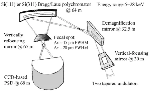
All DiffEXAFS experiments conducted to date have been carried out on ID24, the D-XAS beamline of the ESRF [27] [55], which is shown schematically in figure 3.2.
This result, shown in figure 3.3, means that the equivalent energy of diffracted photons changes continuously along the length of the polychromator, and holds regardless of whether the polychromator is used in Bragg or Laue diffr acting geometries.
The curvature of the crystal also causes each component of the diffracted beam to be focused to a point, at which the sample is placed. Beyond the focal point, the beam diverges and the intensity of each component measured with a position sensitive detector (PSD) - commonly a CCD array. Each pixel in the array only detects a small range of x-ray wavelengths, and so the array as a whole effectively makesnsimultaneous measurements at different x-ray energies, wheren is the number of pixels.
ID24 uses two types of polychromator, both made from a single crystal of silicon. The first is cut and polished with Si(111) or Si(311) planes parallel to the surface and is used for Bragg diffraction at low energies - up to 15 keV. This limit is imposed since higher energy photons penetrate deeply into the crystal, causing significant degradation in energy resolution. The crystal is elliptically bent by a four point bender, with spherical aberrations in the focal spot minimised by cutting the crystal into a specially designed profile that naturally deforms elliptically when bent at its ends. The second type of crystal is cut and polished with Si(111) planes perpendicular to the surface, and is used for Laue diffraction beyond 12 keV and up to about 28 keV. This crystal is bent so as to have a cylindrical profile.
In both cases, the degree of bending is controlled dynamically. This allows both the range of diffracted x-ray wavelengths and the distance to the focused image to be altered. The focal point may lie between 0.8 and 2.0 m from the crystal.
Commonly, D-XAS beamlines are mounted on bending magnet sources, which naturally offer the large spatial divergence (in the horizontal plane) required to generate a wave-length dispersive beam. ID24 however, is unique in that it is mounted on an undulator source.
Figure 3.2: A schematic representation of the optical components of ID24. Reproduced from [55] with modifications.
Figure 3.4: A schematic representation of an undulator/wiggler insertion device. Elec-trons perform small amplitude oscillations, causing the emission of radiation along the axial direction.
oscillations can be approximated by a sinusoid, the device may be characterised by the dimensionless field strength parameter [5]
K= eB0λu
2πmc = 0.934B0(T)λu(cm) (3.7) which in turn gives the maximum angular deviation of the electron [38]
δ= K
γ (3.8)
where λu is the undulator spatial period, B0 is the peak undulator magnetic field
strength, and e, m, and c are the electron charge and mass, and the speed of light respectively.
K is much greater than one for a wiggler, and of the order of one or less for an undulator. This difference has a significant effect on the radiation output from the device. As shown in equation (3.5), the characteristic opening angle of radiation produced by an electron travelling in a circular arc, is of the order of γ−1. Therefore, from (3.8) it can be seen
that in an undulator, the cone of radiation from each electron oscillation is at least partially superimposed upon the radiation cones from previous oscillations, causing x-rays of wavelengthλ1 and its harmonics, to add coherently from one oscillation to the
ID24 Undulator Properties
K value at minimum gap (20 mm) 1.66
Magnet period 42 mm
Number of periods 42
Max. critical energy 8.9 keV
Min. energy of the fundamental 4.4 keV
Max. magnetic field 0.423 T
Source size (x×z RMS) 402 ×8.4µm2
Source divergence (x′×z′ RMS) 12.0×6.2 µrad 2
Peak brilliance at min. gap and 4.5 keV 2.6×10¹⁹ ph s−1mrad−2mm−20.1% BW−10.2˚A−1
Total power emitted 1.34 kW
Power density at 30 m 50.3 Wmm−2 (in central cone at 0.2 ˚A)
Table 3.1: Information pertaining to the undulator source mounted on ID24. These data have been compiled from references [27] and [55].
the squared sum of amplitudes of radiated waves rather than just the sum of radiated wave intensities. Likewise, the oscillatory nature of a wiggler produces a beam as much as several orders of magnitude brighter than a bending magnet source. λ1 is defined by
the undulator period and the electron speed,βe =v/c, as [5]
λ1(θ) =λu
S βe
−cosθ !
(3.9)
Given S, the electron path length over one undulator period, is S= 1 +γ−2K2/4
λ1(θ) =
λu 2γ2 1 +
K2
2 + (γθ)
2
!
(3.10)
whereθ is the angle between the undulator axis and the direction of observation. This equation implies that an undulator source is quasi-monochromatic, with λ1
bandwidth of the undulator to the acceptance of the polychromator, which results in a reduction of specific heat load on the optics.
These all make the beamline ideal for time-resolved analyses of transient chemical reac-tions, and for examination of tiny samples mounted inside high-pressure cells, where the beam must be both highly focused and capable of penetrating the small cell windows. For DiffEXAFS however, these beam characteristics are advantageous for different rea-sons. The lower vertical divergence and resulting smaller focal spot size is ideal since it allows the use of smaller samples, which respond more quickly to small changes in envi-ronmental parameters such as temperature. The reduced specific heat load on the optics is good since it increases the stability of beamline components, minimising unwanted drifts between difference measurements. And most importantly of all, the increased flux is critical in obtaining sufficiently low statistical noise in a DiffEXAFS spectrum to allow signals from phenomena such as thermal expansion or magnetostriction to be detected. These advantages come at a price though. The horizontal divergence of bending magnet sources are typically of the order of several milliradians. Undulator sources however, by their very nature, produce tightly collimated beams, and as such the horizontal divergence of the ID24 source is only12µrad RMS. This requires more complex coupling optics to be installed between the undulator and polychromator in order to generate the required, divergent beam.
ID24 employs two mirrors of Kirkpatrick-Baez (KB) type. The first, mounted 30m from the source, focuses the beam vertically and performs harmonic rejection. The second, orientated at 90◦ with respect to the first at 32.5m from the source, is elliptically bent
to focus the beam horizontally. The focal point, 1.65m from the mirror, then serves as the effective source for the spectrometer, with a horizontal divergence of 1mrad. Consequently, the polychromator, which is mounted 64m from the source, is illuminated over a length of about 40mm. Additional information on the mirrors is given in tables 3.2 and 3.3.