A novel black bone MRI protocol for optimisation of 3D head and neck resection planning

ABSTRACT

Objectives: In current head and neck oncology practice, three-dimensional (3D) virtual planning of resection and reconstruction followed by guided surgery are standard of care. Multimodality imaging fusion introduces a certain inaccuracy in the virtual planning. The aim of this study was to improve the current workflow by developing a method to obtain 3D MRI-based mandible models to avoid multimodality image fusion.

Materials and methods: The study was divided into four phases: a broad exploration phase (1) to define essential MRI related parameters for bone segmentation, a test series (2) with 3 volunteers to optimise the black bone MRI protocol, a validation series with patient data (3) (n=10) for validation of three black bone MRI sequences, and MRI-based guided surgery (4) (n=2) to examine the clinical value. 3D MRI-based models were scored using anatomic ROIs. Surface deviation analysis was performed between CT- and MRI-based models of the validation series. Post-operative evaluation was performed between MRI-based planning and post-operative CBCT data.

Results: The mean deviation values between the reduced MRI-based models and the CT-based models are 0.56, 0.50 and 0.58 mm for the three evaluated black bone MRI sequences. Surgery was performed in two cases with a mean deviation of the saw planes of 2.3 mm, a mean distance between the fibula segments of 3.8 mm, and a mean angle between the axis of the fibula segments of 1.9°

TABLE OF CONTENTS

1 Introduction ... 4

1.1 Goal of the study ... 4

1.2 Study and thesis outline ... 5

2 Background ... 6

2.1 General MRI ... 6

2.2 MRI Parameters ... 8

2.3 MRI Sequences ... 10

2.4 UMCG workflow ... 13

3 Materials and methods ... 14

3.1 Broad exploration phase ... 14

3.2 Test series ... 15

3.3 Validation series ... 16

3.4 MRI-based guided surgery ... 17

4 Results ... 18

4.1 Broad exploration phase ... 18

4.2 Test series ... 18

4.3 Validation series ... 21

4.4 MRI-based guided surgery ... 24

5 Discussion ... 26

6 Conclusion ... 29

1

INTRODUCTION

Patients suffering from malignant or benign oral tumour involving the mandible (lower jaw) or maxilla (upper jaw), are often treated with respectively a partial mandible or maxilla resection followed by a reconstruction of the bone defect using autologous tissue transfer. Often, bone is harvested from e.g. the lower leg (fibula) and transplanted in the mandibular/maxilla defect. This so called fibula free flap reconstruction is a standard procedure in reconstruction of bone defects of the jaws. In current head and neck oncology practice, three-dimensional (3D) virtual planning of resection and reconstruction followed by guided surgery are standard of care [1,2]. Integration of tumour margins to the surgery plan is the factor of success for this workflow. 3D bone models are currently derived from CT data. However, MRI data shows better identification of tumour margins than CT [3]. For a reliable 3D planning, both CT and MRI are used in the diagnostic work up and surgical planning [1]. The workflow requires magnetic resonance imaging (MRI) and computed tomography (CT) or cone beam computed tomography (CBCT) data fusion, to include tumour margins into the pre-surgical plan.

The multimodality data fusion results in an accuracy of 1-2 mm in the surgical plan [4–11]. Eventually, this introduces additional inaccuracies in resection margin planning, which could lead to incomplete removal of tumorous tissue or too small resection margins. Furthermore, mandible resections that are executed with surgical guides also show a deviation of on average 2 mm from the original plan [2]. A planning workflow based on a single modality would make the data fusion step superfluous and excludes the corresponding accuracy error from the surgical plan. MRI is most promising for a single-image-modality planning workflow, since both tumour and bone information can be retrieved from MRI data. Several studies report accurate 3D bone models derived from MRI data [12–24].

1.1

G

OAL OF THE STUDY

The aim of this study is to improve the current workflow for mandible resection and reconstructive surgery planning by developing a method to obtain 3D MRI-based mandible models. The study consists of the introduction of a validated MRI protocol to the clinical workflow, thereby focussing on MRI sequences and settings and segmentation methods. Eventually, this leads to exclusion of the multimodality fusion step from the current planning workflow, thereby improving the accuracy of margin planning.

The research question of this study is:

1.2

S

TUDY AND THESIS OUTLINE

The study is divided into four phases: a broad exploration phase (1) to define essential MRI related parameters for bone segmentation, a test series (2) to optimise the MRI protocol, a validation series (3) for validation of the MRI sequence and segmentation method, and MRI-based guided surgery (4) to examine the clinical value.

2

BACKGROUND

2.1

G

ENERAL

MRI

Magnetic resonance imaging is an imaging technique that uses spins of hydrogen atoms (protons) in the human body to visualise anatomy and pathologies. The working mechanism is based on magnetisation, so the patient is not exposed to ionising radiation. The MRI-scanner consist of a large magnet that creates a magnetic field (B0) that let the magnetic moment of the protons point in two opposite directions, parallel and anti-parallel. The rate of precession of the magnetic moment of the proton is called the Larmor frequency and is related to the field strength of the main magnetic field. The net magnetisation (difference between parallel and anti-parallel aligned protons) is utilised in the formation of an image. Radiofrequency (RF) excitation pulses are send and responding signals are received from protons that spin with the same resonance frequency as the excitation pulse. These excitation pulses are send by a transmitter coil. A receiver coil detects the responding signals. To localise the signals from the body, so called gradients are used. Gradients are short-term spatial variations in magnetic field strength across the patient. These gradients are produced by gradient coils, who are actuated by a controlled pulse sequence.

After an excitation RF pulse, the net magnetisation returns to its equilibrium state by a process called relaxation. Two types of relaxation can be distinguished:

1. The relaxation of the longitudinal magnetisation Mz (direction of the main magnetic field), with the characteristic relaxation time T1.

2. The relaxation of the transverse magnetisation Mxy (direction perpendicular to the main magnetic field), with the characteristic relaxation time T2.

The relaxation of the longitudinal magnetisation can be imagined as rotation back to the z-axis (parallel to B0). Once the RF-pulse stops, the net magnetisation vector in z-direction grows exponentially back to the original situation releasing radiofrequency waves. The longitudinal relaxation time T1 is defined as the time required after a 90° RF-pulse, for growing back to 63% of the initial equilibrium value of M0. T1 relaxation times depend on the type of tissue where the hydrogen nucleus is bound to.

Generally, two types of pulse sequences can be distinguished: spin echo (SE) and gradient echo (GE). To produce an echo that can measure signal intensity, SE sequences use a slice selective 90° excitation RF pulse followed by a 180° rephasing pulse and GE sequences use a single RF pulse followed by a gradient pulse. Both types of sequences make use of echo time (TE) and repetition time (TR). TE is the time between the RF excitation pulse and the echo. TR is the time between the RF excitation pulses. [25,26]

The acquired raw data is temporarily saved in the raw data space: k-space. K-space is a matrix that is filled over time during acquisition. When k-space is sufficiently full, the data is reconstructed by Fourier Transformation to an image. K-space contains a frequency- and phase encoding direction and the size of the matrix corresponds with the size of the final image. Data in the middle of k-space contain low frequency signals (contributing to signal-to-noise and contrast in the image), while high frequency data (contributing to spatial resolution and noise) is stored around the middle [26].

3D MRI

2.2

MRI

P

ARAMETERS

Besides TE and TR, other settings determine signal strength and thereby the quality and contrast of the image. Settings relevant for this study are the flip angle, out of phase imaging, quick FATSAT and GRAPPA.

Flip angle

The flip angle is one of the numerous settings that can be altered in gradient echo sequences. In a standard sequence, the flip angle is set to 90°. In that case, all longitudinal magnetisation flips in the xy-plane at excitation. By shorten the RF pulse, the flip angle will be smaller. A smaller flip angle (α < 90°) results in a small reduction of longitudinal magnetisation and a relatively large reduction of transverse magnetisation (see Figure 1). The total magnetisation signal is still relatively large.

Figure 1 Visualisation of a small flip angle, resulting in a small reduction of longitudinal magnetisation and a relatively

large reduction of transverse magnetisation.

For a proper signal-to-noise-ratio, TR must have a value near the T1 relaxation time. At that moment, the magnetisation is for 63% recovered. To achieve images with an acceptable signal-to-noise-ratio and shorter TR, an RF pulse with a smaller flip-angle is used.

A small flip angle (α ≤ 10°), will result in a more homogeneous image with less contrast between soft tissues [31].

Opposed phase imaging

The opposing phase images are clinically used to identify and quantify the fat content in, for example, liver tissue. Another use of opposed phase imaging is to differentiate adenomas (containing fat) from carcinomas and metastases (not containing fat). [32–34]

Quick FATSAT

One of the solutions to overcome disturbing bright fat signal is to use fat saturation. As known, fat and water protons have a slightly different resonance frequency. Therefore, the protons bound to fat can be excited by a narrow band specific RF pulse. Immediately after the excitation of the fat protons, a spoiler gradient destroys the fat signal. This process is called ‘saturation’. The result is an image where the water bound protons are visualised as bright, and the fat bound protons are black. The fat-selective excitation pulse is given before each normal excitation pulse. For good selectivity, the FATSAT pulse must have a certain duration. This makes the acquisition time of the sequence significantly longer. The MAGNETOM quick FATSAT pulse (Siemens) results in shorter acquisition times by applying the FATSAT pulse less frequently, while maintaining the image quality. [35,36]

GRAPPA

2.3

MRI

S

EQUENCES

A broad exploration of appropriate MRI sequences for bone segmentation is performed in this study. The characteristics and common applications of these sequences are outlined in this section.

2.3.1

VIBE

Goto et al. [21] have investigated the accuracy of several (3D) MRI sequences for measurements of the mandible. The optimal MRI sequence was determined to be 3D volumetric interpolated breath-hold examination (VIBE).

The so called VIBE sequence is an ultrafast gradient echo (GE) sequence available in Siemens MRI scanners. The sequence is designed as a result of disappointing image quality in 3D gradient echo imaging because of relatively limited resolution and anatomic coverage in abdomen imaging [39]. The sequence is optimized for short acquisition times and the resolution is improved by asymmetric filling of k-space. VIBE is frequently used in abdominal imaging [30], however, the sequence is also applied in brain imaging [40].

2.3.1.1

D

VIBE

A variation of the standard VIBE sequence, Dixon VIBE, is also explored in this study. The Dixon sequence relies on difference in resonance frequency between water and fat molecules. This difference is used to create in-phase and out of phase images (see opposed phase imaging in section 2.2). When fat and water protons are in-phase, the signal of the voxel is the sum of the two signal vectors of both fat and water. So the image shows the strongest signal at fat and water rich areas. Inversely, when the fat and water protons are in opposed phase, the signal of the voxel is the difference between water and fat vectors. The resulting image is a fat-suppressed image. By adding and subtracting these in- and out of phase images, fat- and water-only images are created. Thus, the results of a Dixon sequence are four separate and different data sets. [41–43].

The combination of VIBE and Dixon results in a fast and high resolution 3D MRI sequence that produces four images: in-phase, out of phase, fat-only and water-only images. The four different images could each contribute to the segmentation of bone, since different contrasts between the tissues are obtained. The Dixon technique is utilised in in combination with a 3D dual echo-time sequence in a study of Gyftopoulos et al. [44] for 3D bone reconstructions of the shoulder.

2.3.1.2

VIBE

phase encoding direction. By changing the k-space filling pattern, sensitivity to motion and patient movement is reduced. In a radial sampling scheme, the data is acquired along rotated ‘spokes’. The overlap of the spokes in the center predominates the potential jittering of the spokes. Therefore, gaps in k-space coverage will not occur. The overlap of the spokes also averages the motion in an image. A downside of this radial sampling method is the appearance of streak artifacts. Imaging of the head and neck region benefits from the starVIBE sequence, since involuntary movements (swallowing, eye blinking, breathing) disturb the image quality in that region. [45–47]

2.3.2

MPRAGE

Iacono et al. [23] utilised, among others, a 3D magnetisation prepared rapid acquisition gradient-echo sequence (MPRAGE) sequence for a detailed anatomic model of the human head and neck. This sequence consists of a magnetisation preparation (MP), followed by a rapid gradient echo (RAGE) sequence to sample the prepared magnetisation [48]. It is also called a “IR-prepped” sequence [49]. The sequence consists of three steps: magnetisation preparation, acquisition, and magnetisation recovery. The preparatory module contains a 180° inversion pulse. For MPRAGE, the acquisition consists of rapid gradient echo. The magnetisation recovery allows the system to return to its equilibrium. The MRPAGE sequence is a frequently utilised sequence in imaging the brain, because of excellent tissue contrast, high spatial resolution, and full brain coverage in a short scan time [50].

2.3.3

TSE

Iacono et al. [23] also utilised a 3D turbo spin echo (TSE) sequence for the detailed anatomic model of the human head and neck. The TSE sequence is a commonly used sequence in diagnostic imaging. It uses a series of 180° pulses and echo’s after the 90 – 180° pulses of conventional spin echo sequences. The phase encoding gradient changes in this technique, and multiple lines of k-space can be acquired in the same repetition interval (TR). This reduces the acquisition time. Besides time saving, TSE also has the advantage that susceptibility-induced signal losses are reduced. [25,51]

2.3.4

FLAIR

Fluid-attenuated inversion recovery (FLAIR) sequences are not mentioned in literature for bone segmentation, however, it is commonly utilised in diagnostic imaging and datasets were available to explore usefulness for bone segmentation and 3D modelling. A long inversion time results in suppression of liquor [25]. FLAIR sequences are utilised in brain imaging when lesions are close to the ventricles [26].

2.3.5

B

parallel lines, that are acquired with a fixed angle relative to each other [25]. If the blade consisted of only one line of raw data, it would be equal to radial acquisition. The advantage of PROPELLER (or blade) is the reduction of motion artefacts due to oversampling the centre of k-space [26].

2.3.6

B

2.4

UMCG

WORKFLOW

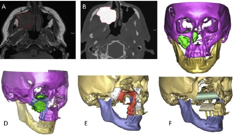
This section describes the currently used three-dimensional (3D) pre-surgical virtual planning workflow for reconstructive surgery of the head and neck region in the UMCG. Figure 2 shows an impression of the workflow from Kraeima et al. [1].

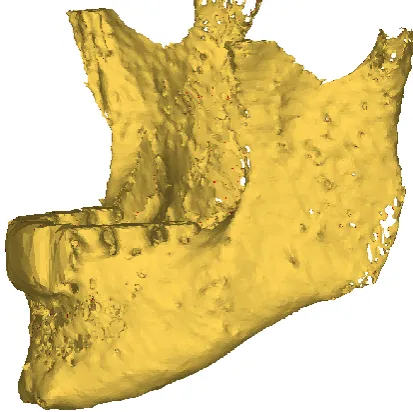
In the planning process, CT images are necessary to visualise and segment bony structures. Additionally, to design the surgery plan, the area of tumour need to be identified. CT images do not (clearly) show this tumour, so MRI data of the head and neck region is used to delineate tumour mass and location (Figure 2A). Eventually, these two image sets are fused, to show the bone/tumour relationship (Figure 2B). This is important to decide where to place the resection margins. To merge the tumour margins from MRI to the CT data, a Matlab-algorithm is used [1] . From the CT data (including tumour margins), important structures are segmented into 3D objects (Figure 2C). Essential structures are the fibula/crista, mandible/maxilla and tumour. Then, the surgery can be virtually planned on the 3D models (Figure 2D). Cutting planes are determined for both the mandible and the fibula/crista. Based on these cutting planes, resection guides are designed to perform the surgery exact as planned (Figure 2E). Finally, the bony reconstruction parts (fibula or crista) are virtually placed (Figure 2F). The plan, the resection guides, and sometimes a patient specific reconstruction plate (designed using the obtained 3D models) are utilised to perform the surgery exactly as planned.

Figure 2 Impression of the currently used UMCG planning workflow (images from Kraeima et al. [1]) A Tumour

3

MATERIALS AND METHODS

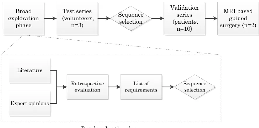
For obtaining 3D MRI-based mandible models, a four phase approach was defined: broad exploration phase to define essential MRI related parameters for bone segmentation (1), test series of the most relevant MRI settings (2), validation series of the selected MRI parameters (3), and MRI-based virtual planning for tumour surgery of oral squamous cell carcinoma (4) (see Figure 3).

Figure 3 Schematic outline of the workflow of this study showing the four phases: broad exploration phase to define

essential MRI related parameters for bone segmentation, test series of the most relevant MRI settings, validation series of the selected MRI parameters, and MRI-based virtual planning for tumour surgery of an oral squamous cell carcinoma. The rhombic boxes show decision making moments in the workflow.

3.1

B

ROAD EXPLORATION PHASE

A literature search was performed for finding the essential MRI parameters for bone segmentation. The search was performed in Web of Science with the following search strategy: “bone segmentation MRI”, “3D bone model MRI”, and “mandible bone segmentation MRI”. The purpose was not to perform a systematic review, because it was considered not necessary for finding MRI settings from the literature. The search yielded 23 papers describing segmentation of bone from MRI (see Table A-1, Appendix A ). The most relevant settings were selected by a radiologist and an MRI scientist.

without Gadolinium contrast medium). These sequences are routinely available on a 3 Tesla MAGNETOM PRISMA (Siemens) MRI-scanner. The quality of the 3D mandible models that could be generated from the retrospective MRI data was evaluated focussing on contrast between mandible and surrounding tissue, (3D) scanning protocol, time of segmentation, quality of 3D models (compared to CT-based 3D models when available). Based on literature study and the quality of the obtained 3D models of the mandible, requirements were defined for MRI sequences, scan resolution and slice thickness as well as segmentation methods suitable for 3D planning. A single MRI sequence was selected for further optimisation and validation.

3.2

T

EST SERIES

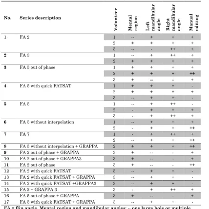
For optimisation of the pre-selected sequence, a test series on three healthy volunteers was performed. The black bone sequence, described by Eley et al. [31], acted as starting point sequence. In the optimisation process, the flip angle was modified, as well as addition of fat saturation (quick FATSAT), scanning without interpolation (standard = with interpolation), addition of GeneRalized Autocalibrating Partial Parallel Acquisition (GRAPPA), and out of phase scanning was performed. The flip angles varied between 2˚ and 7° to see the effect on soft tissue-mandible contrast and reciprocal contrast of soft tissues. Segmentation of the tissue-mandible is only possible when there is clear soft tissue-mandible contrast, while it is desirable to have minimal soft tissue contrast. Application of quick FATSAT results in a nulled signal of fat (black in the images), leading to a more balanced contrast in the image and darker visualization of cancellous bone (less contrast between cortical and cancellous bone). Scanning without interpolation was performed to avoid the rough surface of the 3D models. GRAPPA is a parallel imaging technique, resulting in shorter scanning times. It can halve or double halve (GRAPPA3) the acquisition time. The shorter acquisition is especially beneficial in head and neck imaging, due to frequent occurring movement artefacts. Finally, out of phase scanning was performed, since this results in small black lines on tissue borders. These black line artefacts might be useful for segmentation of the bones. More information about these parameters is outlined in section 2.2.

All series were performed on a 3T MRI-scanner (MAGNETOM Prisma, Siemens, Erlangen, Germany) using a 64-channel head coil and a region of interest (ROI) containing at least the complete mandible. Extra fixation of the head was accomplished with foam pillows or towels. The volunteers were positioned supine and head first, as in the conventional protocol. The standard series was a black bone VIBE sequence with interpolation. Slice thickness and pixel size were set on 0.7 mm for all series.

following smoothing setting were applied: smoothing factor 0.8, iterations 5, compensate shrinking on (see Appendix C ).

Scoping of the sequences towards selection of the optimal black bone sequence was based on the quality of the 3D models. Each segmentation was scored by one observer. Anatomical ROIs for cutting guide designs were defined based on a retrospective evaluation of seventeen mandible cutting guide designs that were previously used for oral cancer surgery with removal of a part of the mandible. This led to the definition of three ROIs for quality evaluation. The scoring system of the 3D mandible models included the number of virtual holes in the mental region, the number of holes in the left and right mandibular angles, and the number of manual deleted attachments. The three best scoring sequences were chosen to use in the validation series.

3.3

V

ALIDATION SERIES

In this series, the three selected black bone sequences were validated using patient data. The goal of this validation series was to select the most promising black bone sequence settings for 3D modelling of the mandible via surface comparison of CT- and MRI-based models.

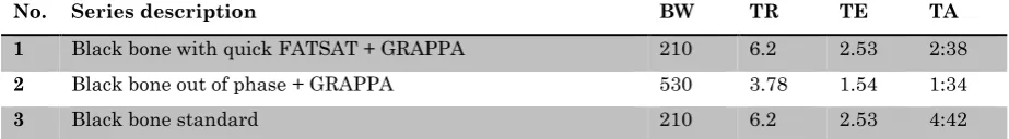
Ten patients with oral cancer undergoing MRI and CT imaging of the tumour as part of the diagnostic work up were prospectively selected. The three black bone sequences were added to the conventional MRI protocol, which increased scanning time with less than 10 minutes. All series were performed on a 3T MRI-scanner (MAGNETOM Prisma, Siemens, Erlangen, Germany) using a 64-channel head coil. The patients were positioned supine and head first. Gadolinium contrast material was administered following regular protocol before the black bone series were performed. Table 1 shows the three black bone sequences with its parameters. The flip angle was 2°. Pixel size and slice thickness were 0.7 mm in all sequences.

Table 1 Sequences and characteristics of validation series. The sequences are all variations on the black bone sequence.

No. Series description BW TR TE TA

1 Black bone with quick FATSAT + GRAPPA 210 6.2 2.53 2:38

2 Black bone out of phase + GRAPPA 530 3.78 1.54 1:34

3 Black bone standard 210 6.2 2.53 4:42

BW = pixel bandwidth (Hz/pixel), TR = Repetition time (ms), TE = Echo time (ms), TA = acquisition time (min)

Scoring was performed according to the method used in the test series, in order to evaluate the quality of the 3D MRI-based models. Next to that, a quantitative surface comparison of the 3D MRI- and CT-based models was made. First, a surface match was performed using an iterative closest point (ICP) algorithm in Geomagic Studio 2012.0.0 (Geomagic GmbH). Then, three planes were created to remove parts of the mandible of both the aligned MRI- and CT-based models using 3-Matic Medical 10.0 (Materialise, Leuven, Belgium) maintaining the anatomical ROIs based on the cutting guide designs (defined in section 3.2). The analysis was completed by a part to part comparison of the reduced models. Mean deviation and distance maps showed the deviation (absolute value) of CT- and MRI-based models.

3.4

MRI-

BASED GUIDED SURGERY

Guided resection and reconstruction surgery, based on MRI, was performed in two cases of patients with oral cancer of which the surgical plan included removal of a part of the mandible. MRI data of both patients were also used in the validation series.

The cases involved T4 squamous cell carcinoma of the oral cavity requiring resection of the mandible followed by (segmented) fibula reconstruction of the defect. The patients diagnostic and tumour surgery workup were not altered from the conventional workflow, including the preoperative 3D virtual planning procedure [1]. MRI data was used for 3D bone modelling and resection planning using ProPlan CMF 1.3 (Materialise, Leuven, Belgium) based on tumour outline obtained from other MRI sequences.

4

RESULTS

4.1

B

ROAD EXPLORATION PHASE

Based on literature search and segmentation of several sequences, a list of requirements is described Table D-2. The 3D black bone VIBE sequence was selected as starting point for further optimisation. A detailed description of the segmentation examples and the list of requirements are elaborated in Appendix D .

4.2

T

EST SERIES

Table 2 shows the quality assessment of the mandible bone segmentations from the three volunteers. Inter-subject differences were found between the 3D models of the same sequences. Differences between the 3D models of the same sequences are noticeable. E.g., the 3D model of the out of phase sequences with a flip angle of 5° shows poor segmentation quality in both mandibular angles in one case, while the segmentation quality in those areas was assessed as sufficient in the 3D models of the other two volunteers. Another notable result is the poor segmentation quality in the mental region in the FA 5 with quick FATSAT model compared to the good segmentation in that area in the models of the other volunteers.

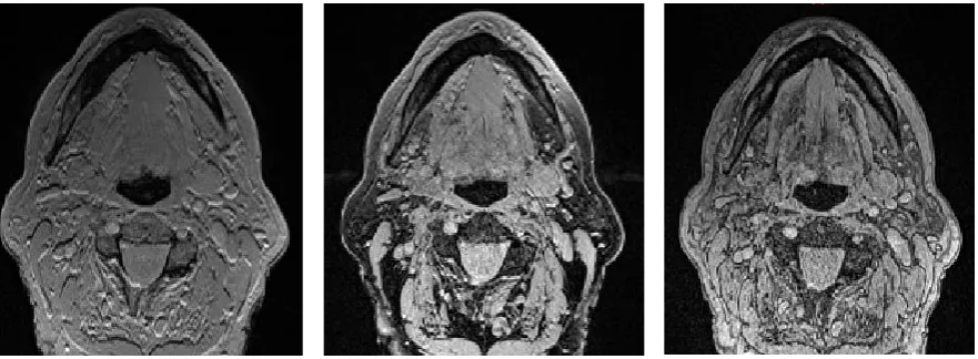
Despite the reported inter-subject inconsistencies, in general equal segmentation quality results can be observed. The sequences without the use of quick FATSAT or out of phase imaging show bad segmentation in the mental region (see Figure 4). The images show interruption of the black boundary in that area. The sequences with quick FATSAT settings generally need more manual editing to remove additional attachments, where the out of phase sequences need less manual editing, but the segmentation quality of the mandible angles is impaired (see Figure 5). The influence of GRAPPA and GRAPPA 3 is not visible in the segmentation quality.

Table 2 Segmentation quality scoring of each 3D mandible model derived from the test series. The starting point is the

black bone MRI sequence.

No. Series description

Vo lu n teer M en ta l regi on Lef t m and ib u lar angl e Rig h t m and ib u lar angl e M anu al edit in g

1 FA 2 1 -- + + +

2 + + + +

3 -- - ++ +

2 FA 3 1 -- + ++ +

2 + + + +

3 FA 5 out of phase 1 + + + +

2 + + + ++

3 + -- - +

4 FA 5 with quick FATSAT 1 + + + -

2 + + + +

3 -- + + -

5 FA 5 1 -- + ++ -

2 - + + +

3 - + ++ +

6 FA 5 without interpolation 1 -- + + +

2 - + + ++

7 FA 7 1 - + ++ +

2 -- + + ++

8 FA 5 without interpolation + GRAPPA 2 + + + ++

9 FA 2 out of phase + GRAPPA 3 + -- - +

10 FA 2 out of phase + GRAPPA3 3 + -- - +

11 FA 2 out of phase 3 + -- - ++

12 FA 2 with quick FATSAT 3 -- + + -

13 FA 2 with quick FATSAT + GRAPPA 3 -- + + -

14 FA 2 with quick FATSAT +GRAPPA3 3 -- + + -

15 FA 2 + GRAPPA 3 3 - + ++ +

16 FA 5 out of phase + GRAPPA 3 + -- - +

17 FA 5 with quick FATSAT + GRAPPA 3 -- + + -

Figure 4 Impaired segmentation quality of the mental region showed in axial and sagittal slices and the 3D model

derived from the standard black bone MRI sequence of the test series with a flip angle of 2˚. The interruption of the black boundary (cortical bone) creating the virtual holes in the model is visible in the slices.

Figure 5 Impaired segmentation quality (virtual holes) visible in the left mandibular angle in the 3D model derived from

The most adequate segmentations were chosen with the knowledge that a smaller flip angle gives a more homogenous aspect with less contrast in soft tissue. Therefore, a flip angle of 2° was chosen. To evaluate the differences between quick FATSAT, out of phase imaging and scanning without quick FATSAT and out of phase in a larger (patients)group, these three sequences were selected to use in the validation series.

4.3

V

ALIDATION SERIES

Most scans required extensive manual editing resulting in a long segmentation process (30-60 minutes per 3D mandible model). In most cases, the standard scan (without quick FATSAT or out of phase scanning) needed less manual editing (see Table 3). The series performed with GRAPPA shows more noise compared to the images obtained without GRAPPA. These series also show more soft tissue contrast (see Figure 6). Movement artefacts were visible in the series of patients 4 and 5. Metal artefact caused by implants were visible in the images of patients 6 and 10.

The average error of the alignment measurements of CT- and MRI-based models indicates the average deviation of all points of comparison. This indicates the accuracy of alignment. The models are aligned within an average accuracy of 0.7 mm.

Table 3 Segmentation quality scoring of each 3D mandible model derived from the validation series

No. Series Mental

region Left mandibular angle Right mandibular angle Manual editing

1 A + - - --

B + + + --

C + ++ ++ -

2 A ++ + ++ -

B ++ - + -

C + + ++ +

3 A + + +

--B + - +

-C -- - -

--4 A - - + --

B ++ + + --

C -- - + --

5 A + + + --

B + + + --

C ++ ++ ++ +

6 A + + + --

B + - - --

C + + + +

7 A ++ + ++ --

B ++ + + --

C - + ++ +

8 A + - - -

B + - - --

C ++ -- - -

9 A ++ ++ ++ -

B ++ + ++ -

C ++ + ++ +

10 A + + + --

B + + + --

C + + + +

A = FA 2 FATSAT with GRAPPA, B = FA 2 out of phase with GRAPPA, C = FA 2. Mental region and mandibular angles: -- one large hole or multiple large holes; - multiple holes; + view holes; ++ no holes. Manual editing: -- more than 15 parts edited; - 10-15 parts edited; + 5-10 parts edited; ++ less than 5 parts edited.

Figure 6 Axial views of (from left to right) standard black bone MRI sequence, black bone with quick FATSAT +

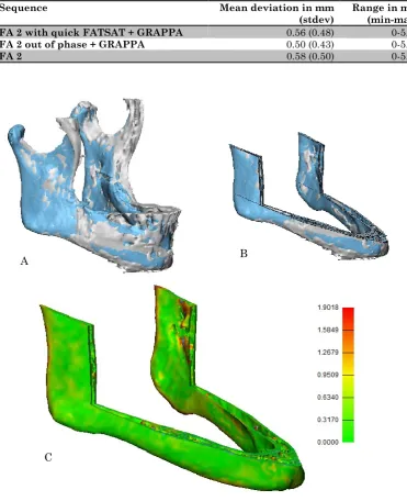
Table 4 Mean values and standard deviation of the deviation analysis measurements between CT- and MRI-based

models. This analysis is performed after reduction of the models by three cutting planes, maintaining the ROI for comparison.

Sequence Mean deviation in mm

(stdev) Range in mm (min-max) FA 2 with quick FATSAT + GRAPPA 0.56 (0.48) 0-5.35

FA 2 out of phase + GRAPPA 0.50 (0.43) 0-5.90

FA 2 0.58 (0.50) 0-5.43

Figure 7 A Aligned CT- (blue) and MRI-based (grey) models. B Reduced aligned CT- (blue) and MRI-based (grey) models,

showing the region of interest for comparison. C Distance map of the reduced models. The CT-based model is analysed and compared to the MRI-based model.

B

4.4

MRI-

BASED GUIDED SURGERY

The most adequate segmented sequence of a patient with a T4 oral tumour, black bone with quick FATSAT + GRAPPA and a flip angle of 2°, was selected to use for PSP design and surgical margin planning. For the second MRI-based guided surgery, the black bone sequence with a flip angle of 2˚ was utilised (see Figure F-1, Appendix F ).

The virtual evaluation of the test plate shows proper fitting of the MRI-based plate (see Figure F-2, Appendix F ). In the mental region, as well as in the region where the masseter muscle overlays the mandible (both right and left side), the test plate shows a small deviation from the model. On the top side of the ramus, both right and left side, the test plate shows a minimal deviation with an anterior opening between plate and bone surface. The virtual fitting of the test plate together with the expert opinion from the surgeon were decisive for planning the surgery on the MRI-based models.

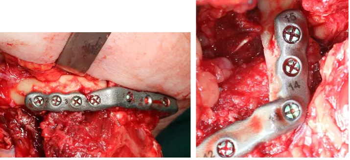
The 3D printed PSP placed on the 3D printed reconstruction model is shown in Figure 8. The virtual surgical reconstruction plans of both cases are shown in Figure 9.

Figure 10 shows the PSP connected to the two fibula segments during surgery. The fibula segments are connected to each other and to the original mandible bone without gaps and there is no deviation between bone and plate visible.

The post-operative evaluation resulted in a mean distance between the midpoints of the saw planes of 2.3 mm. The mean distance between the centre points of the fibula segments was 3.8 mm and the mean angle between the axis of the fibula segments was 1.9°.

Figure 8 3D printed patient specific reconstruction plate (PSP) placed on the 3D printed mandible reconstruction model

Figure 9 Virtual surgical plan of first case (left) and second case (right) showing the 3D MRI-based mandible models

(white), fibula segments (green and blue), patient specific reconstruction plate (grey, left case) and the cutting guides (yellow, right case).

Figure 10 MRI-based patient specific reconstruction plate (PSP) connected to the fibula parts during surgery showing a

5

DISCUSSION

This study reports an optimisation of the 3D virtual planning workflow, by providing an MRI (bone) protocol for 3D mandible segmentation and resection planning. The use of this protocol would make multimodality image fusion superfluous in virtual planning for guided surgery.

The validation method, surface comparison with the gold standard 3D CT-based models, showed average deviation errors between 0.5 and 0.6 mm. In this analysis, the coronoid process and the mandibular condyles of the mandible models were discarded, because these areas were difficult to separate from muscle attachment (coronoid process) and are not relevant in reconstructive planning. Even though this reflects limitation of segmenting 3D mandible models from MRI data, it was possible to plan surgical resection guides and a reconstruction plate from the MRI data in two patients.

MRI is sensitive for artefacts, mainly caused by metal and patient movement. The influence of metal was visible in the test series of one of the volunteers (see Figure E-1, Appendix E ), and in two patients of the validation series. Especially the scans with FATSAT show large artefacts. This is, however, not influencing the segmentation quality of the mandible, since it is restricted to the level of the dentition. In comparison with CT, that shows scattering artefacts from dental fillings, these metal artefacts will not lead to problems in daily patient care. Two series of the validation series shows impaired image quality caused by movement artefacts. It was anticipated that scanning quality would be influenced by movement artefacts, since it is difficult for patients to lie still in the MRI-scanner for more than half an hour. Moreover, swallowing and breathing also causes movement artefacts. Fortunately, almost all patients were able to lie still and the swallowing and breathing motion did not disturb the segmentation quality. The short acquisition times (max. 4 minutes) also contributed to the absence of artefacts.

The test series did not show any differences in segmentation quality between images obtained with GRAPPA, GRAPPA3 or without GRAPPA. However, the data of the validation series obtained with GRAPPA, needed more manual editing compared to the data scanned without the use of GRAPPA. More noise was observed in the GRAPPA images, one of the disadvantages of the faster scanning method and a possible explanation of bad segmentation quality. The impaired segmentation quality could also be explained by the fact that out of phase imaging and addition of FATSAT cancel out the effect of low soft tissue contrast caused by the low flip angle, as seen in Figure 6.

Marginal differences between results of the validation series resulted in a hard selection process for the best sequence for segmentation and 3D modelling of the mandible needed for 3D margin and reconstruction planning. The three sequences of the validation series all meet the

scanning. However, for the first clinical case, the sequence scanned with quick FATSAT and GRAPPA, proved to be a proper and accurate sequence for this purpose as well. Since

segmentation time is really important for application in clinical routine, the standard black bone sequence is preferred. It is advised to add the other sequences to the scanning protocol as well if time and situation permits.

Strengths and weaknesses

Despite the exclusion of the multimodality component in this workflow, data fusion is still required. Diagnostic MRI sequences are combined with the black bone MRI sequence for optimal tumour and bone information in the virtual planning. However, this ‘fusion’ between MRI data from the same series is more accurate, since it is obtained in the same patient positioning and the same moment of time.

Acquiring 3D mandible models from CT data is relatively simple and does not require long segmentation times. Creating 3D mandible models based on MRI data, however, take some time, due to the required manual editing. The additional segmentation time is estimated at 30 minutes per 3D mandible model for MRI-based segmentation. On the other hand, segmenting from MRI saves time in the planning workflow, since no fusion of different image modalities is needed.

Relate to current literature

As far as known, this paper describes the first case where black bone MRI is utilized in 3D virtual resection margin planning. Eley et al. have described the role of black bone MRI for radiation reduction in craniofacial imaging [31], for cephalometric analysis [52], and as potential alternative to CT in 3D reconstruction of the craniofacial skeleton [53]. Radetzki et al. [54] used a black bone MRA sequence for virtual simulation and evaluation of the femoralacetabular impingement. Robinson et al. [55] have described the utility of black bone MRI in assessment of the foetal spine. So, bone segmentation from MRI is described before, however, using MRI for 3D virtual resection margin planning in head and neck oncologic reconstruction surgeries is not reported before and thus a novel and inventive protocol is outlined.

Recommendations for future research

This study describes two successful cases where a patient specific reconstruction plate and mandible surgical guides were designed based on 3D MRI models. A prospective clinical trial must be performed to support the added value for the current 3D planning workflow in terms of improved resection margin planning, since evaluation of free bone margins is not included in this study.

bone MRI, so segmentation difficulties are expected due to air in the sinuses connected to the maxilla.

Implications for current practice

Using MRI data instead of CT data for production of 3D bone models of the mandible will eventually lead to more accurate margin planning, by avoiding the CT-MRI fusion step. A more accurate and reliable margin planning might possibly lead to smaller resection margins. The omission of data fusion will also lead to an optimised workflow. Since the planning workflow already consists of several steps, a shorter workflow is desirable and will contribute to better patient treatment.

6

CONCLUSION

The aim of this study was to improve the current workflow for mandible resection and reconstructive surgery planning by developing a method to obtain 3D MRI-based mandible models. The corresponding research question was:

“Can a clinical effective method be developed for generation of three-dimensional models of the mandible, suitable for three-dimensional pre-surgical margin planning and based on magnetic resonance imaging?”

7

REFERENCES

[1] Kraeima J, Schepers RH, van Ooijen PMA, Steenbakkers RJHM, Roodenburg JLN, Witjes MJH. Integration of oncologic margins in three-dimensional virtual planning for head and neck surgery, including a validation of the software pathway. J Cranio-Maxillofacial Surg 2015;43:1374–9. doi:10.1016/j.jcms.2015.07.015.

[2] Schepers RH, Raghoebar GM, Vissink A, Stenekes MW, Kraeima J, Roodenburg JL, et al. Accuracy of fibula reconstruction using patient-specific CAD/CAM reconstruction plates and dental implants: A new modality for functional reconstruction of mandibular defects. J Craniomaxillofac Surg 2015;43:649–57. doi:10.1016/j.jcms.2015.03.015.

[3] Brown JS, Griffith JF, Phelps PD, Browne RM. A comparison of different imaging modalities and direct inspection after periosteal stripping in predicting the invasion of the mandible by oral squamous cell carcinoma. Br J Oral Maxillofac Surg 1994;32:347–59. doi:10.1016/0266-4356(94)90024-8.

[4] van Herk M, Kooy HM. Automatic three-dimensional correlation of CT-CT, CT-MRI, and CT-SPECT using chamfer matching. Med Phys 1994;21:1163–78. doi:10.1118/1.597344.

[5] Khoo VS, Dearnaley DP, Finnigan DJ, Padhani A, Tanner SF, Leach MO, et al. Magnetic resonance imaging (MRI): considerations and applications in radiotherapy treatment planning. Radiother Oncol 1997;42:1–15. doi:http://dx.doi.org/10.1016/S0167-8140(96)01866-X.

[6] Mongioj V, Brusa A, Loi G, Pignoli E, Gramaglia A, Scorsetti M, et al. Accuracy evaluation of fusion of CT, MR, and spect images using commercially available software packages (SRS PLATO and IFS). Int J Radiat Oncol Biol Phys 1999;43:227–34. doi:10.1016/S0360-3016(98)00363-0.

[7] Mutic S, Dempsey JF, Bosch WR, Low D a, Drzymala RE, Chao KS, et al. Multimodality image registration quality assurance for conformal three- dimensional treatment planning. Int J Radiat Oncol Biol Phys 2001;51:255–60.

[8] Krempien RC, Daeuber S, Hensley FW, Wannenmacher M, Harms W. Image fusion of CT and MRI data enables improved target volume definition in 3D-brachytherapy treatment planning. Brachytherapy 2003;2:164–71. doi:10.1016/S1538-4721(03)00133-8.

[9] Wang X, Li L, Hu C, Qiu J, Xu Z, Feng Y. A comparative study of three CT and MRI registration algorithms in nasopharyngeal carcinoma. J Appl Clin Med Phys 2009;10:3–10. doi:10.1120/jacmp.v10i2.2906.

CT/MR image registration. Int J Radiat Oncol Biol Phys 2010;77:1584–9. doi:10.1016/j.ijrobp.2009.10.017.

[11] Dean CJ, Sykes JR, Cooper RA, Hatfield P, Carey B, Swift S, et al. An evaluation of four CT-MRI co-registration techniques for radiotherapy treatment planning of prone rectal cancer patients. Br J Radiol 2012;85:61–8. doi:10.1259/bjr/11855927.

[12] Van den Broeck J, Vereecke E, Wirix-Speetjens R, Vander Sloten J. Segmentation

accuracy of long bones. Med Eng Phys 2014;36:949–53.

doi:10.1016/j.medengphy.2014.03.016.

[13] Rathnayaka K, Momot KI, Noser H, Volp A, Schuetz M a., Sahama T, et al. Quantification of the accuracy of MRI generated 3D models of long bones compared to CT generated 3D models. Med Eng Phys 2012;34:357–63. doi:10.1016/j.medengphy.2011.07.027.

[14] Biedert R, Sigg A, Gal I, Gerber H. 3D representation of the surface topography of normal and dysplastic trochlea using MRI. Knee 2011;18:340–6. doi:10.1016/j.knee.2010.07.006.

[15] Ababneh SY, Prescott JW, Gurcan MN. Automatic graph-cut based segmentation of bones from knee magnetic resonance images for osteoarthritis research. Med Image Anal 2011;15:438–48. doi:10.1016/j.media.2011.01.007.

[16] Fripp J, Bourgeat P, Crozier S, Ourselin S. Segmentation of the Bones in MRIs of the Knee Using Phase, Magnitude, and Shape Information. Acad Radiol 2007;14:1201–8. doi:10.1016/j.acra.2007.06.021.

[17] Dodin P, Martel-Pelletier J, Pelletier J-P, Abram F. A fully automated human knee 3D MRI bone segmentation using the ray casting technique. Med Biol Eng Comput 2011;49:1413–24. doi:10.1007/s11517-011-0838-8.

[18] Kraiger M, Martirosian P, Opriessnig P, Eibofner F, Rempp H, Hofer M, et al. A fully automated trabecular bone structural analysis tool based on T2*-weighted magnetic resonance imaging. Comput Med Imaging Graph 2012;36:85–94. doi:10.1016/j.compmedimag.2011.07.006.

[19] Arezoomand S, Lee WS, Rakhra KS, Beaulé PE. A 3D active model framework for segmentation of proximal femur in MR images. Int J Comput Assist Radiol Surg 2014:55– 66. doi:10.1007/s11548-014-1125-6.

[20] Włodarczyk J, Czaplicka K, Tabor Z, Wojciechowski W, Urbanik A. Segmentation of bones in magnetic resonance images of the wrist. Int J Comput Assist Radiol Surg 2015;10:419– 31. doi:10.1007/s11548-014-1105-x.

accuracy of 3-dimensional magnetic resonance 3D vibe images of the mandible: an in vitro comparison of magnetic resonance imaging and computed tomography. Oral Surgery, Oral Med Oral Pathol Oral Radiol Endodontology 2007;103:550–9. doi:10.1016/j.tripleo.2006.03.011.

[22] Ji DX, Foong KWC, Ong SH. A two-stage rule-constrained seedless region growing approach for mandibular body segmentation in MRI. Int J Comput Assist Radiol Surg 2013;8:723–32. doi:10.1007/s11548-012-0806-2.

[23] Iacono MI, Neufeld E, Akinnagbe E, Bower K, Wolf J, Vogiatzis Oikonomidis I, et al. MIDA: A Multimodal Imaging-Based Detailed Anatomical Model of the Human Head and Neck. PLoS One 2015;10:1–35. doi:10.1371/journal.pone.0124126.

[24] Eley KA, Watt-Smith SR, Golding SJ. “Black bone” MRI: a potential alternative to CT when imaging the head and neck: report of eight clinical cases and review of the Oxford experience. Br J Radiol 2012;85:1457–64. doi:10.1259/bjr/16830245.

[25] Brix G, Kolem H, Nitz WR. Basics of Magnetic Resonance Imaging and Magnetic Resonance Spectroscopy. Magn. Reson. Tomogr., 2008.

[26] McRobbie D et al. MRI: From Picture to Proton. vol. 85. 2003. doi:10.1097/00004032-200310000-00020.

[27] Hoa D. IMAIOS 3D spatial encoding n.d. https://www.imaios.com/en/e-Courses/e-MRI/Signal-spatial-encoding/3D-spatial-encoding.

[28] Hornak JP. The Basics of MRI - basic imaging techniques n.d. https://www.cis.rit.edu/htbooks/mri/chap-8/chap-8.htm.

[29] Naraghi A, White LM. Three-Dimensional MRI of the Musculoskeletal System. Am J Roentgenol 2012;199:W283–93. doi:10.2214/AJR.12.9099.

[30] Papanikolaou N, Karampekios S. 3D MRI Acquisition: Technique. Image Process Radiol 2008:15–26.

[31] Eley KA, Mcintyre AG, Watt-Smith SR, Golding SJ. “Black bone” MRI: a partial flip angle technique for radiation reduction in craniofacial imaging. Br J Radiol 2012;85:272–8. doi:10.1259/bjr/95110289.

[32] Elster AD. Chemical Shift: 2nd kind 2015. http://mri-q.com/chemical-shift-2nd-kind.html.

[33] Elster AD. In-phase v Out-of-phase 2015. http://mri-q.com/in-phaseout-of-phase.html.

imaging: a useful tool for evaluating more than fatty infiltration or fatty sparing. Radiographics 2006;26:1409–18. doi:10.1148/rg.265055711.

[35] Purdy D. MRI Hot topics - The Skinny on FATSAT 2009.

[36] Elster AD. CHESS/Fat-Sat Pulses 2015. http://mri-q.com/fat-sat-pulses.html.

[37] Zähringer C, D THM, Sommer G, Bongartz G. MAGNETOM Prisma – Abdominal Applications 2014:6–11.

[38] Elster AD. GRAPPA/ARC 2015. http://mri-q.com/grappaarc.html.

[39] Rofsky NM, Lee VS, Laub G, Pollack M a, Krinsky G a, Thomasson D, et al. Abdominal MR imaging with a volumetric interpolated breath-hold examination. Radiology 1999;212:876–84. doi:10.1148/radiology.212.3.r99se34876.

[40] Viallon M, Cuvinciuc V, Delattre B, Merlini L, Barnaure-Nachbar I, Toso-Patel S, et al. State-of-the-art MRI techniques in neuroradiology: principles, pitfalls, and clinical applications. Neuroradiology 2015;57:441–67. doi:10.1007/s00234-015-1500-1.

[41] Ma J. Dixon techniques for water and fat imaging. J Magn Reson Imaging 2008;28:543–58. doi:10.1002/jmri.21492.

[42] Delfaut EM, Beltran J, Johnson G, Rousseau J, Cotten A, Marchandise X. Fat suppression in MR imaging: techniques and pitfalls. Radiographics 1999;19:373–82. doi:10.1148/radiographics.19.2.g99mr03373.

[43] Dixon WT. Simple proton spectroscopic imaging. Radiology 1984;153:189–94. doi:10.1148/radiology.153.1.6089263.

[44] Gyftopoulos S, Yemin A, Mulholland T, Bloom M, Storey P, Geppert C, et al. 3DMR osseous reconstructions of the shoulder using a gradient-echo based two-point Dixon reconstruction: A feasibility study. Skeletal Radiol 2013;42:347–52. doi:10.1007/s00256-012-1489-z.

[45] Block KT, Chandarana H, Fatterpekar G, Hagiwara M, Milla S, Mulholland T, et al. Improving the Robustness of Clinical T1-Weighted MRI Using Radial VIBE. MAGNETOM Flash, Siemens 2013;5:6–11.

[47] Chandarana H, Block KT, Winfeld MJ, Lala S V., Mazori D, Giuffrida E, et al. Free-breathing contrast-enhanced T1-weighted gradient-echo imaging with radial k-space sampling for paediatric abdominopelvic MRI. Eur Radiol 2014;24:320–6. doi:10.1007/s00330-013-3026-4.

[48] Mugler JP, Brookeman JR. Three-dimensional magnetization-prepared rapid gradient-echo imaging (3D MP RAGE). Magn Reson Med 1990;15:152–7. doi:10.1002/mrm.1910150117.

[49] Elster AD. IP-Prepped Sequences 2015. http://mriquestions.com/ir-prepped-sequences.html.

[50] Wang J, He L, Zheng H, Lu ZL. Optimizing the Magnetization-Prepared Rapid Gradient-Echo (MP-RAGE) sequence. PLoS One 2014;9. doi:10.1371/journal.pone.0096899.

[51] Elster AD. Fast spin-echo 2015. http://mri-q.com/what-is-fsetse.html.

[52] Eley KA, Watt-Smith SR, Golding SJ. “Black Bone” MRI: a potential non-ionizing method for three-dimensional cephalometric analysis—a preliminary feasibility study. Dentomaxillofacial Radiol 2013;42. doi:10.1259/dmfr.20130236.

[53] Eley KA, Watt-Smith SR, Sheerin F, Golding SJ. “Black Bone” MRI: a potential alternative to CT with three-dimensional reconstruction of the craniofacial skeleton in the diagnosis of craniosynostosis. Eur Radiol 2014;24:2417–26. doi:10.1007/s00330-014-3286-7.

[54] Radetzki F, Saul B, Hagel a., Mendel T, Döring T, Delank KS, et al. Three-dimensional virtual simulation and evaluation of the femoroacetabular impingement based on “black bone” MRA. Arch Orthop Trauma Surg 2015;135:667–71. doi:10.1007/s00402-015-2185-y. [55] Robinson AJ, Blaser S, Vladimirov A, Drossman D, Chitayat D, Ryan G. Foetal “black

Appendix A

Table A-1 The 23 scientific articles utilised in the literature study of the broad exploration phase. These articles all

describe a method or methods for bone segmentation from MRI.

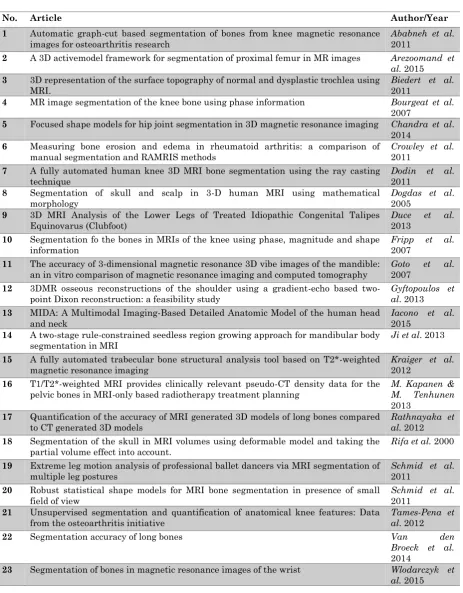
No. Article Author/Year

1 Automatic graph-cut based segmentation of bones from knee magnetic resonance

images for osteoarthritis research Ababneh et al. 2011

2 A 3D activemodel framework for segmentation of proximal femur in MR images Arezoomand et

al. 2015

3 3D representation of the surface topography of normal and dysplastic trochlea using

MRI. Biedert et al. 2011

4 MR image segmentation of the knee bone using phase information Bourgeat et al.

2007

5 Focused shape models for hip joint segmentation in 3D magnetic resonance imaging Chandra et al.

2014

6 Measuring bone erosion and edema in rheumatoid arthritis: a comparison of

manual segmentation and RAMRIS methods Crowley et al. 2011

7 A fully automated human knee 3D MRI bone segmentation using the ray casting

technique

Dodin et al.

2011

8 Segmentation of skull and scalp in 3-D human MRI using mathematical

morphology Dogdas et al. 2005

9 3D MRI Analysis of the Lower Legs of Treated Idiopathic Congenital Talipes

Equinovarus (Clubfoot) Duce et al. 2013

10 Segmentation fo the bones in MRIs of the knee using phase, magnitude and shape

information Fripp et al. 2007

11 The accuracy of 3-dimensional magnetic resonance 3D vibe images of the mandible:

an in vitro comparison of magnetic resonance imaging and computed tomography Goto 2007 et al.

12 3DMR osseous reconstructions of the shoulder using a gradient-echo based

two-point Dixon reconstruction: a feasibility study Gyftopoulos et al. 2013

13 MIDA: A Multimodal Imaging-Based Detailed Anatomic Model of the human head

and neck Iacono et al. 2015

14 A two-stage rule-constrained seedless region growing approach for mandibular body

segmentation in MRI Ji et al. 2013

15 A fully automated trabecular bone structural analysis tool based on T2*-weighted

magnetic resonance imaging Kraiger et al. 2012

16 T1/T2*-weighted MRI provides clinically relevant pseudo-CT density data for the pelvic bones in MRI-only based radiotherapy treatment planning

M. Kapanen & M. Tenhunen

2013

17 Quantification of the accuracy of MRI generated 3D models of long bones compared

to CT generated 3D models Rathnayaka et al. 2012

18 Segmentation of the skull in MRI volumes using deformable model and taking the

partial volume effect into account. Rifa et al. 2000

19 Extreme leg motion analysis of professional ballet dancers via MRI segmentation of

multiple leg postures

Schmid et al.

2011 20 Robust statistical shape models for MRI bone segmentation in presence of small

field of view

Schmid et al.

2011

21 Unsupervised segmentation and quantification of anatomical knee features: Data

from the osteoarthritis initiative

Tames-Pena et al. 2012

22 Segmentation accuracy of long bones Van den

Broeck et al.

2014

23 Segmentation of bones in magnetic resonance images of the wrist Wlodarczyk et

Appendix B

A short explanation of the threshold and region growing method in Mimics Medical 18.0 is described in this appendix.

The thresholding method uses a threshold value or a range of grey values to make a mask. The threshold value is the cut-off value: pixels below the value are included in the mask and pixels above the threshold value are excluded from the mask. In this study, the threshold was based on visual check of the mask in the axial, coronal and/or sagittal slices. After selecting the optimal threshold range, the structures that did not belong to the mandible were manually removed using the ‘edit mask’ and/or ‘multiple slice edit’ tool. This includes structures as teeth and other surrounding structures. To get rid of separate parts in the mask, the ‘region growing’ tool was used. After these steps, the mask was translated into a 3D model by using the ‘calculate 3D from mask’ tool with optimal settings. The optimal settings for smoothing of the 3D model were tested. Therefore, different smoothing factors and the number of iterations were varied. The influence of the checkbox ‘compensate shrinking on’ was also evaluated. The optimal settings were selected by visually choose the 3D model where the contours matched the most with the unsmoothed model, but where the surfaces where smoothed.

Appendix C

The influence of smoothing on the segmentation is explored. This appendix shows the results.

Figure C-1 shows a zoomed view of an axial slice of one of the black bone scans. The black line is the contour of the mandible. The coloured contours represent the outline of equal 3D models of the mandible obtained by thresholding and manual editing. Differences are seen due to smoothing settings calculating a 3D model from the mask. The pink line is the contour of the unsmoothed 3D model. The blue line represents the contour of the (pink) 3D model smoothed during 3D model calculation. The green line is the contour of the (pink) 3D model smoothed after 3D model calculation with the following settings: iterations 5, smooth factor 0.8, compensate shrinking on. Figure C-2 shows the corresponding 3D models. The initial model (pink) needs smoothing to get rid of the rough surface. The blue model shows a smooth surface. However, this model overestimates the shape of the mandible, as can be seen in Figure C-1 showing the overestimated, larger blue contour. The green 3D model has a smooth surface and, unlike the green model, the contour follows the pink contour. These images shows that smoothing with the defined settings (iterations 5, smoothing factor 0.8, and compensate shrinking on) does not over- or underestimate the shape of the mandible, while obtaining a smooth model.

Figure C-1 Axial slice of a black bone scan showing different contours of 3D models caused by different smoothing

Figure C-2 Example 3D models of the broad exploration phase showing the influence of different smoothing settings.

Appendix D

This appendix contains the results of the broad exploration of MRI sequences. Per evaluated sequence, a 3D model of the segmentation result and screenshots of coronal, axial and sagittal slices are given. The list of requirements including explanation is also attached to this appendix.

TABLE D-1 Characteristics of the 8 evaluated sequences of the broad exploration phase

Sequence Pixel size (mm2₎

Slice thickness (mm)

Acquisition

time (min) Comments Figure

T1 3D VIBE 1.0 1.0 06:34 Segmentation n/a, cadaver _scan T1-weighted 3D

Dixon VIBE in phase 0.7 0.7 06:23 Promising segmentation Figure D-1 T1-weighted 3D

StarVIBE 0.9 2.0 02:53

Segmentation difficulties due to 2.0 mm slice thickness, a lot of manual editing

Figure D-2 T1-weighted 3D

MPRAGE 1.0 1.0 05:24 Segmentation n/a, cadaver scan T1-weighted TSE 0.7 3.0 01:24*2 Bad segmentation quality, due to 3.0 mm slice thickness

Figure D-3 T2-weighted 3D

FLAIR + FATSAT 1.0 1.0 05:55 Tolerable quality, noisy segmentation Figure D-4

T2-weighted Blade 0.6 3.0 01:31*2 Bad segmentation quality due to bad resolution in coronal and sagittal slices

Figure D-5

3D black bone VIBE 0.5 1.0 06:50 Promising segmentation Figure _D-6

D.1 Dixon VIBE

Figure D-1 Coronal, axial and sagittal slices and 3D model reconstruction of the mandible segmentation of a T1-weighted

D.2 StarVIBE

Figure D-2 A Coronal, axial and sagittal slices (left to right) of a T1-weighted starVIBE sequence. B 3D model of the

mandible segmented from a T1-weighted starVIBE sequence (orange) with the CT model (transparent). C Colour map showing the deviation between MRI- and CT-based model of a T1-weighted starVIBE sequence. The colour scale is from minus 6.0 mm (blue) to 6.0 mm (red).

D.3 TSE

Figure D-3 Coronal, axial and sagittal slices (left to right) and 3D model reconstruction of segmented mandible of a

T1-weighted TSE sequence. A

D.4 FLAIR

Figure D-4 Coronal, axial and sagittal slices (left to right) and 3D model reconstruction of mandible segmentation of a

T2-weighted FLAIR + FATSAT sequence.

D.5 BLADE

Figure D-5 Coronal, axial and sagittal slices (left to right) and 3D model reconstruction of a mandible segmentation of a

D.6 Black bone

Figure D-6 A Coronal, axial and sagittal slices (left to right) of a black bone VIBE sequence showing the mandible. B 3D

model of the segmented mandible from a black bone VIBE sequence. C Colour map showing the deviation between the MRI- and CT-based model of the segmented mandible from a black bone VIBE sequence.

Table D-2 List of requirements for MRI sequence and settings and segmentation method based on the broad exploration

of MRI sequences, settings and segmentations.

Requirements for MRI sequence and settings:

1. Contrast between bone and surrounding tissue

2. Executable in 3 Tesla MRI scanner

3. Isotropic voxel size ≤ 1mm

4. 3D acquisition

5. Mandible in field of view

6. Acquisition time ≤ 10 minutes

Requirements for the segmentation method:

7. Segmentation time ≤ 1 hour

8. Software available in the hospital

9. Maximal deviation from ‘gold standard’ at critical sites ≤ 1mm

10. No fusion of different imaging modalities

11. Result is an 3D STL file

12. Compatible with MRI data

13. Applicable in all individual cases

3.000

2.103

1.207

0.310

-0.310

1.207

2.103

3.000

A

The structure that need to be segmented must be visible in the MRI data. Therefore, as high as possible contrast between bone and surrounding tissue is desirable. The workflow must fit in the daily practice, thus the sequence must be executed in the MRI scanner used for all head and neck patients (3 Tesla MRI scanner). Based on the segmentations made in the broad exploration phase, a isotropic voxel size benefits the segmentation result. Moreover, the voxel size needs to be equal to or smaller than 1 mm for proper 3D modelling comparable to 3D CT-based models. To obtain the small voxel size of 1 mm or smaller, 3D acquisition is necessary. The mandible need to be in the field of view to segment this structure properly. The total acquisition time need to be as low as possible, to avoid movement artefacts and to maintain patient comfort. Moreover, to fit the new workflow in the daily practise, the additional scanning time must be restricted to 10 minutes.

Appendix E

This appendix includes the results of the test series of this study. The settings and characteristics of the sequences are elaborated and images showing metal artefacts are added.

Table E-1 Sequences and characteristics of the sequences performed in the test series

No. Series description FA BW TR TE TA Volunteer

1 Standard 2 210 6.2 2.53 2:34 1,2,3

2 Standard 3 210 6.2 2.53 2:34 1,2

3 Out of phase 5 500 3.78 1.54 1:34 1,2,3

4 With quick FATSAT 5 210 6.11 2.5 2:39 1,2,3

5 Standard 5 210 6.11 2.5 2:32 1,2,3

6 Without interpolation 5 210 6.2 2.53 4:13 1,2

7 Standard 7 210 6.2 2.53 2:34 1,2

8 Without interpolation + GRAPPA 5 210 6.2 2.52 3:28 2

9 Out of phase + GRAPPA 2 500 3.78 1.54 1:20 3

10 Out of phase + GRAPPA3 2 500 3.78 1.54 58.37 3

11 Out of phase 2 500 3.78 1.54 2:26 3

12 With quick FATSAT 2 210 6.11 2.5 4:05 3

13 With quick FATSAT + GRAPPA 2 210 6.11 2.5 2:14 3

14 With quick FATSAT + GRAPPA3 2 210 6.11 2.5 1:37 3

15 With GRAPPA 3 2 210 6.11 2.5 1:34 3

16 Out of phase + GRAPPA 5 500 3.78 1.54 1:20 3

17 With quick FATSAT +GRAPPA 5 210 6.11 2.5 2:14 3

FA = flip angle (degree), BW = pixel bandwidth (Hz/pixel), TR = Repetition time (ms), TE = Echo time (ms), TA = acquisition time (min)

Figure E-1 A Axial view of a black bone out of phase scan (flip angle = 2°) showing artefacts caused by a metal splint on

the upper dentition. B Axial view of a standard black bone scan (flip angle = 2°) with quick FATSAT showing the same metal artefact.

Appendix F

This appendix contains images of the results of the MRI-based surgery section of this thesis.

Figure F-1 MRI-based 3D mandible models utilised for MRI-based guided surgery. Left: case 1, derived from black bone

with quick FATSAT + GRAPPA and a flip angle of 2°. Right: case 2, derived from black bone with flip angle of 2°.

Figure F-2 Virtual CT-based mandible model with test plate designed on MRI. The plate shows small deviations from the