Canonical correlation analysis; An overview with application to learning methods

Canonical correlation analysis; An

overview with application to learning

methods

David R. Hardoon , Sandor Szedmak and John Shawe-Taylor

Department of Computer Science

Royal Holloway, University of London

{

davidh, sandor, john

}

@cs.rhul.ac.uk

Technical Report

CSD-TR-03-02

May 28, 2003

We present a general method using kernel Canonical Correlation Analysis to learn a semantic representation to web images and their associated text. The semantic space provides a common representation and enables a comparison between the text and images. In the experiments we look at two approaches of retrieving images based only on their content from a text query. We com-pare the approaches against a standard cross-representation retrieval technique known as the Generalised Vector Space Model.

Introduction 1

1

Introduction

During recent years there have been advances in data learning using kernel methods. Kernel representation offers an alternative learning to non-linear functions by projecting the data into a high dimensional feature space to increase the computational power of the linear learning machines, though this still leaves open the issue of how best to choose the features or the kernel func-tion in ways that will improve performance. We review some of the methods that have been developed for learning the feature space.

• Principal Component Analysis (PCA) is a multivariate data analysis proce-dure that involves a transformation of a number of possibly correlated variables into a smaller number of uncorrelated variables known as principal components. PCA only makes use of the training inputs while making no use of the labels.

• Independent Component Analysis (ICA) in contrast to correlation-based transformations such as PCA not only decorrelates the signals but also reduces higher-order statistical dependencies, attempting to make the signals as inde-pendent as possible. In other words, ICA is a way of finding a linear not only orthogonal co-ordinate system in any multivariate data. The directions of the axes of this co-ordinate system are determined by both the second and higher order statistics of the original data. The goal is to perform a linear transform which makes the resulting variables as statistically independent from each other as possible.

• Partial Least Squares (PLS) is a method similar to canonical correlation analysis. It selects feature directions that are useful for the task at hand, though PLS only uses one view of an object and the label as the corresponding pair. PLS could be thought of as a method, which looks for directions that are good at distinguishing the different labels.

• Canonical Correlation Analysis (CCA) is a method of correlating linear relationships between two multidimensional variables. CCA can be seen as us-ing complex labels as a way of guidus-ing feature selection towards the underlus-ing semantics. CCA makes use of two views of the same semantic object to extract the representation of the semantics. The main difference between CCA and the other three methods is that CCA is closely related to mutual information (Borga 1998 [3]). Hence CCA can be easily motivated in information based tasks and is our natural selection.

During recent years there has been a vast increase in the amount of mul-timedia content available both off-line and online, though we are unable to access or make use of this data unless it is organised in such a way as to allow efficient browsing. To enable content based retrieval with no reference to labeling we attempt to learn the semantic representation of images and their associated text. We present a general approach using KCCA that can be used for content [11] to as well as mate based retrieval [18, 11]. In both cases we compare the KCCA approach to the Generalised Vector Space Model (GVSM), which aims at capturing some term-term correlations by looking at co-occurrence information.

This study aims to serve as a tutorial and give additional novel contribu-tions in the following ways:

• In this study we follow the work of Borga [4] where we represent the eigenproblem as two eigenvalue equations as this allows us to reduce the com-putation time and dimensionality of the eigenvectors.

• Further to that, we follow the idea of Bach & Jordan [2] to compute a new correlation matrix with reduced dimensionality. Though Bach & Jordan [2] address a very different problem, they use the same underlining technique of Cholesky decomposition to re-represent the kernel matrices. We show that by using partial Gram-Schmidt orthogonolisation [6] is equivalent to incomplete Cholesky decomposition, in the sense that incomplete Cholesky decomposition can be seen as a dual implementation of partial Gram-Schmidt.

• We show that the general approach can be adapted to two different types of problems, content and mate retrieval, by only changing the selection of eigenvectors used in the semantic projection.

• To simplify the learning of the KCCA we explore a method of selecting the regularization parameter a priori such that it gives a value that performs well in several different tasks.

In this study we also present a generalisation of the framework for canoni-cal correlation analysis. Our approach is based on the works of Gifi (1990) and Ketterling (1971). The purpose of the generalisation is to extend the canonical correlation as an associativity measure between two set of variables to more than two sets, whilst preserving most of its properties. The generalisation starts with the optimisation problem formulation of canonical correlation. By changing the objective function we will arrive at the multi set problem. Ap-plying similar constraint sets in the optimisation problems we find that the feasible solutions are singular vectors of matrices, which are derived the same way for the original and generalised problem.

Theoretical Foundations 3

we present the CCA and KCCA algorithm. Approaches to deal with the com-putational problems that arose in Section 3 are presented in Section 4. Our experimental results are presented In Section 5. In Section 6 we present the generalisation framework for CCA while in Section 7 draws final conclusions.

2

Theoretical Foundations

Proposed by H. Hotelling in 1936 [12], Canonical correlation analysis can be seen as the problem of finding basis vectors for two sets of variables such that the correlation between the projections of the variables onto these basis vectors are mutually maximised. Correlation analysis is dependent on the co-ordinate system in which the variables are described, so even if there is a very strong linear relationship between two sets of multidimensional variables, depending on the co-ordinate system used, this relationship might not be visible as a cor-relation. Canonical correlation analysis seeks a pair of linear transformations one for each of the sets of variables such that when the set of variables are transformed the corresponding co-ordinates are maximally correlated.

Consider a multivariate random vector of the form (x,y). Suppose we are given a sample of instances S = ((x1,y1), . . . ,(xn,yn)) of (x,y), we use Sx to denote (x1, . . . ,xn) and similarly Sy to denote (y1, . . . ,yn). We can consider

defining a new co-ordinate for x by choosing a direction wx and projecting x onto that direction

x_{→ h}wx,xi

if we do the same fory by choosing a directionwy we obtain a sample of the newx co-ordinate as

Sx,wx = (hwx,x1i, . . . ,hwx,xni)

with the corresponding values of the newy co-ordinate being

Sy,wy = (hwy,y1i, . . . ,hwy,yni)

The first stage of canonical correlation is to choose wx and wy to maximise the correlation between the two vectors. In other words the function to be maximised is

ρ = max

wx,wy

corr(Sxwx, Sywy)

= max

wx,wy

hSxwx, Sywyi

kSxwxkkSywyk

If we use ˆE[f(x,y)] to denote the empirical expectation of the functionf(x,y), were

ˆ

E[f(x,y)] = 1

m

m

X

i=1

we can rewrite the correlation expression as

ρ = max

wx,wy

ˆ

E[_hwx,xihwy,yi]

q

ˆ

E[_hwx,xi2]ˆE[hwx,xi2]

= max

wx,wy

ˆ

E[w0_xxy0wy]

q

ˆ E[w0

xxx0wx]ˆE[w0yyy0wy]

follows that

ρ= max

wx,wy

w0_xEˆ[xy0]wy

q

w0

xEˆ[xx0]wxw0yEˆ[yy0]wy

.

Where we useA0 _{to denote the transpose of a vector or matrix A.}

Now observe that the covariance matrix of (x,y) is

C(x,y) = ˆE

"

x y

x y

0#

=

Cxx Cxy

Cyx Cyy

=C. (2.1)

The total covariance matrix C is a block matrix where the within-sets covari-ance matrices are Cxx and Cyy and the between-sets covariance matrices are

Cxy =Cyx0

Hence, we can rewrite the functionρ as

ρ = max

wx,wy

w0_xCxywy

p

w0

xCxxwxw0yCyywy

(2.2)

the maximum canonical correlation is the maximum of ρ with respect to wx andwy.

3

Algorithm

In this section we will give an overview of the Canonical correlation analysis (CCA) and Kernel-CCA (KCCA) algorithms where we formulate the optimisa-tion problem as a generalised eigenproblem.

3.1

Canonical Correlation Analysis

Observe that the solution of equation (2.2) is not affected by re-scalingwx or

wy either together or independently, so that for example replacing wx byαwx gives the quotient

αw0_xCxywy

q α2_w0

xCxxwxw0yCyywy

= w

0

xCxywy

p

w0

xCxxwxw0yCyywy

.

Algorithm 5

subject to

w0_xCxxwx = 1 w0_yCyywy = 1.

The corresponding Lagrangian is

L(λ,wx,wy) =w0xCxywy−

λx 2 (w

0

xCxxwx−1)−

λy 2 (w

0

yCyywy−1)

Taking derivatives in respect towx and wy we obtain

∂f ∂wx

=Cxywy−λxCxxwx= 0 (3.1)

∂f ∂wy

=Cyxwx−λyCyywy = 0. (3.2)

Subtractingw_y0 times the second equation fromw0_x times the first we have

0 = w0_xCxywy−w0xλxCxxwx−w0yCyxwx+w0yλyCyywy = λyw0yCyywy−λxw

0

xCxxwx,

which together with the constraints implies thatλy−λx = 0, letλ=λx=λy. AssumingCyy is invertible we have

wy =

C_yy−1Cyxwx

λ (3.3)

and so substituting in equation (3.1) gives

CxyC

−1

yyCyxwx

λ −λCxxwx = 0

or

CxyC

−1

yyCyxwx = λ

2_C

xxwx (3.4)

We are left with a generalised eigenproblem of the form Ax =λBx. We can therefore find the co-ordinate system that optimises the correlation between corresponding co-ordinates by first solving for the generalised eigenvectors of equation (3.4) to obtain the sequence ofwx’s and then using equation (3.3) to find the correspondingwy’s.

As the covariance matrices Cxx and Cyy are symmetric positive definite

we are able to decompose them using a complete Cholesky decomposition (more details on Cholesky decomposition can be found in section 4.2)

Cxx=Rxx·R

0

xx

whereRxx is a lower triangular matrix. If we letux =R0xx·wx we are able to

rewrite equation (3.4) as follows

CxyC

−1

yyCyxR

−10

xx ux = λ

2_R

xxux

R−_xx1CxyC

−1

yyCyxR

−10

xx ux = λ

2_u

x.

3.2

Kernel Canonical Correlation Analysis

CCA may not extract useful descriptors of the data because of its linearity. Kernel CCA offers an alternative solution by first projecting the data into a higher dimensional feature space

φ:x= (x1, . . .xn)7→φ(x) = (φ1(x), . . . , φN(x)) (n < N)

before performing CCA in the new feature space, essentially moving from the primal to the dual representation approach. Kernels are methods of implicitly mapping data into a higher dimensional feature space, a method known as the ”kernel trick”. A kernel is a functionK, such that for allx, z _∈X

K(x, z) =< φ(x)_·φ(z)> (3.5) whereφ is a mapping fromX to a feature space F. Kernels offer a great deal of flexibility, as they can be generated from other kernels. In the kernel the data only appears through entries in the Gram matrix, therefore this approach gives a further advantage as the number of tuneable parameters and updating time does not depend on the number of attributes being used.

Using the definition of the covariance matrix in equation (2.1) we can rewrite the covariance matrixC using the data matrices (of vectors) X and Y, which have the sample vector as rows and are therefore of sizem_×N, we obtain

Cxx = X0X

Cxy = X

0_Y.

The directionswx and wy (of lengthN) can be rewritten as the projection of the data onto the directionα and β (of length m)

wx = X0α

wy = Y0β.

Substituting into equation (2.2) we obtain the following

ρ = max

α,β

α0XX0Y Y0β

√

α0_XX0_XX0_α·β0_{Y Y}0_{Y Y}0_β (3.6)

LetKx =XX0 andKy =Y Y0 be the kernel matrices corresponding to the two representation. We substitute into equation (3.6)

ρ = max

α,β

α0KxKyβ

q α0_K2

xα·β0Ky2β

. (3.7)

We find that in equation (3.7) the variables are now represented in the dual form.

Algorithm 7

the KCCA optimisation problem formulated in equation (3.7) is equivalent to maximising the numerator subject to

α0K_x2α = 1

β0K_y2β = 1 The corresponding Lagrangian is

L(λ, α, β) =α0KxKyβ−

λα

2 α

0_K2

xα−1

−λ₂β β0K_y2β₋1

Taking derivatives in respect toα and β we obtain

∂f

∂α =KxKyβ−λαK

2

xα= 0 (3.8)

∂f

∂β =KyKxα−λβK

2

yβ = 0. (3.9)

Subtractingβ0 _{times the second equation from α}0 _{times the first we have}

0 = α0KxKyβ−α0λαKx2α−β0KyKxα+β0λβKy2β = λββ0Ky2β−λαα0Kx2α

which together with the constraints implies thatλα−λβ = 0, let λ=λα=λβ. Considering the case where the kernel matrices Kx and Ky are invertible, we have

β = K

−1

y Ky−1KyKxα

λ

= K

−1

y Kxα

λ

substituting in equation (3.8) we obtain

KxKyKy−1Kxα−λ2KxKxα = 0. Hence

KxKxα−λ2KxKxα= 0 or

Iα=λ2

α. (3.10)

We are left with a generalised eigenproblem of the form Ax = λx. We can deduce from equation 3.10 that λ = 1 for every vector of α; hence we can choose the projections wx to be unit vectors ji i= 1, . . . , m while wy are the columns of 1_λK−1

4

Computational Issues

We observe from equation (3.10) that ifKx is invertible maximal correlation is obtained, suggesting learning is trivial. To force non-trivial learning we intro-duce a control on the flexibility of the projections by penalising the norms of the associated weight vectors by a convex combination of constraints based on Partial Least Squares. Another computational issue that can arise is the use of large training sets, as this can lead to computational problems and degener-acy. To overcome this issue we apply partial Gram-Schmidt orthogonolisation (equivalently incomplete Cholesky decomposition) to reduce the dimensionality of the kernel matrices.

4.1

Regularisation

To force non-trivial learning on the correlation we introduce a control on the flexibility of the projection mappings using Partial Least Squares (PLS) to penalise the norms of the associated weights. We convexly combine the PLS term with the KCCA term in the denominator of equation (3.7) obtaining

ρ = maxα,β α

0_K

xKyβ

q

(α0_K2

xα+κkwxk2)·(β0Ky2β+κkwyk2))

= maxα,β α

0_K

xKyβ

q

(α0_K2

xα+κα0Kxα)·(β0Ky2β+κβ0Kyβ)

.

We observe that the new regularised equation is not affected by re-scaling ofα

orβ, hence the optimisation problem is subject to (α0K_x2α+κα0Kxα) = 1

(β0K_y2β+κβ0Kyβ) = 1 The corresponding Lagrangain is

L(λα, λβ, α, β) = α0KxKyβ

−λ₂α(α0K_x2α+κα0Kxα−1)

−λ₂β(β0Ky2β+κβ0Kyβ−1).

Taking derivatives in respect toα and β ∂f

∂α = KxKyβ−λα(K

2

xα+κKxα) (4.1)

∂f

∂β = KyKxα−λβ(K

2

yβ+κKyβ). (4.2)

Subtractingβ0 times the second equation from α0 times the first we have 0 = α0KxKyβ−λαα0(Kx2α+κKxα)−β0KyKxα+λββ0(Ky2β+κKyβ)

Computational Issues 9

Which together with the constraints implies thatλα−λβ = 0, letλ=λα=λβ. Consider the case whereKx and Ky are invertible, we have

β = (Ky+κI)

−1_K−1

y KyKxα

λ

= (Ky+κI)

−1_K

xα

λ

substituting in equation 4.1 gives

KxKy(Ky+κI)−1Kxα = λ2Kx(Kx+κI)α

Ky(Ky+κI)−1Kxα = λ2(Kx+κI)α (Kx+κI)−1Ky(Ky+κI)−1Kxα = λ2α

We obtain a generalised eigenproblem of the formAx=λx .

4.2

Cholesky Decomposition

We describe some background information on direct factorisation methods on triangular decomposition [13].

LU =A (4.3)

in which the diagonal elements of L are not necessarily unity. We consider

L_≡(lij) then equation (4.3) implies

lkkukk = akk− k−1

X

p=1

lkpupk fork≥2 (4.4)

ukj = 1

lkk



akj− k−1

X

p=1

lkpupj



 forj > k≥2 (4.5)

lik = 1

ukk



aik− k−1

X

p=1

lipupk



 fori > k≥2 (4.6)

Theorem 1. Let A be symmetric. If the factorisation LU = A is possible, then the choicelkk =ukk implies lik=uki, that is, LLT =A.

Proof. Use equation (4.4) and induction on k.

A simple, non-singular, symmetric matrix for which the factorisation is not possible is

0 1 1 0

Theorem 2. Let A be symmetric, positive definite. Then,A can be factored in the form

LL0 =A

Proof. If we definelkk=ukk=√bkk then we will obtain from the previous equationsLU =A wherelik=uki

Incomplete Cholesky Decomposition

Complete decomposition of a kernel matrix is an expensive step and should be avoided with real world data. Incomplete Cholesky decomposition as described in [2] differs from Cholesky decomposition in that all pivots, which are below a certain threshold are skipped. If M is the number of non-skipped pivots, then we obtain a lower triangular matrix Gi _{with only M nonzero columns.} Symmetric permutations of rows and columns are necessary during the factori-sation if we require the rank to be as small as possible (Golub and loan, 1983).

We describe the algorithm from [2] (with slight modification) :

InputN xN matrixK

precision parameterη

1. Initialisation: i= 1, K0_{=K,P =I, forj∈[1, N], G}

jj =Kjj 2. WhilePN

j=1Gjj > η and i! =N + 1

• Find best new element: j∗=argmaxj∈[i,N]Gjj

• Updatej∗ = (j∗+i)₋1

• Update permutation P :

P next=I,P nextii= 0,P nextj∗_j∗ = 0,P next_ij∗= 1, P next_j∗_i= 1

P =P_·P next

• Permute elementsiand j∗ _inK0_: K0 _{=P next·K}0_{·P next}

• Update (due to new permutation) the already calculated elements of G: Gi,1:i−1↔Gj∗,1:i−1

• Permute elementsj∗_{, j}∗ _{andi, i of G:} G(i, i)_↔G(j∗, j∗)

• SetGii=√Gii

• Calculateith column of G:

Gi+1:n,i= _G1_ii

K_i0_+1:n,i−Pi−1

j=1Gi+1:n,jGij

•Update only diagonal elements: for j_∈[i+ 1, N], Gjj =Kjj0 −

Pi

k=1G2jk

• Updatei=i+ 1 3. OutputP,Gand M =i

Output: an N _×M lower triangular matrix G and a permutation matrix

P such that_kP0KP ₋GG0_{k ≤}η (appendix 1.2 for proof).

Computational Issues 11

in the error of the approximation. After l steps, we have an approximation of the form ˜Kl = Gi_lG0il, where Gil is N ×l. The ranking of the N −l vectors can be computed by comparing the diagonal elements of the remainder matrix

K₋Gi_lG0il.

Partial Gram-Schmidt Orthogonolisation

We explore the Partial Gram-Schmidt Orthogonolisation (PGSO) algorithm, described in [6], as our matrix decomposition approach. ICD could been as equivalent to PGSO as ICD is the dual implementation of PGSO. PGSO works as follows; The projection is built up as the span of a subset of the projections of a set ofm training examples. These are selected by performing a Gram-Schmidt orthogonalisation of the training vectors in the feature space. We slightly modify the Gram-Schmidt algorithm so it will use a precision parameter as a stopping criterion as shown in [2].

Given a kernelK from a training set, and precision parameter η:

Initialisations:

m= size of K, aN _×N matrix

j= 1

size and indexare a vector with the same length as K f eata zeros matrix equal to the size of K

fori= 1 to m do norm2[i] =Kii;

Algorithm:

while P

inorm2[i]> η and j! =N+ 1 do

ij =argmaxi(norm2[i]); index[j] =ij;

size[j] =pnorm2[ij]; fori= 1 to mdo

feat[i, j] =

“

k(di,d_ij)−Ptj=1−1f eat[i,t]·f eat[ij,t] ”

size[j] ;

norm2[i] = norm2[i]₋feat(i, j)_· feat(i, j); end;

j =j+ 1 end;

return feat

Output:

kK ₋f eat_·f eat0_{k ≤} η where f eat is a N _×M lower triangular matrix (appendix 1.2 for proof)

We observe that the output is equivalent to the output of ICD.

Given a kernelK from a testing set

forj= 1 to M

newfeat[j] = (Ki,index[j]−Pjt=1−1 newfeat[t]·feat[index[j], t])/size[j];

end;

The advantage of using the partial Gram-Schmidt orthonogolisation (PGSO) in comparison to the incomplete Cholesky decomposition (as described in Section 4.2) is that there is no need for a permutation matrixP.

4.3

Kernel-CCA with PGSO

So far we have considered the kernel matrices as invertible, although in prac-tice this may not be the case. In this Section we address the issue of using large training sets, which may lead to computational problems and degeneracy. We use PGSO to approximate the kernel matrices such that we are able to re-represent the correlation with reduced dimensiality.

Decomposing the kernel matrices Kx and Ky via PGSO, where R is a lower triangular matrix, gives

Kx =˜ RxR0x

Ky =˜ RyRy0

substituting the new representation into equations (3.8) and (3.9)

RxR0xRyR0yβ−λRxR0xRxR0xα = 0 (4.7)

RyR0yRxR0xα−λRyR0yRyR0yβ = 0. (4.8) Multiplying the first equation withR0

x and the second equation withR0y gives

R0_xRxR0xRyR0yβ−λRx0RxR0xRxRx0α = 0 (4.9)

R0_yRyR0yRxR0xα−λR0yRyR0yRyRy0β = 0. (4.10) LetZ be the new correlation matrix with the reduced dimensiality

R0_xRx = Zxx

R0yRy = Zyy

R_x0Ry = Zxy

R_y0Rx = Zyx Let ˜α and ˜β be the reduced directions, such that

˜

α = R0_xα

˜

β = R0_yβ

substituting in equations (4.9) and (4.10) we find that we return to the primal representation of CCA with a dual representation of the data

ZxxZxyβ˜−λZxx2 α˜ = 0

Computational Issues 13

Assuming that the Zxx and Zyy are invertible. We multiply the first equation withZ_xx−1 and the second withZ_yy−1

Zxyβ˜−λZxxα˜ = 0 (4.11)

Zyxα˜−λZyyβ˜ = 0. (4.12)

We are able to rewrite ˜β from equation (4.12) as

˜

β =Z

−1

yyZyxα˜

λ

and substituting in equation (4.11) gives

ZxyZyy−1Zyxα˜ = λ2Zxxα˜ (4.13) we are left with a generalised eigenproblem of the form Ax = λBx. Let SS0

be equal to the complete Cholesky decomposition ofZxx such that Zxx =SS0 whereSis a lower triangular matrix, and let ˆα=S0_·α˜. Substituting in equation (4.13) we obtain

S−1ZxyZyy−1ZyxS−1

0

ˆ

α = λ2αˆ

We now have a symmetric generalised eigenproblem of the formAx=λx.

KCCA Regularisation with PGSO

We combine the dimensiality reduction introduced in the previous Section 4.3 with the regularisation parameter (Section 4.1) to maximise the learning. Fol-lowing the same approach in the previous section we can rewrite equations (4.1) and (4.2) with the approximation ofKxandKy as formulated in equations (4.7) and (4.8) respectively, in the following manner

RxRx0RyR0yβ−λ(RxR0xRxRx0 +κRxR0x)α = 0

RyR0yRxR0xα−λ(RyRy0RyR0y+κRyRy0)β = 0 Multiplying the first equation withR0

x and the second equation withR0y gives

R0_xRxRx0RyR0yβ−λR0x(RxR0xRxR0x+κRxR0x)α = 0 (4.14)

R0_yRyR0yRxR0xα−λR0y(RyR0yRyR0y+κRyR0y)β = 0 (4.15) rewriting equation (4.14) with the new reduced correlation matrixZ as defined in the previous Section 4.3, we obtain

ZxxZxyβ˜−λZxx(Zxx+κI)˜α = 0

ZyyZyxα˜−λZyy(Zyy+κI) ˜β = 0.

Assuming that the Zxx and Zyy are invertible. We multiply the first equation withZ_xx−1 and the second withZ_yy−1

Zxyβ˜−λ(Zxx+κI)˜α = 0 (4.16)

We are able to rewrite ˜β from equation (4.17) as

˜

β = (Zyy+κI)

−1_Z

yxα˜

λ

substituting in equation 4.16 gives

Zxy(Zyy+κI)−1Zyxα˜ =λ2(Zxx+κI)˜α

We are left with a generalised eigenproblem of the formAx=λBx. Performing a complete Cholesky decomposition on Zxx +κI = SS0 where S is a lower triangular matrix. and let ˆα=S0α˜, substituting in equation (4.18)

S−1Zxy(Zyy+κI)−1ZyxS−1

0

ˆ

α = λ2α.ˆ

We obtain a symmetric generalised eigenproblem of the formAx=λx.

5

Experimental Results

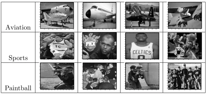
In the following experiments the problem of learning semantics of multimedia content by combining image and text data is addressed. The synthesis is ad-dressed by the kernel Canonical correlation analysis described in Section 4.3. We test the use of the derived semantic space in an image retrieval task that uses only image content. The aim is to allow retrieval of images from a text query but without reference to any labeling associated with the image. This can be viewed as a cross-modal retrieval task. We used the combined multime-dia image-text web database, which was kindly provided by the authors of [15], where we are trying to facilitate mate retrieval on a test set. The data was di-vided into three classes (Figure 1) - Sport, Aviation and Paintball - 400 records each and consisted of jpeg images retrieved from the Internet with attached text. We randomly split each class into two halves which were used as training and test data accordingly. The extracted features of the data were used the same as in [15] (detailed description of the features used can be found in [15]: image HSV colour, image Gabor texture and term frequencies in text.

Experimental Results 15

Aviation 50 100 150 200 250 300 350 400 20 40 60 80 100 120 140 160 180 200

50 100150200250300350400450500 20 40 60 80 100 120 140 160 180 200

50 100 150 200 250 300 350 400 20 40 60 80 100 120 140 160 180 200

50 100 150 200250 300 350400 450 20 40 60 80 100 120 140 160 180 200

Sports 10 20 30 40 50 60 70 80 20 40 60 80 100 120

20 40 60 80 100 120 10 20 30 40 50 60 70 80 90

10 20 30 40 50 60 70 80 10 20 30 40 50 60 70 80 90 100 110

20 40 60 80 100 120 10 20 30 40 50 60 70 80 90 100

Paintball 102030405060708090100110 20 40 60 80 100 120 140

20 40 60 80 100 120 140 20 40 60 80 100 120

20 40 60 80 100 120 140 10 20 30 40 50 60 70 80 90 100 110

50 100 150 200 250 300 20 40 60 80 100 120 140 160 180 200

Figure 1 Example of images in database.

difference between the spectrum of the randomized set is maximally different (in the two norm) from the true spectrum.

κ=argmax_kλR(κ)−λ(κ)k

We find that κ= 7 and set via a heuristic technique the Gram-Schmidt preci-sion parameter η= 0.5 .

To perform the test image retrieval we compute the features of the images and text query using the Gram-Schmidt algorithm. Once we have obtained the features for the test query (text) and test images we project them into the semantic feature space using ˜β and ˜α (which are computed through training) respectively. Now we can compare them using an inner product of the semantic feature vector. The higher the value of the inner product, the more similar the two objects are. Hence, we retrieve the images whose inner products with the test query are highest.

We compared the performance of our methods with a retrieval technique based on the Generalised Vector Space Model (GVSM). This uses as a seman-tic feature vector the vector of inner products between either a text query and each training label or test image and each training image. For both methods we have used a Gaussian kernel, withσ = max. distance/20, for the image colour component and all experiments were an average of 10 runs. For convenience we separate the content-based and mate-based approaches into the following Subsections 5.1 and 5.2 respectively.

5.1

Content-Based Retrieval

example for set of 5 images).

Image Set GVSM success KCCA success (30) KCCA success (5)

10 78.93% 85% 90.97%

30 76.82% 83.02% 90.69%

Table 1Success cross-results between kernel-cca & generalised vector space.

0 20 40 60 80 100 120 140 160 180 200

60 65 70 75 80 85 90 95

Image Set Size

Success Rate (%)

KCCA (5) KCCA (30) GVSM

Figure 2Success plot for content-based KCCA against GVSM

In Tables 1 and 2 we compare the performance of the kernel-CCA algorithm and generalised vector space model. In Table 1 we present the performance of the methods over 10 and 30 image sets where in Table 2 as plotted in Figure 2 we see the overall performance of the KCCA method against the GVSM for image sets (1₋200), as in the 2000th image set location the maximum of 200_×600 of the same labelled images over all text queries can be retrieved (we only have 200 images per label). The success rate in Table 1 and Figure 2 is computed as follows

success % for image set i=

P600

j=1

Pi

k=1count

j k

i_×600 ×100

wherecountj_k= 1 if the image kin the set is of the same label as the text query present in the set, elsecountj_k= 0. The success rate in Table 2 is computed as above and averaged over all image sets.

Experimental Results 17

10 20 30 40 50 60 70 80

10 20 30 40 50 60 70 80 90 100 110

10 20 30 40 50 60 70 80

10 20 30 40 50 60 70 80 90 100 110

10 20 30 40 50 60 70 80

10 20 30 40 50 60 70 80 90 100 110

10 20 30 40 50 60 70 80

10 20 30 40 50 60 70 80 90 100 110

10 20 30 40 50 60 70 80

10 20 30 40 50 60 70 80 90 100 110

Figure 3 Images retrieved for the text query: ”height: 6-11 weight: 235 lbs position: forward born: september 18, 1968, split, croatia college: none”

Method overall success

GVSM 72.3%

KCCA (30) 79.12%

KCCA (5) 88.25%

Table 2Success rate over all image sets (1₋200).

few eigenvectors. Hence a minimal selection of 5 eigenvectors is sufficient to obtain a high success rate.

5.2

Mate-Based Retrieval

In the experiment we used the first 150 and 30 ˜αeigenvectors and ˜βeigenvectors (corresponding to the largest eigenvalues). We computed the 10 and 30 images for which their semantic feature vector has the closest inner product with the semantic feature vector of the chosen text. A successful match is considered if the image that actually matched the chosen text is contained in this set. We compute the success as the average of 10 runs (Figure 5 - retrieval example for set of 5 images).

Image set GVSM success KCCA success (30) KCCA success (150)

10 8% 17.19% 59.5%

30 19% 32.32% 69%

Table 3Success cross-results between kernel-cca & generalised vector space.

0 5 10 15 20 25 30 35 40 45 50 30

40 50 60 70 80 90

eigenvectors

Overall Success (%)

Figure 4 Content-Based plot of eigenvector selection against overall success (%).

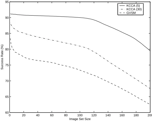
over 10 and 30 image sets where in Table 4 we present the overall success over all image sets. In figure 6 we see the overall performance of the KCCA method against the GVSM for all possible image sets.

The success rate in Table 3 and Figure 6 is computed as follows

success % for image seti=

P600

j=1countj

600 ×100

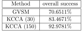
wherecountj = 1 if the exact matching image to the text query was present in the set, else countj = 0. The success rate in Table 4 is computed as above and averaged over all image sets.

Method overall success

GVSM 70.6511%

KCCA (30) 83.4671%

KCCA (150) 92.9781%

Table 4Success rate over all image sets.

Experimental Results 19

50 100 150 200 250 300 350 400 450

20

40

60

80

100

120

140

160

180

200

50 100 150 200 250 300 350 400 450 500 20

40 60 80 100 120 140 160 180 200

20 40 60 80 100 120 140 160 180 200 220

20

40

60

80

100

120

140

20 40 60 80 100 120

10

20

30

40

50

60

70

80

90

50 100 150 200 250 300 350 400 450 500

20

40

60

80

100

120

140

160

180

200

Figure 5 Images retrieved for the text query: ”at phoenix sky harbor on july 6, 1997. 757-2s7, n907wa phoenix suns taxis past n902aw teamwork america west america west 757-2s7, n907wa phoenix suns taxis past n901aw arizona at phoenix sky harbor on july 6, 1997.” The actual match is the middle picture in the first row.

and the reminding eigenvectors would not necessarily add meaningful semantic information.

It is visible that the kernel-CCA significantly outperformes the GVSM method both in content retrieval and in mate retrieval.

5.3

Regularisation Parameter

We next verify that the method of selecting the regularisation parameter κ

a priori gives a value performed well. We randomly split each class into two halves which were used as training and test data accordingly, we keep this divided set for all runs. We set the value of the incomplete Gram-Schmidt orthogonolisation precision parameter η = 0.5 and run over possible values

κ where for each value we test its content-based and mate-based retrieval performance.

Let ˆκbe the previous optimal choice of the regularisation parameter ˆκ=κ= 7. As we define the new optimal value ofκ by its performance on the testing set, we can say that this method is biased (loosely its cheating). Though we will show that despite this, the difference between the performance of the biasedκ

and our a priori ˆκ is slight.

0 100 200 300 400 500 600 0

10 20 30 40 50 60 70 80 90 100

KCCA (150) KCCA (30) GVSM

Figure 6Success plot for KCCA mate-based against GVSM (success (%) against image set size).

κ CB-KCCA (30) CB-KCCA (5)

0 46.278% 43.8374%

ˆ

κ 83.5238% 91.7513%

90 88.4592% 92.7936%

230 88.5548% 92.5281%

Table 5Overall success of Content-Based (CB) KCCA with respect toκ.

performance between the a priori value ˆκ and the new found optimal value

κ for 5 eigenvectors is 1.0423% and for 30 eigenvectors is 5.031%. The more substantial increase in performance on the latter is due to the increase in the selection of the regularisation parameter, which compensates for the substantial decrease in performance (figure 6) of the content based retrieval, when high dimensional semantic feature space is used.

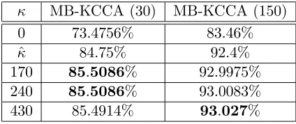
κ MB-KCCA (30) MB-KCCA (150)

0 73.4756% 83.46%

ˆ

κ 84.75% 92.4%

170 85.5086% 92.9975%

240 85.5086% 93.0083%

430 85.4914% 93.027%

Table 6Overall success of Mate-Based (MB) KCCA with respect to κ.

Experimental Results 21

0 20 40 60 80 100 120 140 160 180 50

55 60 65 70 75 80 85 90 95

eigenvectors

overall success (%)

Figure 7Mate-Based plot of eigenvector selection against overall success (%).

100 120 140 160 180 200 220 240 260 280 300 88.4

88.45 88.5 88.55

Kappa

Overall Success (%)

80 85 90 95 100 105 110 115 120 92.778

92.78 92.782 92.784 92.786 92.788 92.79 92.792 92.794 92.796

Overall Success (%)

Kappa

Figure 9 Content-Based. κ selection over overall success for 5 eigenvectors.

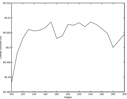
100 120 140 160 180 200 220 240 260 280 300 85.485

85.49 85.495 85.5 85.505 85.51 85.515

Kappa

Overall Success (%)

Generalisation of Canonical Correlation Analysis 23

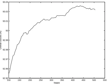
100 150 200 250 300 350 400 450 500 550 92.95

92.96 92.97 92.98 92.99 93 93.01 93.02 93.03

kappa

Overall Succes (%)

Figure 11Mate-Based. κ selection over overall success for 150 eigenvectors.

performance between the a priori value ˆκ and the new found optimal value κ

is for 150 eigenvectors 0.627% and for 30 eigenvectors is 0.7586%.

Our observed results support our proposed method for selecting the regu-larisation parameter κ in an a priori fashion, since the difference between the actual optimalκ and the a priori ˆκ is very slight.

6

Generalisation of Canonical Correlation Analysis

In this section we follow A. Gifi’s book “Nonlinear Multivariate Analysis” (1990) and partially J. R. Ketterling “Canonical analysis of several sets of variables” (1971).

6.1

Some notations

For an n_×n square matrix A having elements _{aij}, i, j = 1, . . . , n we can define the trace by the formula

T r(A) =X i

aii (6.1)

the norm_{k k}F, so called the Frobenius norm, defined by

kA_kF =T r A0A

=X

ij

a2_ij (6.2)

and ifai denotes theithcolumn(row) of A then we have

kA_kF =

X

i

kaik2₂ =

X

i

hai, aii (6.3)

6.2

Some propositions

Proposition 3. Let an optimisation problem be given in the form

min

x,y f(x, y) (6.4)

subject to (6.5)

g(y) = 0, (6.6)

x_∈Rm, y_∈Rn. (6.7)

Let the set Y _⊆ Rn the feasibility domain for y determined by the constrain g(y) = 0.

Assume the functionf is convex in both variablesx andy, the optimal solution of x can be expressed by the function h(y) of the optimal solution of y, where the function of h is defined on the whole set Y and the functions f, g, h are twice continuously differentiable on Rm_×Y.

Then the optimisation problem with the same constrain

min

y f(h(y), y) (6.8)

subject to (6.9)

g(y) = 0, (6.10)

y _∈Rn, (6.11)

has the same optimal solution in y than equation (6.4) has.

Proof. Let the optimal solution of equation (6.4) be denoted by x1, y1 and for

equation (6.8) be denoted byy2.

Based on the condition of the proposition we have x1 = h(y1). Because

y1 is a feasible solution for equation (6.8) thus f(x1, y1) = f(h(y1), y1) ≥

f(h(y2), y2), but the objective function of equation (6.4) is not restricted in

the first variable, thus the inequality f(x1, y1) ≤ f(h(y2), y2) holds, hence

f(x1, y1) =f(h(y2), y2).

From the convexity offand the same feasibility domains the optimum solutions have to be the same.

6.3

Formulation of the Canonical Correlation

Let H(1), H(2) be matrices with size m_×n1, m×n2 respectively and assume

the sum of the elements in the columns of these matrices are equal to 0, they are centralised and they are linearly independent vectors within one matrix. We consider arbitrary linear combinations of the columns of these matrices in the form H(1)_a(1)

i , H(2)a

(2)

i , i = 1, . . . , p. Let A(1) = a

(1) 1 , . . . , a

(1)

n1 and A(2) =

Generalisation of Canonical Correlation Analysis 25

columns. Introducing notations for the product of the matrices to simplify the formulas:

Σij =H₍0_i)H₍j), i, j = 1,2. (6.12)

We are looking for linear combinations of the columns of these matrices such that the first pair of the vectors (a(1)₁ , a(2)₁ ) are optimal solution of the optimi-sation problem:

max a(1)₁ ,a(2)₁

a(1)₁ 0Σ12a(2)1 (6.13)

subject to (6.14)

a(1)₁ 0Σ11a(1)1 = 1, (6.15)

a(2)₁ 0Σ22a(2)1 = 1. (6.16)

The meaning of this optimisation problem is to find the maximum correlation between the linear combinations of the columns of the matrices H(1), H(2), subject to the length of the vectors corresponding to these linear combinations normalised to 1.

To determinate the remaining pairs of the vectors, columns in A(1) and A(2), a series of optimisation problems are solved successively. For the pair of the vectors (a(1)r , a(2)r ), r = 2, . . . , pwe have

max a(1)r ,a(2)r

a(1)_r 0Σ12a(2)r (6.17)

subject to (6.18)

a(_rk)0Σkka(rk)= 1, (6.19)

a(_rk)0Σkka( k)

j = 0, (6.20)

a(_rk)0Σkla(_jl)= 0, (6.21)

k, l= 1,2, j= 1, . . . , r₋1. (6.22) The problem (6.13) expanded by the orthogonality constrains (6.17), namely the components of every new pair in the iteration have to be orthogonal to the components of the previous pairs.

The upper limitp of the iteration has to be _≤min(rank(H₍₁₎), rank(H₍2))).

Applying the Karush-Kuhn-Tucker conditions we can express the optimal solutions of the problem (6.13) and the problems (6.17) for r= 2, . . . , p. Let’s begin with the problem (6.17).

First we apply a substitution such that

a(_ik)= Σ−

1 2

kk y

(k)

i , (6.23)

Dkl= Σ

−1₂

kk ΣklΣ

−1₂

ll , (6.24)

Thus we have the problem

max y(1)₁ ,y(2)₁

y₁(1)0D12y(2)1 (6.26)

subject to (6.27)

y₁(k)0y₁(k)= 1, k= 1,2. (6.28) (6.29)

The Lagrangian of this problem has the form

L1=y(1) 0

1 D12y1(2)+

1

2λ1(1−y

(1)0

1 y

(1)

1 ) +

1

2λ2(1−y

(2)0

2 y

(2)

2 ), (6.30)

where λ1 and λ2 are the Lagrangian multipliers. The vectors of the partial

derivatives of L1respect to the vectors y₁(1), y₁(2) are equal to 0 by the KKT

conditions, thus we get

∂L1

∂y₁(1) = 2D12a

(2)

1 −2λ1y(1)1 =0, (6.31)

∂L1

∂y₁(2) = 2D21y

(1)

1 −2λ2y(2)1 =0. (6.32)

Multiplying equation (6.31) byy₁(1)0 and equation (6.32) by y₁(2)0 and dividing by the constant 2 provides

y(1)₁ 0D12y1(2)−λ1y(1) 0

1 y

(1)

1 =0, (6.33)

y(2)₁ 0D0₁₂y₁(1)₋λ2y(2) 0

1 y

(2)

1 =0. (6.34)

Based on the constrains of the optimisation problem (6.26) and the identity

D₂₁0 =D12 we have

λ1 =λ2=y(1) 0

1 D12y

(2)

1 . (6.35)

After replacingλ1andλ2withλthe following equality system can be formulated

−λI D12

D21 −λI

y(1)₁ y(2)₁

!

=0. (6.36)

It is not too hard to realise this equality system is a singular vector and value problem of the matrixD12 having y(1)1 and y

(2)

1 are a left and a right singular

vectors and the value of the Lagrangianλis equal to the corresponding singular value. Based on this statements we can claim that the optimal solutions are the singular vectors belonging to the greatest singular value of the matrixD12.

Generalisation of Canonical Correlation Analysis 27

6.4

The simultaneous formulation of the canonical

correla-tion

Instead of using the successive formulation of the canonical correlation we can join the subproblems into one. The simultaneous formulation is the optimisation problem

max

(a(1)₁ ,a(2)₁ ),...,(a(1)p ,a(2)p )

p

X

i=1

a(1)_i 0Σ12a(2)i (6.37)

subject to (6.38)

a(1)_i 0Σ11a(1)j =

1 if i=j,

0 otherwise, (6.39) a(2)_i 0Σ22a(2)j =

1 if i=j,

0 otherwise, (6.40) i, j= 1, . . . , p, (6.41)

a(1)_i 0Σ12a(2)j = 0, (6.42)

i, j= 1, . . . , p, j ₆=i. (6.43) Based on equation (6.37) and the definition of the Frobenius norm we have a compact formulation of the canonical correlation problem:

max A(1)_,A(2)T r

A(1)0Σ12A(2)

(6.44)

subject to (6.45)

A(k)0

ΣkkA(k) =I, (6.46)

a(_ik)0Σkla(_jl)= 0, (6.47)

k, l=_{1,2_}, l₆=k, i, j= 1, . . . , p, j₆=i. (6.48) whereI is the identity matrix with sizep_×p.

Repeating the substitution in equation (6.23) the set of feasible vectors for the simultaneous problem is equal to the left and right singular vectors of ma-trixD12, hence the optimal solution is compatible to the successive problems.

6.5

Correlation versus Distance

The canonical correlation problem can be transformed into a distance problem where the distance between two matrices is measured by the Frobenius norm.

min A(1)_,A(2)

H

(1)_A(1)

−H(2)A(2)

F (6.49)

subject to (6.50)

A(k)0ΣkkA(k) =I, (6.51)

a(_ik)0Σkla(_jl)= 0, (6.52)

Unfolding the objective function of the minimisation problem (6.49) shows the optimisation problem is the same as the maximisation problem (6.44).

6.6

The generalisation of canonical correlation

Exploiting the distance problem we can give a generalisation of the canoni-cal correlation for more than two known matrices. Given a set of matrices

{H(1), . . . , H(K)_{} with dimension m ×n}

1, . . . , m× nK. We are looking for

the linear combinations of the columns of these matrices in the matrix form

A(1), . . . , A(K) such that they gives the optimum solution of the problem

min A(1)_,...A(K)

K X k,l=1 H

(k)_A(k)

−H(l)A(l)

F (6.54)

subject to (6.55)

A(k)0ΣkkA(k) =I, (6.56)

a(_ik)0Σkla(_jl)= 0, (6.57)

k, l= 1, . . . , K, l₆=k, i, j = 1, . . . , p, j ₆=i. (6.58) In the forthcoming sections we will show how to simplify this problem.

6.7

Total Distance versus Variance

Given a set of vectors X =x1, . . . , xm ⊆Rn. The notation xki means the ith component of the vectorxk.

The total squared distance, the sum of the squared Euclidean distance of all possible pairs of vectors inX is equal to

1 2 m X k=1 m X

l=1,l6=k

kxk−xlk22 = (6.59)

as for anyk,_kxk−xkk= 0 we can drop the constrainl6=k, thus we have

= 1 2

m

X

k=1,l=1

kxk−xlk22= (6.60)

= 1 2

m

X

k=1,l=1

n

X

i=1

(xki−xli)2 = (6.61)

= 1 2

m

X

k=1,l=1

n

X

i=1

(x2_ki+x2_li−2xkixli) = (6.62)

= 1 2 n X i=1   m X

k=1,l=1

x2_ki+ m

X

k=1,l=1

x2_li−

m

X

k=1,l=1

2xkixli

  (6.63) = 1 2 n X i=1 m m X k=1

x2_ki+m

m

X

l=1

Generalisation of Canonical Correlation Analysis 29

to simplify the formula we introduce

M₁(i)= 1

m

m

X

k=1

xki, M₂(i) = 1

m

m

X

k=1

x2_ki, (6.65)

we can reformulate equation (6.64)

= n

X

i=1

m2M₂(i)₋m2(M₁(i))2= (6.66)

applying the well-known identity of the variance for the vectors (x11, . . . , xm1), . . . ,(x1n, . . . xmn) gives

=m2

n

X

i=1

m

X

k=1

(xki−M₁(i))2. (6.67)

Hence the total squared distance turns to be equal to the sum of the component-wise variances of the vectors in X multiplied by the square of the number of the vectors.

Another statement about the variance is introduced. If we have the following optimisation problem

min

z kz−xkk

2

2, xk∈X and z ∈Rn, (6.68) then the optimal solution can be expressed by

zi = 1

n

m

X

k=1

xki. (6.69)

The components of the optimal solution are equal to the mean values of the corresponding components of the known vectors.

6.8

General form

Let H(1)_{, . . . , H}(K) _{be a set of known matrices with size m×n}

1, . . . , m×nK and X be an unknown matrix with size m_×p. The columns of the matrices

H(1), . . . , H(K) are centralised, i.e. the mean of every column in every matrix is equal to 0. We assume the columns of every matrix H(k)_{, k = 1, . . . , K}

are linearly independent. A notation to simplify the formulas, is introduced; Σkl =H(k)TH(l). We are looking for linear combinations of the columns of the known matrices and a correspondingX such that they are the optimal solution of the optimisation problem given by

min X,A(1)_,...,A(K)

1

K

K

X

k=1

X−H

(k)_A(k)

F (6.70)

subject to (6.71)

a(_ik)0Σkla(_jl) =

1 if k=l and i=j,

where a(_ik) denotes the ith column of the matrix A(k) _{containing the possible}

linear combinations.

Applying substitutions for allk= 1, . . . , K, i= 1, . . . , p

a(_ik)= Σ−

1 2

kk y

(k)

i , (6.74)

where we can compute the inverse because the columns of the matrixH(k) are independent meaning Σkk has full rank. We can transform this optimisation problem into a more simply form. First, we modify the set of constrains. To make this modification readable the notation is introduced

Σ−

1 2

kk ΣklΣ

−1 2

ll =Dkl, k, l= 1, . . . , K, (6.75) where we exploit the symmetricity of the matrices Σ−

1 2

kk .

Thus the constrains get the form

y_i(k)0y(_jk)=

1 if i=j,

0 if i₆=j, (6.76)

k= 1, . . . , K, i, j = 1, . . . , p, (6.77)

y_i(k)0Dkly( l)

j = 0, (6.78)

k, l= 1, . . . , K, k₆=l, i, j = 1, . . . p, i₆=j, (6.79) for which we can recognise the singular decomposition problems of the matrices

{Dkl}. If we consider the matrix Dkl for a fixed pair of the indeces k, l and apply the singular decomposition we have

Dkl=Y(k)ΛklY(l)

0

, (6.80)

the matricesY(k)_andY(l)_{have columns being equal to the vectorsy}(k)

i andy

(l)

i respectively, where i= 1, . . . , p. The singular decomposition Λkl is a diagonal matrix and Y(k)0

Y(k) _{= I, Y}(l)0

Y(l) _{= I. The constrains do not contain the}

items having indeces with the propertiesk₆=landi=j. They give the singular values of the matrixDkl

y(_ik)0Dklyi(l) = Λii. (6.81) The consequence of the singular decomposition form is that the set of the feasible solutions of the optimisation problem with constrains (6.76) are equal to the set of the singular vectors of the matrices_{Dkl, k, l = 1. . . , K}.

To express the objective function of the optimisation problem (6.70) we use the notations

Qk=H(k)Σ

−1 2

kk, (6.82)

Generalisation of Canonical Correlation Analysis 31

We can derive another statement about the optimal solution of the problem. Exploiting the definition of the Frobenius norm the objective function (6.70) can be rewritten as a sum of the Euclidean norm of the column vectors, where

xi denotes the ithcolumn of the matrix X, 1 K K X k=1 X−H

(k)_A(k)

F = (6.84)

= 1 K K X k=1 p X i=1 xi−H

(k)_a(k)

i

2

2 = (6.85)

= 1 K K X k=1 p X i=1

xi−Qky

(k)

i

2

2= (6.86)

= 1 K K X k=1 p X i=1

hxi−Qky(

k)

i , xi−Qky( k)

i i. (6.87)

The constrains are formulated in equation (6.76).

For the Lagrangian function of the optimisation problem we have:

L= K X k=1 p X i=1

hxi−Qky(ik), xi−Qkyi(k)i+ (6.88)

+ K X k p X i λk,ii

1₋y(_ik)0y_i(k)+ (6.89)

+ K X k p X i,j

i6=j

λk,ij

−y(_ik)0y_j(k)+ (6.90)

+ K

X

k,l

k6=l p

X

i,j

i6=j

λkl,ij

−y(_ik)0Dklyj(l)

. (6.91)

We disregard the constant _K1 from the objective function (6.70).

After computing the partial derivatives, where xi signs the ith column of the matrixX, we get

∂L ∂xi = K X k=1

2xi−2Qky_i(k)

= 0, i= 1, . . . , p, (6.92)

∂L

∂y(_ik) = 2Dkky

(k)

i −2Q

k0

xi−2λk,ij p

X

j

y_j(k)₋2 K

X

l

l6=k p

X

j

j6=i

λkl,ijDkly_j(l)= 0,

(6.93)

We can expressxi for any i= 1, . . . , pfrom (6.92)

xi= 1

K

K

X

l=1

Ql_y(l)

i , i= 1, . . . , p. (6.95)

Based on the proposition (3) we can replace the variable X in equation (6.70) by an expression of the other variables without changing the optimum value and the optimal solution. Thus we have the variance problem.

7

Conclusions

Through this study we have presented a tutorial on canonical correlation analysis and have established a novel general approach to retrieving images based solely on their content. This is then applied to content-based and mate-based retrieval. Experiments show that image retrieval can be more accurate than with the Generalised Vector Space Model. We demonstrate that one can choose the regularisation parameter κ a priori that performs well in very different regimes. Hence we have come to the conclusion that kernel Canonical Correlation Analysis is a powerful tool for image retrieval via content. In the future we will extend our experiments to other data collections.

In the procedure of the generalisation of the canonical correlation analysis we can see that the original problem can be transformed and reinterpreted as a total distance problem or variance minimisation problem. This special duality between the correlation and the distance requires more investigation to give more suitable description of the structure of some special spaces generated by different kernels.

These approaches can give tools to handle some problems in the kernel space, where the inner products and the distances between the points are known but the coordinates are not. For some problems it is sufficient to know only the coordinates of a few special points, which can be expressed from the known inner product, e.g. to do cluster analysis in the kernel space and to compute the coordinates of the cluster centres only.

Acknowledgments

We would like to acknowledge the financial support of EU Projects KerMIT, No. IST-2000-25341 and LAVA, No. IST-2001-34405.

1

Proof

k

K

−

G

G

k ≤

η

1.1

Some notation

Lemma 4. Let A and B be an square matrices such that T race(A) =Pn

i aii

Proof _kK₋Gi_Gi0

k ≤η 33

Proof.

T rane(AB) = n

X

i (ab)ii

= n

X

i,j

aijbji

= n

X

j,i

bjiaij

= n

X

j (ba)jj

= T race(BA)

Lemma 5. LetAbe a symmetric matrix having eigenvalue decomposition equal to A = V0ΛV (we are able to write Λ = V0AV) and using Lemma 4, then T race(Λ) =T race(A).

Proof.

T race(Λ) = T race(V0AV) = T race((V0A)V) = T race(V(V0A)) = T race(V V0A) = T race(A) Hence we show that the following holds

n

X

i

aii= n

X

i

λi

Lemma 6. If we have a symmetric matrix A, the Euclidian norm is equal with the maximum eigenvalue of A

Proof.

kA_k= max x6=0

kAx_k

kx_k .

For anyc_∈Rthe scaling does not change

kcAx_k

kcx_k =

c_kAx_k c_kx_k =

kAx_k

Hence we obtain

max x6=0

kAx_k

kx_k = kmaxxk=1kAxk

kAx_k = p(x0_A0_Ax)

kAx_k2 = x0A0Ax

Let U DU0 be the eigenvalue decomposition of AA0 such that D is a diagonal matrix containing square of the eigenvalues ofA

A0A = U DU0

kAx_k2 = x0U DU x

Settingw=U0x and as U is orthognoal we can rewrite_kx_k= 1 to _kw_k= 1

kA_k2 = w0Dw

= Xλ2_iw_i2

We can see that the following holds

max

(P

w2 i=1)

X

λ2iwi2= max

i λ

2

i

Hence we obtain

kA_k = max

i λi

1.2

Proof

Theorem 7. If K is a positive definite matrix and GG0 is its incomplete cholesky decomposition then the Euclidian norm of GG0 _{subtracted from K is} less than or equal to the trace of the uncalculated part of K. Let ∆Ki _{be the}

uncalculated part ofK and let η=T race(∆Ki_{) then kK−G}i_Gi0

k ≤η.

Proof. Let GG0 be the being the complete cholesky decomposition K = GG0

whereGis a lower triangular matrix were the upper triangular is zeros.

G=

A 0

B C

.

LetGi_Gi0

to be the incopmlete decomposition of K where i are the iterations of the Cholesky factorization procedure

Gi =G1:n,1:i =

A B

such that Gi_Gi0

Proof _kK₋Gi_Gi0

k ≤η 35

ofK are ordered and no permutation is necessary (this is only for convenience of the proof). Let ∆Ki =K₋K˜i_.

LetA_∈G1:i,1:i ,B ∈Gi+1:n,1:i and C∈G1+i:n,1+i:n

K =GG0 =

AA0 AB0

BA0 BB0+CC0

˜

Ki _=Gi_Gi0

=

AA0 _AB0 BA0 BB0

∆Ki=

0 0 0 CC0

We show thatCC0 is positive semi-definite

CC0 = Ki+1:n,i+1:n−K˜ii+1:n,i+1:n = Ki+1:n,i+1:n−BB0

= Ki+1:n,i+1:n−B·A−1A·B0 = Ki+1:n,i+1:n−B·A−1·(AB0)

= Ki+1:n,i+1:n−Gi+1:n,1:i·G−_1:1i,1:i·K1:i,i+1:n = Ki+1:n,i+1:n−Gii+1:n·Gi1:i

−1

·K1:i,i+1:n

therefore

xCC0x = < xC,(xC)0 >

≥ 0

λc ≥ 0

CC0_{is a positive semi-definite matrix, hence ∆K}i_{is also a positive semi-definite} matrix. Using Lemma 6 we are now able to show that

kK₋K˜i_{k = k∆K}i

k

kK₋GiGi0_k = _k∆Ki_k

= n

X

i

λiwi

= max i λi

As the maximum eigenvalue is less than or equal to the sum of all the eigenval-ues, using Lemma 5, we are able to rewrite the expression as

kK₋GiGi0_{k ≤}

n

X

i

λi

≤ T race(Λ)

≤ T race(∆K_iii).

Therefore,

[1] Shotaro Akaho. A kernel method for canonical correlation analysis. In

International Meeting of Psychometric Society, Osaka, 2001.

[2] Francis Bach and Michael Jordan. Kernel independent component analysis.

Journal of Machine Leaning Research, 3:1–48, 2002.

[3] Magnus Borga. Learning Multidimensional Signal Processing. PhD thesis, Linkping Studies in Science and Technology, 1998.

[4] Magnus Borga. Canonical correlation a tutorial, 1999.

[5] Nello Cristianini and John Shawe-Taylor. An Introduction to Support Vec-tor Machines and other kernel-based learning methods. Cambridge Univer-sity Press, 2000.

[6] Nello Cristianini, John Shawe-Taylor, and Huma Lodhi. Latent semantic kernels. In Caria Brodley and Andrea Danyluk, editors, Proceedings of ICML-01, 18th International Conference on Machine Learning, pages 66– 73. Morgan Kaufmann Publishers, San Francisco, US, 2001.

[7] Colin Fyfe and Pei Ling Lai. Ica using kernel canonical correlation analysis.

[8] Colin Fyfe and Pei Ling Lai. Kernel and nonlinear canonical correlation analysis. International Journal of Neural Systems, 2001.

[9] A. Gifi. Nonlinear Multivariate Analysis. Wiley, 1990.

[10] G. H. Golub and C. F. V. Loan.Matrix Computations. The Johns Hopkins University Press, Baltimore, MD, 1983.

[11] David R. Hardoon and John Shawe-Taylor. Kcca for different level preci-sion in content-based image retrieval. InSubmitted to Third International Workshop on Content-Based Multimedia Indexing, IRISA, Rennes, France, 2003.

[12] H. Hotelling. Relations between two sets of variates. Biometrika, 28:312– 377, 1936.

BIBLIOGRAPHY 37

[14] J. R. Ketterling. Canonical analysis of several sets of variables.Biometrika, 58:433–451, 1971.

[15] T. Kolenda, L. K. Hansen, J. Larsen, and O. Winther. Independent com-ponent analysis for understanding multimedia content. In H. Bourlard, T. Adali, S. Bengio, J. Larsen, and S. Douglas, editors,Proceedings of IEEE Workshop on Neural Networks for Signal Processing XII, pages 757–766, Piscataway, New Jersey, 2002. IEEE Press. Martigny, Valais, Switzerland, Sept. 4-6, 2002.

[16] Malte Kuss and Thore Graepel. The geometry of kernel canonical correla-tion analysis. 2002.

[17] Yong Rui, Thomas S. Huang, and Shih-Fu Chang. Image retrieval: Cur-rent techniques, promising directions, and open issues. Journal of Visual Communications and Image Representation, 10:39–62, 1999.

[18] Alexei Vinokourov, David R. Hardoon, and John Shawe-Taylor. Learn-ing the semantics of multimedia content with application to web image retrieval and classification. In Proceedings of Fourth International Sym-posium on Independent Component Analysis and Blind Source Separation, Nara, Japan, 2003.

[19] Alexei Vinokourov, John Shawe-Taylor, and Nello Cristianini. Inferring a semantic representation of text via cross-language correlation analysis. In