Privacy Preserving Q-learning in the Analog Model for Secure Multiparty Computation

Privacy Preserving Q-learning in the Analog

Model for Secure Multiparty Computation

Hirofumi Miyajima

†1

, Noritaka Shigei

†2

, Hiromi Miyajima

†3

and Norio Shiratori

†4

Abstract—Many studies have been done with the security of cloud computing. Though data encryption is a typical approach, high computing complexity for encryption and decryption of data is needed. Therefore, safe system for distributed processing with secure data attracts attention, and a lot of studies have been done with them. SMC (Secure Multiparty Computation) is one of these methods. So far, most of works for ML (Machine Learning) with SMC are ones with supervised and unsupervised learning such as BP (Back Propagation) and K-means methods. Then, in the case where learning data does not exist explicitly like reinforcement learning (RL), how should it be done? We already proposed some algorithms of Q-learning and PS (Profit Sharing) learning for SMC in previous papers. However, they were methods using digital models. On the other hand, solutions for analog models are desired in the real world. In this paper, we propose SMC algorithms for Q-learning in the analog model and show their effectiveness. The idea is that in the digital model, only one behavior is selected at each time, whereas in the analog model it is decided as a combination of a plural of weighted actions.

Index Terms—cloud computing, secure multiparty computa-tion, Q-learning, analog model.

I. INTRODUCTION

W

ITH increasing interest in Artificial Intelligence (AI), many studies have been made with Machine Learning (ML). With ML, the supervised, the unsupervised and RL are well known. Recently, the importance of RL in AI is increasing with the advancement of learning. Due to respond to the increase in the amount of data or complex problems for ML, the use of cloud computing systems is spreading. The development of cloud computing allows the use such as big data analysis to analyze enormous information accumulated by the client, and to create market value of data [1]–[6]. On the other hand, the client of cloud computing system cannot escape from anxiety about the possibility of information being abused or leaked. In order to solve the problem, data processing methods can be considered such as cryptographic one [1], [2]. However, data encryption system requires both encryption and decryption for requests of client or user, so its applications are limited. Therefore, safe systems for distributed processing with secure data attract attention, and a lot of studies with them have been done. It is known

Affiliation: Faculty of Informatics, Okayama University of Science, 1-1 Ridaicho, Kitaku, Okayama, 700-0005, Japan

corresponding auther to provide email: [email protected] †1email: [email protected]

Affiliation: Kagoshima University, Kagoshima, Japan †2email: [email protected]

†3email: [email protected]

Affiliation: Research and Development Initiative, Chuo University, Tokyo, Japan

†4email: [email protected]

This work was supported in part by the JSPS KAKENHI GRANT NUMBER JP17K00170.

that SMC’s idea of distributing learning data among multiple servers is one method to realize this [3], [4]. As for SMC, many methods of learning by sharing learning data into partial subsets have been proposed [3]–[6]. Then, in the case where learning data does not exist explicitly like RL, how should it be done? We have proposed an applicable model also in this case. The idea is to divide not only learning data but also learning parameters, find partial solutions at each server, combine them and make it the solution of the system [8]. Based on this idea, we already proposed some algorithms of Q-learning and PS learning for SMC in previous papers [9], [10]. However, they were methods using the digital model. On the other hand, solutions to analog model are desired in the real world [11], [12]. The latter gives a solution closer to the optimal solution than the former.

In this paper, we propose SMC algorithms for Q-learning in the analog model and show their effectiveness. The idea is that in the digital model, only one action is selected at each time, whereas in the analog model it is decided as a combination of weighted actions. In Section 2, we explain cloud computing system, related works on SMC and how to share the data used in this paper. Further, a Q-learning method in the analog model is introduced. In Section 3, we propose two Q-learning methods in the analog model for SMC. In section 4, numerical simulations for a maze problem are performed to show the performance of proposed methods.

II. PRELIMINARY

A. Cloud system and related works with SMC

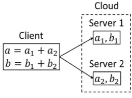
The system used in this paper is composed of a client and mservers. Each data is divided intompieces of numbers and is sent to each server (Fig.1 form= 2). Each server performs its computation and sends the computation result to the client. The client can get the result using them. If the result is not obtained by one processing, then the multiple processing is repeated. As for the cloud system, there are many methods of secure preserving, but it seems that SMC method using distributed processing is suitable for the system. In particular, three types of conventional methods for partitioning data to be securely shared are well known [3], [4]. They are known as horizontal, vertical and arbitrary partitioning methods. In the following, the horizontal method is only explained by using a data example of students’ marks shown in Table I. See Miyajima [8] about the detailed explanation. In Table I, aandb are original data (marks) and ID is the identifier of student. The number of servers is two. The assumed task is to calculate the average of data. The horizontal partitioning method assigns the horizontally partitioned data to servers as follows :

TABLE I

CONCEPT OF HORIZONTALLY AND VERTICALLY PARTITIONED METHODS COMPOSED OF ONE CLIENT AND TWO SERVERS.

Server 2 : data for ID = 3, 4

In the method, Server 1 computes two averages for sub-jects A and B as(22 + 24)/2and(32 + 37)/2, respectively. Likewise, Server 2 computes two averages for subjects A and B as(40 + 13)/2and(40 + 45)/2, respectively. Servers 1 and 2 send calculated averages to the client and the client obtains the averages of subjects A and B as 24.75

and 38.5, respectively. Since each server cannot know half of the dataset, the method preserves privacy (See Table I). Remark that each server also cannot know the result when we consider average values as unknown parameters. The vertical partitioning method is one of processing data for each subject (See Table I). The third method, the arbitrary partitioning method, splits horizontally and vertically the dataset into multiple parts, and the method assigns the split parts to the servers. For any of the above mentioned methods, if the number of servers is fewer, that is, the size of a partitioned data is larger, any server may more easily guess the feature of all the data from its own subset of data. Therefore, the methods need a large number of servers in order to keep privacy and security. On the other hand, the method explained in the next section divides each item of data and seems to keep them even in the case of a small number of servers.

B. Secure divided data for SMC and their application to machine learning

Let us explain secure divided data for the proposed method using Table II [8]. Letaandbbe two marks andm= 2(See Fig.1). Assume that the addition form is used for dividing each item. For example, two marksaandbare divided into two real numbers asa=a1+a2andb=b1+b2as follows: a=a1+a2 :a1= 1(r1/10),a2=a(1−r1/10)

b=b1+b2 : b1=b(r1/10)andb2=b(1−r1/10) wherer1is a real random number for−9≤r1≤9. Ifr1=−1, then a1 = 0.2 and a2 = −2.2 are obtained. Remark that Server 1 and Server 2 have all the data in column-wise of a1 andb1 anda2 and b2 for each ID as shown in Table II, respectively.

Let us explain how to compute the average for subject A using data a. Server 1 and Server 2 compute the average of a1anda2, respectively. In this case, each average in column-wise fora1anda2is1.8and−4.8, respectively. As a result, the average is obtained as−3 from1.8−4.8.

Remark that each data for server is randomized and the method does not need to use complicated computation as the encryption system.

[image:2.595.361.491.58.154.2]

Let us explain about the application of secure divided data to ML. In the conventional methods, the set of learning data

Fig. 1. An example of secure shared data form= 2.

TABLE II

DATA FORSERVER1ANDSERVER2.

Additional form

ID subject A subject B a b

a b r1 a1 a2 b1 b2

1 -2 -6 -1 0.2 -2.2 0.6 -6.6

2 -8 2 -6 4.8 -12.8 -1.2 3.2

3 1 -9 5 0.5 0.5 -4.5 -4.5

Server 1 1.8 -1.7

Server 2 -4.8 -2.6

average -3 -4.3

for ML is shared into some subsets. On the other hand, the proposed one divides each item of the learning data into plural pieces and processes them. From the point of view, SMC algorithms for supervised learning such as BP method and unsupervised learning like k-means method were proposed [8]. Then, how is the algorithm of RL for SMC? In this case, as there do not exist learning data explicitly, the solution is obtained by repeating trial and error. Since there is no data for learning, it seems that the conventional method using subset of learning data is difficult to use. On the other hand, several methods on privacy preserving for RL have been proposed, but these are almost all methods using encryption and homomorphic mapping [13], [14]. The proposed method attempts to realize SMC by simple secret computation processing which does not use such complicated cryptographic processing and homomorphic mapping. That is, the aim to reduce the computational complexity of client while keeping the secret of data (Q-value information in this case). In previous papers, we have already proposed Q-learning and PS methods for SMC in the digital model [9], [10]. In the next section, learning methods using secure divided data in the analog model are proposed.

C. Q-learning methods in the digital and analog models

In the learning, the action is selected based on the Q-value function. If a solution is obtained, Q-Q-values are updated based on the updated formula. By iterating these process, it is known that Q-value function is updated and converges [11]. In the first part of learning, the action for the state is selected randomly and the action becomes decidable as learning steps proceed.

In learning step, Q-value function is updated as

Q(s, a)←Q(s, a) +α△ (1)

△=r+γmax

a′∈AQ(s

′_{, a}′_{)−Q(s, a) (2)}

wherer,αandγ are the reward, learning constant and dis-count rate, respectively. The states′is the next state selected for the statesand the actiona. The termmaxa′_∈AQ(s′, a′) means the Q-value Q(s′, a′₀) for an action a′₀ taking the maximum number of Q(s′, a′). See the Ref. [9] about the example of Q-learning in the digital model.

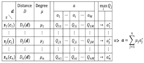
Let us think about the analog model of Q-learning. Let us explain using an example of maze problem to make the story easy to understand. The problem is how the agent can arrive in the shortest path at the goal from the start point (See Fig.2). In the digital model, one of actions at each position is selected. Therefore, the path obtained becomes a zigzag path as behavior. However, in the real problem, it is desirable to get smooth path. An analog model is proposed as a model to realize all directions for behavior (action). Several methods have been proposed for Q-learning for the analog model. Here, we introduce a learning method that determines the action based on the distance between the current position and state (position) of the agent. That is, while hard selection for the action in the digital model is performed, the introduced method achieves a soft matching selection for the action. Let us explain how to select the action of Q-learning in the analog model using Fig.2. Assignnstates (the center positionc) in the space where the agent moves.

Let d be the current position of the agent. First, the distanceDj(d)betweendand the center positioncj of each state for1≤j≤nis computed as follows:

Dj(d) = exp

(

−||d−cj||2

2b2 j

)

(3)

where exp(·)means the Gauss function with the width bj. Remark that Dj(d) is large if the distance between d and

cj is near.

Next, the action a∗_j for each state sj is selected as the action with the maximum number of Q-value (See Fig.2) and the degreeµj of coincide betweend andsj is computed as follows:

µj(d) =∑nDj(d)

i=1Di(d)

for 1≤j≤n (4)

and

n ∑

j=1

µj(d) = 1 (5)

Further, the action a∗ for the agent is determined as the composition of vectors as follow:

a∗=

n ∑

j=1

[image:3.595.303.547.52.159.2]

µja∗j (6)

Fig. 2. The method to determine the action in the analog model.

As a result, the agent at the position d moves in the direction of a∗ and arrives at the new position d′. In this case, the moving distance is selected randomly.

The conventional algorithm for Q-learning is shown as follows :

[Q-learning algorithm for the analog model]

d: the current position.

d0 : the initial position.

Q(s,a): Q-value for the statesand the actiona. S : The set of states.

A: The set of actions.

tmax : The maximum number of learning time. Tmax andTmin: Constants for Boltzmann selection.

cj : The center position of the statesj for 1≤j≤n. Dj(d) : The distance between the statesj and the placed for Eq.3.

ε: The probability forε-greedy selection method.

p : The real number selected randomly from the interval

0≤p≤1. Step 1

Let R+ and R−, α and γ be plus and minus reward, learning constant and discount rate. LetS andAbe defined. Let Q(s,a) = 0 for s∈S and a∈A. Let t = 0. (Let ε be defined forε-greedy selection method.)

Step 2

Letd←d0 be the start position.

Step 3

The distance Dj(d) and the degree µj for 1≤j≤n are computed from Eqs.3 and 4.

Step 4(In the case of Boltzmann selection method) The actiona∗_j at the statesj is selected based on the value B(sj,a)as follows :

B(sj, a) = ∑exp (Q(sj, a)/T)

b_∈Aexp (Q(sj, b)/T)

(7)

T = Tmax× (

Tmin Tmax

) t Tmax

(8)

Leta∗_j be the selected action based on Eqs.7 and 8. That is, the actiona∗_j from the setA is selected with the probabilityB(sj, a).

Step 5

The actiona∗ at the place dis computed using Eq.6. Letd′be the next position determined from the actiona∗. Step 6

Q(sj,a∗_j)←Q(sj,a∗j) +µjα(r+△) (9)

△=

n ∑

j=1

{γµ′_jmax

a′_j∈A

Q(s′_j, a′_j)−µjQ(sj, a∗j)} (10)

, where µ′_j,s′_j anda′_j are parameters for d′ and if d′ is in the goal area, thenr=R+ _{and go to Step 7 else ifd}′ _{is not} in the movable place(state), thenr=R− and go to Step 3 else r= 0and go to Step 3.

Step 7

Ift=tmax then the algorithm terminates else go to Step 3 with t←t+ 1.

If the ε-greedy method is used instead of Boltzmann selection, Step 4 is replaced with the following Step 4’ : Step 4’(In the case of the ε-greedy selection method)

Let p be the real number randomly selected. The action a∗_j for the statesj is selected based onε-greedy selection as follows :

a∗_j =

{

a s.t. maxa∈AQ(sj,a) for p≥ε (a)

randomly selected for otherwise (b) (11)

That is, if pis greater than or equal toε, then the action

a∗_j satisfying the condition of Eq.11(a) is selected otherwise the actiona∗_j is randomly selected.

III. Q-LEARNING FOR SECURE MULTIPARTY COMPUTATION IN THE ANALOG MODEL

In Q-learning for SMC on cloud system, Q-values are divided to each server in addition form . Each server updates divided Q-values and sends the result to the client. The client can get new Q-values by adding the results ofmservers. The process is iterated until the evaluating value for the problem satisfies the final condition. The problem is how Q-values on the client are updated using Q-values divided on each server. The divided representation of Q-value is given as follows :

Q(s, a) =

m ∑

k=1

Qk(s, a)f or s∈S and a∈A (12)

In the following, two learning methods are proposed. The proposed methods can be easily applied to other Q-learning algorithms in the analog model.

A. Q-learning for SMC

The first algorithm using Boltzmann (ε-greedy) selection method is shown in Table III. The initial values of client and servers are set in Initializing Step. In Step 1, the initial position is set. In Step 2, the distanceDj(d)and the degree µi for the current position dand each center positioncj of statesjfor1≤j≤nare computed. In Step 3, the actiona∗jfor the statesjis selected based on Boltzmann selection method. Further, the next actiona∗ is determined as the vector sum of a∗_j for1≤j≤nand the new position d′ is obtained from the action a∗. Furthermore, the degree µj′ of coincide for the positiond′is computed fromd′andsj(1≤j≤n). In Step 4, the updating rate △k_b for b∈A and1≤k≤m is computed

in each server. In Step 5, the updating rate△∗ is computed using △k

b for b∈A and1≤k≤m. Further, the updating rate ξk for each server is determined usingβk(sj,a∗_j)and△∗. It means to divide△∗intompieces of numbers. In Step 6, the Q-valueQk(sj,a∗_j)for each server is updated. In Step 7 and Step 8, it is checked if the final condition satisfied or not. If the final condition is not satisfied, then the next episode is iterated. The algorithm is called M1 method.

B. Q-learning with dummy updating

In M1 method, designated Q-values are updated based on µj for 1≤j≤n. Therefore, there is the possibility that the server knows information on which Q-value is important. In order not to inform the server of the update information, an improved method with dummy updating is proposed in which all the Q-values are updated.

The fundamental idea of Q-learning with dummy updating is that all Q-values are updated at each step. Therefore, it seems that each server cannot know which Q-value is im-portant or not. Let us explain the improved M1 method. The numberpk(s,a)is randomly selected such that|pk(s,a)|≤1 andηk(s,a)is calculated as follows :

ηk(s,a) =

      

pk(s,a)

∑m

l=1pl(s,a)

for s=sj anda=a∗j (A)

for 1≤j≤n pk(s,a)

∑m

l=1pl(s,a)

− 1

m for otherwise (B)

(13)

wheres=sj anda=a∗j for1≤j≤nare selected states and actions.

Remark that each case of A and B for Eq.13 holds ∑m

k=1ηk(s,a) = 1 and 0 for s∈S and a∈A, respectively. That is, all Q-values for states and actions are randomly updated usingpk(s,a)and each server cannot know which Q-value is import or not at each step.

In the improved method, Steps 8 and 9 of Table III are changed as follows :

Step 8 (Client)

Calculate ηk(s,a) of Eq.13 for s∈S and a∈A. Let ξk = αηk(s,a)△∗ for 1≤k≤m. Send ξk for 1≤k≤m to each server.

Step 9 (k-th Server)

The Q-valueQk(sj, ai)is updated as follows :

Qk(sj, ai)←Qk(sj, ai) +µjξk (14)

The algorithm is called M2 method.

IV. NUMERICALSIMULATIONS FOR THE PROPOSED ALGORITHMS

In numerical simulations, the problem is to find the shortest path for the agent from the start position to goal area by Q-learning methods (See Fig.3). In Fig.3, the agent can go to any position except for black and outer areas. In order to find the shortest path, the agent iterates trials to move from the start to goal area based on each algorithm. The simulation conditions are as follows:

1) Let the start position d0 = (1,1), black(wall) area B = {(x1, x2)∈R2|4≤x1, x2≤6} and the goal area

TABLE III

M1METHOD OFQ-LEARNING FORSMC.

Client k-th Server (1≤k≤m)

Initialization The numbersR+_,R−_{,r,αandγare given. Lett= 0. LetQk(s, a) = 0fors∈Sanda∈A.}

Step 1 Letd←d0.

Step 2 CalculateDj(d)andµjfordandcj(1≤j≤n).

Step 3 Send all Q-valuesQk(s,a)fors∈Sanda∈Ato the client. Step 4 CalculateQ(s,a) =∑m

k=1Qk(s,a)fors∈Sanda∈A.

Select the actions∗_jfor the statesjbased on Boltzmann selection of Eq.(7). Leta∗=∑n_j=1µja∗jbe the vector sum ofa∗_j(1≤j≤n). Letd′be the next position determined bya∗. The degreeµ′_jof coincide betweend′andsjfor 1≤j≤nis computed.

Step 5 If the positiond′is possible(movable), then send the degree

µjandµjfor1≤j≤nto each server else go to Step 4.

Step 6 Calculate△k

b=rµ′jQk(s′j, b)−µjQk(sj, a∗j)for1≤j≤n and send them to client.

Step 7 Calculate△b=

∑n k=1△

k

band△∗=r+ maxb∈A△b and sendr+△∗_{to all servers, wherer=R}+_,R−_and

0 ifd′is in goal, not in movable position and otherwise, respectively.

Step 8 Selectmpieces of random numbersβk(s, a) s.t.∑m_k=1βk(s, a) = 1. Letξk=αβk(sj, aj)△∗for 1≤k≤m. Sendξkfor1≤k≤mto each server.

Step 9 The Q-valueQk(sj, a∗j)is updated as follows :

Qk(sj, a∗j)←Qk(sj, a∗j) +µjξk Step 10 Ifd′is in goal state, then go to

Step 11 else go to Step 2 withd←d′. Step 11 Itt=tmaxthen the algorithm terminates

else go to Step 1 witht←t+ 1.

Fig. 3. The figure for the maze problem.

2) Let A = {0,π₂, π,3₂π} and the set of central positions C(S) ={(x1, x2)∈Z2|1≤x1, x2≤9}−B, where each of the setAmeans four directions up, down, right and left on Fig.3, andZ is the set of all integers. Letn=|C(S)|. The states are arranged in a lattice pattern at regular intervals.

3) LetTmax= 5.0 andTmin= 0.03for Boltzman selection andε= 0.1for ε-greedy selection.

4) The moving distance h for the agent at each position

d is selected randomly for 0.01≤h≤0.5 and the action is determined by each algorithm.

5) If the agent selects to move to wall or outer area, the agent ignores the selection and reselects a new action, where r=−1 is given as the negative reward. It is not counted in the number of trials.

6) If the agent arrives at the goal area in the maximum number of learning time, then the agent starts the new trial, where the reward r= 1is given as the positive reward. 7) Lettmax= 10000,r= 10,α= 0.5,γ= 0.92, andm= 3

and10. Twenty trials for learning and test are performed for each algorithm.

8) In the test simulation, experiments are carried out with

five positions as the starting points as shown in Fig.3. The result is evaluated as the rate of the number of success trials and the average of moving distance from each starting point to goal area.

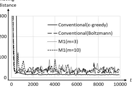
Figs.4 and 5 show the efficiency graphs. They represent the moving distance to the learning time. In Figs.4 and 5, the conventional (ε-greedy or Boltzmann), M1 for m = 3

and10, and, M2 form = 3 and10 mean the conventional algorithm withε-greedy or Boltzmann as selection method, proposed algorithms for M1 with m = 3 and 10, and for M2 with m = 3 and 10, respectively. All the results are almost the same as the conventional cases. Table IV shows the results of the test simulation, where Tests 1 to 5 mean the cases with different starting points as shown in Fig.3. In Table IV, No. Suc. and M.D. mean the number of success trials for twenty trials and the average of moving distance for success trials. Further, the result on each server means one in the cases where the same trials are performed using only Q-values of each server. For example, 0.95 of No.success and 9.83 of M.D. for Test 1 of client in the conventional method mean19/20and 9.83 steps as the average for 20 trials to the goal from the start point of Test 1. All the results for client are almost the same as the conventional. As for servers, trials only using server’s information are almost unsuccessful and a lot of times are needed even in the successful cases.

Finally, let us explain about the result of selection meth-ods. The ε-greedy method is in learning time faster than Boltzmann method. But, Boltzmann method is superior in accuracy of the test simulation toε-greedy method. There-fore, we showed the result of Boltzmann selection method in the result of test simulations.

V. CONCLUSION

TABLE IV

THE RESULT OF OPTIMALITY OFQ-LEARNING.

Test 1 Test 2 Test 3 Test 4 Test 5

No.Suc. M.D. No.Suc. M.D No.Suc. M.D No.Suc. M.D No.Suc. M.D Conventional Client 0.95 9.83 1.0 9.62 1.0 5.71 1.0 11.06 0.95 12.75

(m= 3) Client 1.0 10.75 1.0 9.70 1.0 7.00 1.0 11.20 0.95 11.95

M1 Server 1∼10 0.05 0 0.13 0.10 0.05

(m= 10) Client 0.95 10.31 1.0 10.17 1.0 5.66 1.0 11.24 1.0 11.47

Server 1∼10 0 0 0.05 0 0

(m= 3) Client 0.95 9.75 1.0 9.34 0.95 5.34 1.0 11.23 1.0 18.46

M2 Server 1∼10 0 0 0.05 0.05 0.05

(m= 10) Client 1.0 10.32 1.0 9.83 1.0 5.29 1.0 10.72 1.0 11.46

[image:6.595.67.527.85.191.2]

Server 1∼10 0 0.05 0.025 0.05 0.05

Fig. 4. The result of efficiency of Q-learning for SMC.

Fig. 5. The result of efficiency of Q-learning for SMC.

shown in numerical simulations. In Section 2, cloud com-puting system, related works on SMC and a secure data dividing mechanism used in this paper were explained. Further, Q-learning methods in the digital and analog models are introduced. In Section 3, Q-learning methods in the analog model for SMC were proposed. First, a Q-learning algorithm in the analog model was proposed using divided Q-values and the effectiveness was shown. The feature of Q-learning method for the analog model was that the action was selected as the weighted sum of plural actions. In the proposed algorithm, there was the possibility that some

servers know secure computation. Therefore, an improved Q-learning algorithm in the analog model was proposed. It was the method with dummy updating and it seems that any server is difficult to know secure computation. In section 4, numerical simulations for a maze problem were performed to show the performance of proposed methods. In the future, we will reduce the computational complexity of the client and show the safety of algorithms for SMC in theoretical proof.

REFERENCES

[1] A. Shamir, ”How to share a secret”, Comm. ACM, Vol. 22, No. 11, pp. 612-613, 1979.

[2] S. Subashini, and V. Kavitha, ”A survey on security issues in service delivery models of cloud computing”, J. Network and Computer Applications, Vol.34,pp.1-11, 2011.

[3] A. Ben-David, N. Nisan, B. Pinkas, ”Fair play MP: a system for secure multi-party computation”, Proceedings of the 15th ACM conference on Computer and communications security, pp.257-266, 2008. [4] R. Cramer, I. Damgard, U. Maurer, ”General secure multi-party

computation from any linear secret-sharing scheme”, EUROCRYPT 2000, pp.316-334, 2000.

[5] J. Yuan, S. Yu, ”Privacy Preserving Back-Propagation Neural Network Learning Made Practical with Cloud Computing”, IEEE Trans. on Parallel and Distributed Systems, Vol.25, Issue 1, pp.212-221, 2013. [6] N. Rajesh, K. Sujatha, A. A. Lawrence, ”Survey on Privacy Preserving

Data Mining Techniques using Recent Algorithms”, International Journal of Computer Applications Vol.133, No.7, pp.30-33, 2016. [7] K. Chida, et al., ”A Lightweight Three-Party Secure Function

Evalu-ation with Error Detection and Its Experimental Result”, IPSJ Journal Vol. 52 No. 9, pp. 2674-2685, Sep. 2011 (in Japanese).

[8] H. Miyajima, N. Shigei, H. Miyajima, Y. Miyanishi, S. Kitagami, N. Shiratori, ”New Privacy Preserving Back Propagation Learning for Secure Multiparty Computation”, IAENG International Journal of Computer Science, Vol.43, No.3, pp.270-276, 2016.

[9] H. Miyajima, N. Shigei, S. Makino, H. Miyajima, Y. Miyanishi, S. Kitagami, N. Shiratori, ”A proposal of privacy preserving re-inforcement learning for secure multiparty computation”, Artificial Intelligence Research, Vol.6, No.2, pp.57-68, 2017.

[10] H. Miyajima, N. Shigei, H. Miyajima, N. Shiratori, ”A proposal of profit sharing method for secure multiparty computation”, International Conference on Innovative Computing, Information and Control, 2017 (in print).

[11] C. J. C. H. Watkins, P. Dayan, ”Q-learning”, Machine Learning 8, pp.55-68, 1992.

[12] R. S. Sutton, A. G. Barto, ”Reinforcement Learning”, MIT Press, 1998. [13] C. Gentry, ”Fully homomorphic encryption using ideal lattices”, STOC

2009, pp.169-178, 2009.

[image:6.595.57.287.226.383.2]