Parsimonious modeling of inelastic systems

(1)

Thesis by

Dar-Yun Chiang

In

Partial Fulfillment

of the Requirements

for

the Degree

of

Doctor of Philosophy

California Institute of Technology

Pasadena,

California

1993

(2)

(3)

ACKNOWLEDGEMENTS

I am heartily grateful to my advisor, Professor James L. Beck, for his continued guidance and encouragement throughout the course of my study and research at Caltech. His infectious enthusiasm and continuous availability to advise me with my work are greatly appreciated.

I would like to thank the California Institute of Technology for the generous financial support offered to me, which made my study here possible. I also wish to express my gratitude to the people in Thomas Lab, who created a friendly environment making my stay here a very enjoyable experience. My special thanks are extended to Dr. Jay C. Chen, who was at JPL and is now in the Hong-Kong University of Science and Technology, for his constant help that made my overseas study here so pleasant and memorable.

(4)

ABSTRACT

Analytical modeling of one-dimensional hysteresis and general multi-axial cyclic plasticity is studied, with particular emphasis on the parsimony of model parameters and the physical consistency of model behavior. General criteria for good models are proposed to provide guidelines to the modeling studies conducted in this research.

Various one-dimensional hysteretic models are examined in detail, including both deteriorating and non-deteriorating models. A general formulation for modeling of degrading systems is presented based on the formulation of the Distributed-Element Model (DEM) and the introduction of a damage index function. A new class of deteriorating Masing models, whose behavior can be completely described by a few simple mathematical rules and the extended Masing rules, is also developed to sub-stitute for a special class of deteriorating DEMs, so that their applicabilty to system identification studies is improved.

(5)

LIST OF TABLES AND FIGURES

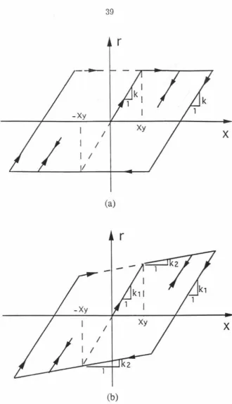
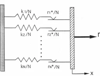
Figure 2.1: Comparison of response histories obtained using the fast algorithm and the 4-th order Runge-Kutta method ... 14 Figure 3.1: Hysteretic restoring force behavior of (a) the elasto-perfectly plastic model (b) the bilinear model . . . 39 Figure 3.2: Response behavior of the Bouc-Wen model (a) restoring force diagram

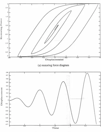
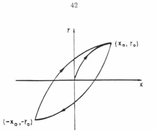
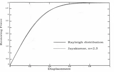
(b) prescribed displacement history . . . 40 Figure 3.3: The unstable drift exhibited by the Bouc-Wen model . . . 41 Figure 3.4: The Distributed-Element Model for one-dimensional hysteresis ... 41 Figure 3.5: Masing's hypothesis for cyclic hysteretic loops . . . 42 Figure 3.6: Hysteretic loops for transient loading ... . 42 Figure 3.7: Effect of the parameter n of a special class of Masing models [24] on the

smoothness of yielding curves . . . 43

Figure 3.8: Effects of the degrading parameters on the behavior of the deteriorating Bouc-Wen model (from [52]) . . . 44 Figure 3.9: Restoring force diagram of a typical breaking element in the

maximum-displacement-controlled deteriorating DEM ... 45 Figure 3.10: Restoring force behavior of the maximum-displacement-controlled

deteriorating DEM subject to an earthquake excitation (from [22]) 45 Figure 3.11: Simulated restoring force behavior of the proposed deteriorating Masing

model ... 46 Figure 3.12: Comparison of the behavior of two matching Masing models ... 47 Figure 3.13: Distribution curves described by the generalized Rayleigh distribution

function with different values of n ... 47 Figure 3.14: Plastic deformation of the Masing model based on a statistical

interpreta-tion of the Rayleigh yield-strength distribution function ... 48 Figure 3.15: Drift response of a Masing model based on the Rayleigh distribution

(8)

Figure 3.16: Different types of elements used in a model for hysteretic systems with stiffness degradation (from [13]) ... 49 Figure 3.17: Configuration and behavior of Gates' degrading model (from [13]) . 50 Figure 3.18: Clough's hysteretic model for stiffness-degrading behavior ... ... 51 Figure 3.19: Takeda's hysteretic model for reinforced concrete structural systems 51 Figure 3.20: Saiidi & Sozen's hysteretic model for stiffness-degrading behavior .. 52 Figure 4.1: Behavior of the endochronic model using the kernel function defined by

Eqn. (4.18) ... 69 Figure 4.2: A typical yielding curve for illustration of the proposed modeling technique based on the endochronic theory . . . 69 Figure 4.3: Effect of the parameter p of the proposed class of endochronic models on

the yielding behavior . . . 70 Figure 4.4: Response behavior of a one-dimensional endochronic model and a

match-ing Masmatch-ing model . . . 70 Figure 4.5: Uniaxial cyclic hardening behavior of (a) a Masing model (b) a real

material . . . 71 Figure 5.1: Two different one-dimensional Distributed-Element Models (a)

parallel-series model (b) series-parallel model ... 109 Figure 5.2: Illustration of the space-dependent yielding behavior of ideal plasticity 110 Figure 5.3: Invariant yield surfaces nested in the element stress space ... 111 Figure 5.4: Selection of yield constants for a finite number of elements according to

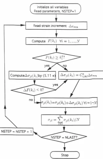
a specified yield-strength distribution function ... 111 Figure 5.5: A flow diagram showing numerical procedure for obtaining stress response

of anN-element DEM ... 112 Figure 5.6: Prescribed strain loading paths for response studies of the proposed

(9)

Figure 5.8: Experimentally-observed stress response of copper to the prescribed strain path given in Figure 5.6(b) ... 115 Figure 5.9: Stress response predicted by a new DEM subject to the prescribed strain

path given in Figure 5.6(a) ... 116 Figure 5.10: Stress response predicted by a new DEM subject to the prescribed strain

path given in Figure 5.6(b) ... 117 Figure 5.11: Response predicted by different plasticity models to the strain path given in Figure 5.6(b): (a) von Mises' yield surface with Prager's hardening rule (b) Tresca's yield surface with Ziegler's hardening rule (c) Tresca's yield surface and limit surface with Mroz' hardening rule ... 118 Figure 5.12: Response behavior of ideal plasticity under a proportional strain loading

path (a) proportional strain path (b) stress response behavior .... 119 Figure 5.13: Definition of the plastic-relaxation stress increment in the uniaxial case ... 120 Figure 5.14: Illustration of the existence of equilibrium points associated with a big

strain cycle (a) a strain cycle (b) the corresponding stress response 121 Figure 5.15: A diagram showing the rotation of coordinate axes which makes the x1 axis perpendicular to the tangent plane to the yield surface 80.0 at Qo ... 122 Figure 5.16: An illustrative diagram showing non-strict convexity of yield surfaces 122

Figure 6.1: Hysteretic behavior of the two-dimensional Bouc-Wen model (a) propor-tional displacement path (b) hysteretic restoring force behavior . . . . 142 Figure 6.2: Comparison of the initial response predicted by Eqn. (6.16) and by aDEM ... 143 Figure 6.3: The Mroz kinematic hardening rule for multiple yield surfaces ... 144 Figure 6.4: A biaxial strain path for the study of the proposed response formulas for

initial loading ... 144 Figure 6.5: Experimentally-observed stress response of copper to the strain path given

(10)

given in Figure 6.4 • • • 0 0 • • • • • 0 0 0 0 0 • • • • 0 • • 0 • • 0 0 0 • • 0 0 • • 0 0 0 0 • • •• • • 0 • • • 146

Figure 6.7: Stress response predicted by Eqn.(6.13) with the prescribed strain path

given in Figure 6.4 ... ... 147

Figure 6.8: Movement of yield surfaces with current stress state moving from A to B

(a) initial configuration (b) current stress state A (c) current stress state B ...... 148

Figure 6.9: Different yield surfaces and shifted 1r planes in the principal stress space

(a) von Mises yield surface (b) Drucker-Prager yield surface ... 149

Figure 6.10: A schematic diagram showing transformation on the 1r plane ... 150

Figure 6.11: Illustration of completed loops and numerical difficulty associated with the transformation approach ... 151

Figure 6.12: Geometrical considerations of transient response (a) unloading from

point A (b) unloading from point B with new center C . . . 152

Figure 6.13: Stress response predicted by a generalized Masing model subject to the strain path given in Figure 5.6(a) ... 153

Figure 6.14: Stress response predicted by a generalized Masing model subject to the

strain path given in Figure 5.6(b) ... 154

Figure B.1: Geometrical configurations before and after transformation ... 169

Figure B.2: Configurations at different transformation stages ... 170

(11)

CHAPTER 1

INTRODUCTION

Most structures exhibit nearly linearly elastic restoring force behavior under moderately small loading conditions. However, when subjected to severe excitations such as strong earthquake ground motions, structures may respond inelastically and exhibit hysteretic behavior so that the restoring force at a time instant depends not only on the instantaneous state, but also on the past response history. The study of nonlinear, hysteretic behavior of mechanical systems has been of great interest to researchers in many engineering fields, and particularly in earthquake engineering [4, 9, 10, 13, 18-24].

Structures of simple configurations and homogeneous materials may usually be approximated by simplifed analytical models so that their response to complicated external loading can be analyzed more efficiently. For example, normal building structures under seismic excitations can often be modeled as shear buildings (i.e., chain models) so that their response characteristics, such as natural frequencies, maximum displacement response, etc., can be estimated efficiently and with rea-sonable accuracy. When such simplified models are used, the hysteretic response of structural systems is often described by its overall interstory force-deflection re-lationship so as to avoid complex stress-strain calculations for which constitutive equations governing material behavior at a point are needed [23].

Although overall planar force-deflection representations in nonlinear structural

(12)

As mentioned earlier, linear models for mechanical systems are, in general,

sufficient to represent system response resulting from small excitations. The

mathe-matical representations of such linear models are usually simple and of clear physical

significance. Thus, modeling of linear systems may be thought of as an easy and

straightforward task, if considered solely from the viewpoint of forward analysis. If

system identification is under consideration, however, the choice of a suitable class

of linear models may become crucial to the success of the model identification from

response data. For example, if linear models are to be used in the identification

of structures using earthquake data, one should consider identifiable modal models

with parameters of modal frequencies, dampings, and mode shape components, not

the models in the physical coordinates with parameters of stiffness and damping

matrices, as recommended by Beck (3], so that more reliable results can be obtained in the case of a limited number of measurement channels. Once the modal

parame-ters are estimated from the earthquake data, they can be used in a subsequent stage

to investigate the generally nonunique inverse problem of going from the incomplete

set of modal parameters to structural stiffness parameters.

In contrast to linear models, nonlinear models are usually more

mathemati-cally involved, especially when hysteretic behavior is taken into account. For the

simplified force-deflection relationship which is a one-dimensional formulation of sys

-tem behavior, numerous models have been proposed ranging from simple ones such

as elasto-perfectly-plastic and bilinear hysteretic models to sophisticated ones like

Takeda's and the Bouc-Wen's models [44, 51]. Among these models, the

Distributed-Element Model (DEM), developed by lwan [19], has been successfully applied to

structural dynamic analysis because ofits physically consistent behavior. The DEM

consists of an assemblage of simple ideal elasto-plastic elements that have different

yield strengths governed by some distribution function. As shown by Jayakumar

[23], the DEM formulation is mathematically equivalent to a general class of Masing

models in which Masing's hypothesis is extended for transient behavior of general

hysteretic response.

An interesting problem that has not been resolved so far is how the Masing

rules can in some way be extended to two or higher dimensions, and how would

(13)

if available. Furthermore, how would the behavior of such general models compare

with those based on the classical theory of plasticity? If these questions can be

answered clearly, then modeling of general plastic behavior of mechanical systems

can be improved and analysis of complex structures can be performed with more

success than before.

We remark that not all modeling of structural systems can be done based

exclu-sively on theoretical considerations. In most cases, the mathematical models are so

complicated that an empirical approach is needed to identify an appropriate model

from within a prescribed class of models using structural response data. Therefore,

it is of practical importance to build new models also from the system identification

point of view. In general, a good model should be not only mathematically simple,

physically consistent, and computationally efficient, but also parsimonious in the

number of parameters.

This thesis consists of five independent, yet interrelated chapters in addition to

Chapter 1, the introduction, and Chapter 7 in which summary and conclusions of

this research are given. In Chapter 2, important issues and practical considerations

of system identification are discussed with particular emphasis on the process of

model building. Criteria of good models for mechanical systems are also proposed

based on considerations of system identification, which provide useful guidelines for

the modeling studies conducted in this research.

Chapter 3 gives an extensive review and discussion of various models for

mod-eling of one-dimensional hysteretic behavior, including both the models defined by

empirical rules and those by differential equations. In particular, the DEM and

Masing models are described in detail, since they form the fundamental starting

points of the present research. Hysteretic models including strength and/ or

stiff-ness deterioration are also discussed in this chapter. An extension of the hysteretic

response rules based on Masing's hypothesis to the case where degradation effects

are included is proposed using the distributed-element formulation and the

intro-duction of a "damage" function. Explicit mathematical rules are then derived for

a particular class of maximum-displacement-controlled deteriorating DEMs [22].

(14)

DEMs becomes simpler as compared with the direct computation of model response by keeping track of response behavior of all the elements constituting the model. As a result, identification studies based on such models can then be performed with more efficiency and higher accuracy. Response behavior of this new class of degrad-ing Masing models is compared with those of other well-behaved degrading models. Of particular interest is the response behavior of a class of endochronic models that are described theoretically by integra-differential equations [46, 47]. The flexible, physically consistent behavior of the modified one-dimensional endochronic model motivated the study of the general endochronic models for cyclic plasticity in which complicated multi-axial loading conditions are considered. This is presented in Chapter 4.

Although the behavior of the modified endochronic models is govened by some mathematically involved integra-differential equations, effective procedures for con

-stitutive modeling based on the theory have been established in the past so that numerical implemention of the models is practically feasible. A new way of modeling based on the endochronic theory is proposed in Chapter 4, which was inspired by the modeling technique used in the Masing models. With the introduction of this new modeling technique, the building process of endochronic models is much simpler and identification studies of systems modeled by endochronic theory then become easier in practice. Furthermore, inspired by the study of the endochronic theory for cyclic hardening behavior, the one-dimensional Masing models (or D EMs) are extended, in a very effective way, to account for cyclic hardening behavior.

In Chapter 5, the one-dimensional DEMs are generalized to three dimensions ( multi-axialloading case), so that they can be used for constitutive modeling of com

(15)

and the associated numerical scheme for implementing the solution algorithm is ef -ficient

as

well. The new DEM is shown to not only provide more accurate response predictions for experimental results compared with models based on the classical theory of plasticity, but it also serves

as

a good physical model through which response mechanisms of complicated plastic behavior can be clearly pictured and elucidated. A rather complete mathematical work regarding the properties of the new DEM, such

as

the existence of equilibrium points and that of a limit surface, will also be covered in Chapter 5.

Though the general multi-dimensional DEM provides a useful and efficient way of constitutive modeling for cyclic plasticity, to implement the theory only a limited number of elements can be introduced due to practical concerns. An interesting question then remaining is whether some mathematical rules can be found which are similar to those used in the one-dimensional Masing models so that even in the general multi-axial loading case, model response can be found without the need of keeping track of each element's behavior. This problem is solved with success in Chapter 6. By introducing a formula good for initial response under multi-axial loading, further unloading and reloading response can then be found by applying a composition of proper transformations to the state variables involved in the formula. This method is theoretically equivalent to that utilizing the classical multi-yield-surface theory with the Mroz kinematic hardening rule [35]. However, it's only with this new approach proposed here that the response behavior of a model with an infinite collection of yield surfaces can be analyzed. Computational efficiency is also preserved in the algorithmic implementation of this new theory, whose validity is confirmed by modeling some biaxial tension-torsion tests [17, 30) under non -proportional cyclic loading conditions. A comparison between the models based on the new approach and the multi-dimensional DEMs is also made at the end of Chapter 6.

(16)

CHAPTER 2

SYSTEM IDENTIFICATION AND MODELING

2.1 Introduction

Engineering problems may usually be classified as direct (forward) or inverse

according to the nature and purpose of the analysis. Direct problems are those of finding the response of systems to specified input excitations; whereas in inverse

problems, the output response to some input is known but either the physical process

(the system) or the input excitation is unknown. System identification may be

de-fined as the process of systematically determining a model of a physical system from its observed input and output data , and so it falls obviously into the category of inverse problems. In general, system identification problems can be further divided into two categories: nonparametric identification and parametric identification. If

the detailed mathematical description of a system is totally unknown or of little inter-est, then we have a nonparametric identification problem or a so-called "black box"

identification problem, in which a functional relationship between input and output is to be determined. On the other hand, if some knowledge of the mathematical

structure of the system is available and the problem is that of determining unknown parameters within the structure, then it is a parametric identification problem. In

engineering applications, the main interest is usually in parametric identification problems in which an optimal model out of a certain class of models is to be found for the system under consideration so that prediction of future performance of the

system can be improved accordingly. In a parametric identification problem, the

in-troduction of model structure usually reduces statistical variability of the estimated

model. Also, the identification problem actually becomes a parameter estimation

problem since the mathematical structure of the model is already specified.

In the following sections, practical considerations about system identification

(17)

2.2 Practical Considerations of System Identification

Identification of structural systems through the use of experimental data is of

considerable importance in many areas of engineering studies, particularly in the fields of structural vibration and system control. Identification problems usually are

considerably more difficult than forward (response analysis) problems due to the

following reasons:

1) The requirement of well-posed analytical models is more critical to identification

problems than to forward problems.

2) A characteristic feature of identification problems is that the accuracy of

iden-tification results is degraded by a combination of measurement, modeling, and numerical errors.

3) The problem of existence and uniqueness of solution (i.e., identifiability

prob-lem) is usually very difficult to be resolved due to practical limitations.

The main purpose of a system identification study is to appropriately represent

the physical structure of a system for response prediction, not just to accurately

reproduce the observed data. To this end, the parametric identification approach

is usually adopted in engineering applications due to its capability of making fur

-ther predictions. Three important stages are included in a parametric identification

problem. The first one is model selection, i.e., choosing a mathematical

formula-tion to represent the physical structure of a system. The second stage is parameter

estimation, which is the determination of the "best" parameters for the specified

mathematical structure for the system. The final stage is model validation, in which

some tests on the identified model are conducted to see if the model adequately

represents the system with respect to the desired objectives. Though the nature of

the three stages are quite different, they are all important to the success of

identi-fication studies. Generally speaking, model selection deals with the application of appropriate physical laws to the systems under consideration. From these laws, some

relations involving parameter variables follow, such as equations for constitutive laws in modeling of stress-strain relationships of materials. In a parametric identification

(18)

of models. Thus far, many systematic approaches have been developed for finding

optimal parameters within a class of models. These identification methods almost

always involve minimization of some error criterion functions. Three widely-used

approaches based on different error criteria are as follows:

1) Equation-error method : The discrepancy between the model equation and the

measured I/0 data is minimized through a regression analysis technique. This

method is simple and computationally effective. However, complete

measure-ments of all the state variables involved in the model equation are required for

the method to be effective, which is usually a severe restriction in practical

problems.

2) Output-error method: The difference between the output of a system and that

of the model in response to some input is minimized by some functional min

-imization technique. This is probably the most widely-used approach in

prac-tical system identification problems due to its great flexibility and moderate

mathematical tractability.

3) Combined method: One can take a combined equation-error/output-error

ap-proach to perform the identification analysis, such as the Kalman filter method

[25, 28] developed for optimal sequential estimates of parameters and states of

a system. These kinds of sequential estimation methods are good for modern

control problems which require real-time (on-line) analysis capability.

An important aspect of the different identification approaches is that they can

be formulated within a unifying statistical framework [6]. For example, the estimate

obtained from the classical output-error least-square method used extensively in

earthquake engineering can be shown to be equivalent to the classical

maximum-likelihood estimate [33], and to that based on Bayesian statistical inference [7],

under the assumption that the output error can be modeled as a Gaussian white

process.

Probably, the most difficult and important issue of parametric identification is

the problem of identifiability of parameters, which refers to the capability of uniquely

determining the parameters of a model from the available I/0 data. The problem of

identifiability can exist even in some of the simplest cases of identification due to the

(19)

estimated from seismic excitation and response histories, the stiffness and damping

matrices of the system may not be determined uniquely in typical situations, as

pointed out by Beck [3]. Instead, modal models consisting of dominant modes in

the response should be used for the identification purpose, and if estimation of

system parameters in the physical coordinates is of interest, a further analysis can

always be done in a separate stage utilizing the original data as well as the modal

data already obtained.

Recently, Beck and Katafygiotis [7] addressed the issues of model identifiability

versus system identifiability of optimal parameters from a class of models. For a set of

parameters to be "model identifiable" (globally or locally), there must exist at most

a finite number of sets of parameter values which give "output-equivalent" models

under a specified input. In contrast, the parameters that are "system identifiable"

determine a finite set of optimal models in which the parameters take the most

probable values out of a class of models given a set of I/0 data. The problem

associated with system identifiability is obviously much more difficult than that of

model identifiability due to the additional considerations of modeling error involved

in the approximate analytical model and measurement noise contaminated in the

response data.

In this thesis work, we are mainly concerned with modeling of general

non-linear mechanical systems. Although there will be no original theory regarding

system identification techniques proposed herein, some new modeling theories to be

presented later are based on practical considerations of system identification. More

-over, the system identification approach is usually the best way to perform model

validation. For this purpose, one could use a set of test data to identify an optimal

model out of the class of proposed models, and then make predictions of response

behavior observed in another experiment using the identified optimal model. In the

next section, some criteria for good analytical models are proposed and discussed

mainly from the identification point of view.

2.3 Criteria for Good Modeling

In engineering problems, direct or inverse, a good model is always of crucial

(20)

depend significantly on the nature of the systems under consideration and may vary

considerably from case to case, there are some general rules that may be consid-ered as modeling criteria for most practical mechanical problems. The criteria are

proposed as follows:

1) Mathematical Simplicity

A model is a mathematical realization of a physical system which may, in

gen-eral, have rather complicated behavior. However, considering practical issues such

as mathematical tractability, a good model should always be as simple as possible

so that it can have greater applicability to widely-spread engineering problems. For

example, in system identification problems, parsimony in parameters of a model not

only makes numerical computation more easy, but also reduces possible

identifiabil-ity problems.

2) Physical Reality:

A good model should be able to capture most of the important features observed

in the physical system to be modeled. Exhibition of abnormal, nonphysical

charac-teristics can sometimes lead to numerical instability even when the model is used

for numerical solution of well-posed physical problems [40]. Following this criterion,

parameters selected in a good model should all have clear physical significances.

3) Modeling Versatility:

A class of models should be able, or can be easily extended, to account for

various effects exhibited by the physical systems of interest. A versatile

mathe-matical model may also possibly serve different purposes in different engineering

applications.

4) Computational Efficiency :

Practical implementation of a good model should be reasonably simple and

computationally efficient so that applicability of such a model will not be limited

by practical concerns. Computational efficiency for numerical implementation of a model is of particular importance from the identification points of view, since

identi-fication processes usually require a large amount of iterations of response calculation.

(21)

The sensitivity coefficients* of the parameters involved in a model should be neither too high nor too low under practical considerations. This property is referred to as robustness of a model. If the sensitivity of some parameters is too high, the

result of a forward response analysis may be significantly degraded by model error;

on the other hand, if it is too low, nonunique result of identification may be obtained. It should be mentioned that in practice it may be difficult to find a model that meets all the criteria listed above. For example, the widely-used Bouc-Wen model [51, 52], which is described solely by a differential equation, can be viewed as both efficient and versatile since it can model various characteristics of hysteresis, and can be easily extended to include the effects of strength and/or stiffness deterioration.

Furthermore, the model is applicable to response analysis, including random

vibra-tion problems, as well as system identification studies [16, 42). However, this model

may not be simple and realistic enough from some practical points of view. For

example, the model may be, in some case, overparameterized such that appropriate choice of the parameter values and identifiability problems can be very tough, as will be discussed later in the chapters that follow. Nevertheless, if a model is always

built with the aformentioned criteria in mind, then reliable behavior and practical

applicability of the model can always be expected.

2.3.1 An Illustrative Example of Proper Modeling

To make the above ideas clearer, in the following we pose an example to show

that a simple, efficient model for forward analysis may lack robustness for

identifi-cation.

Accurate and efficient algorithms have been developed [5] for computing the

re-sponse of a single-degree-of-freedom linear oscillator subjected to an arbitrary forcing

function, in which any desired response quantity can be computed through the use

of a discrete recursive formula based on Duhamel's integral and linear interpolation

* The sensitivity coefficient of a parameter is defined as the change of some

(22)

for the excitation between discrete points sampled uniformly in time. For example,

if acceleration response i(t) of a linear oscillator described by

i

+

2~w

0

x

+

w3x = r(t) (2.1)

is of interest, where ~ and w₀are damping ratio and natural frequency of the system,

one can use the following recursive formula:

(2.2)

(2.3)

to compute the acceleration time history, where subscript i denotes the

timet= ti,

and the expressions for the coefficients can be found in [5). In particular, the two

coefficients b1 and b2 are selected such that the transient response due to initial

conditions is determined exactly. This yields

(2.4)

where no= woflt and Dd = ) 1 - eno. Another interpretation of this choice of b1

and b2 is that it ensures that the poles of the transfer function of the oscillator are

also poles of the transfer function of the algorithm [5). It may be noted that this

model based on the algorithm given by Eqns. (2.2), (2.3) is highly computationally

efficient and, in addition, it gives very accurate results. A comparison of a response

history obtained using the fast algorithm and that using the 4-th order Runge-Kutta

method is shown in Fig. 2.1 for a system with w0 =2Hz and~= 5% subjected to a

scaled El Centro ground motion. The superiority of this algorithm over the

Runge-Kutta method is also prominent in other case studies. Suppose now that this model

is used for an identification study in which the input/ output data, i(t) and r(t),

are given, and the system characteristics ~ and w0 are to be identified. According

to Eqn. (2.2), the coefficients b1, b2 , and c1 can be found easily using regression

analysis technique such as the least-square method. Thus, based on Eqn. (2.4) we

can solve for~ and w0 from b1 and b2 as follows :

(23)

where

(2.6)

This method of identification is also computationally efficient, since there is no

nonlinear optimization process involved in the parameter identification procedure.

However, the identification results using the model based on the foregoing discrete

recursive algorithm will be significantly degraded when there is some noise present.

This is due to a numerical ill-conditioning inherent with the model. It follows from

Eqn. (2.4) that for lightly damped systems, the two coefficients satisfies

(2.7)

1.e., b1 is close to but less than 2, and b2 is close to but greater than -1. If the

identified b1 and b2 satisfy the relations given in (2.7), then the system parameters

~ and

wo

can have reasonable values. However, due to the presence of measurement

noise or numerical error, it is very possible that the values of b1 and b2 identified

using the least-square method do not meet (2. 7). As a result of this, the parameters

~ and

wo

computed using (2.5), (2.6) may become totally unrealistic due to the

logrithmic function involved in Eqn. (2.6). For example, if we have b1 = 2.000,

b2

=

-1.001 and 6.t

=

0.01 sec, then by Eqns. (2.5), (2.6) we find~ ~ 1% and

wo

~ -0.42 Hz, where the negative frequency does not make any sense in reality.

Besides, since ~ and 6.t are usually small in practical dynamic analyses, the error

of

wo

computed using Eqn. (2.5) may become quite large even if the error of the

identified a1 is small.

Through the above example we realize that a model which is simple and

compu-tationally efficient may lack robustness for identification due to the high sensitivity of its parameter values to "noise." However, we remark that if the output-error

method, instead of the equation-error method, is used with the discrete recursive

model, i.e., the optimal parameters ~ and w0 are obtained directly by

minimiz-ing some error function associated with output variables without first finding the coefficients b₁ and b2 , then the lack of robustness of the model vanishes and as

demonstrated by Beck [3], the model actually works well in the modal identification

(24)

5

8

0 0

0.4

0

.

35 ₀.3

1

0

.

25- ₀.2

L 0.15 ~ 0 . 1 0 . 05

,.

,J

I

\

A

'

·

l\

I

\

I

\

/\

j.h\ i

~ p. til _....

-0 . 03 Q -0 . 1 -O . U · 0 . 2

-0.25 -0

. 3 IJ -0 . 33

"''' i.i

(25)

CHAPTER 3

MODELING OF ONE-DIMENSIONAL HYSTERETIC SYSTEMS

3.1 Introduction

Linear models, though mathematically simple, are only good for representing

structure response resulting from small loadings. When subjected to severe

excita-tions such as strong seismic ground moexcita-tions, structures usually respond inelastically

so that nonlinear analytical models are required to adequately represent the

struc-tural behavior. In most cases, the response of a system that is stressed beyond

its "yield point)) into the nonlinear regime depends not only on the instantaneous

state, but also on its past history. The history-dependence phenomenon is generally

referred to as hysteresis. The study of analytical modeling of nonlinear, hysteretic

behavior of mechanical systems has thus been a research area of great interest.

In this chapter, we are concerned with one-dimensional hysteretic models that

can be used to describe nonlinear restoring force-deflection behavior or uniaxial

stress-strain relations of structural systems. The more general modeling of

con-stitutive laws of materials will be discussed later on in the following chapters.

The simplest hysteretic models are probably the elasto-perfectly-plastic model and

the bilinear model, as sketched in Fig. 3.l(a) and (b), respectively. These models

have been used extensively in many engineering applications due to their analytical

tractability. However, they are often too simple to yield good approximation to

real systems. Previous studies [23, 51] indicated that the deviation from linearity

around the yield point of a structural system should have a smooth transition in

general as it reflects the effect of the yielding in an assemblage of many structural

members. Furthermore, these simple models do not account for the hysteretic

en-ergy dissipation at small-amplitude cyclic response after the occurrence of yielding,

which can lead to a higher predicted response level than the actual response [39]. Various mathematical models have been proposed for modeling of hysteretic

behavior of structural systems. A thorough understanding of these models helps

fur-ther modeling processes involved in building up new more general models. However,

(26)

since many good references on this topic are readily available, for example, [23,

45]. Instead, we will concentrate on those models that can give smooth transition

from linear into the nonlinear regime. These models include those described solely

by differential equations involving "hidden variables", physically-based D

istributed-Element Models [19, 20], and the Masing models which are formulated based on

Masing's hypothesis and some extended rules [23].

Since the inelastic response of a structural system is usually accompanied by

stiffness and/ or strength deterioration, it is important to extend the hysteretic

mod-els to account for these effects so that they can be used for modeling of degrading

systems. This will also be investigated in this chapter. A new class of

deteri-orating Masing models will be proposed for identification purposes to substitute

for a class of maximum-displacement-controlled deteriorating Distributed-Element

Models proposed by Iwan and Cifuentes [22].

3.2 Modeling of Hysteretic Systems without Deterioration

3.2.1 Hysteretic Models Described Solely by Differential Equations

Analytical hysteretic models that are described solely by differential equations

in general have the advantage of good mathematical tractability. A well-known

model in this category is the Bouc-Wen model which was originally proposed by

Bouc and later generalized by Wen [51], who also applied this model to random

response analysis of structural systems [52]. The model is completely described by

the following first-order, nonlinear ordinary differential equation:

(3.1)

where r is the hysteretic restoring force and x is the displacement of a system.

The parameters A, a, {3, and n control the slope, amplitude, and shape of the

hysteretic loops and the smoothness of yielding. This model can be shown to exhibit

an exponential type of curvilinear behavior. A simulated response of the Bouc

-Wen model is shown in Fig. 3.2(a), where the model is subjected to a prescribed

(27)

Bouc-Wen model is actually a rate-independent model as Eqn. (3.1) can be put into the form

~:

= A

±

(a

±

,B)

Tn, (3.2)

depending on the signs of

x

and T.

Some special cases of the Bouc-Wen model are noteworthy, as they form the

basis of later investigations on constitutive modeling for the general multi-axial

loading cases. One is the Ozdemir's model without "back-stress"

[36)

which can be

described by the differential equation:

r

x

I

x

I

(

T

)n

To

=

xo -

xo

To

'

(3.3)

where

To

is the yielding force and

x

0 the yielding displacement of a system. Another

way to write Eqn. (3.3) is

(3

.

4)

Note that

To/xo

represents the linear (small-amplitude) stiffness of the system.

Another special case of Eqn. (3.1) can be found by putting A= E, a= 1/Z,

,B

= 0

and n = 1 to yield

1

r

=Ex-

zlxiT,

(3.5)

or

1

dT

=

Edx- z

l

dx

i

T.

(3.6)

Equation (3.6) describes a simple endochronic model*

[46, 47)

as shown by Bazant

and Bhat

[2).

The merit of these models described by differential equations lies in

that they are completely defined by a single differential equation so that their

ap-plications to various engineering problems can be made more easily. For instance, it

is possible to find the closed-form solution of the stochastic equivalent linearization

coefficients for the Bouc-Wen model given by Eqn. (3.1) under some mild

assump-tions of a joint Gaussian distribution on the variables involved

[52).

This is the

main reason why this model has been widely used in random vibration analysis of

hysteretic systems.

(28)

Although the foregoing hysteretic models described solely by differential

equa-tions have already had many engineering applications, they commonly exhibit some

unrealistic characteristics that are inconsistent with the physical behavior of many

materials or structural systems. The main problem from a practical point of view

is the unstable drift exhibited by these models when subjected to small cyclic

exci-tations. This kind of unrealistic behavior may be attributed to the lack of physical

motivation in formulating the models. To examine in detail this unrealistic model

behavior, we note that Eqn. (3.6) can be rewritten as

(3.7)

where the minus sign corresponds to the loading case, while the plus sign corre

-sponds to the unloading case. Also, in Eqn. (3.7), we put EZ = r0 , the ultimate

strength of the model, since we have dr / dx --+ 0 as r --+ r0 . Thus, we may observe

from Eqn. (3.7) that the unloading stiffness of the system, given by E(1

+

r

/r0 ),

can be much larger than the tangent stiffness of loading, given by E(1-r jr0 ). This

property yields artificial drift, and also leads to the violation of Drucker's stabil

-ity postulates, since under small cyclic loading, the force-deflection loops are wide

open, as shown in Fig. 3.3, which means that energy is generated instead of being

dissipated through hysteresis. As shown by Sandler [40), such nonphysical behavior

will also lead to numerical instability when the models are used for the numerical

solution of well-posed mechanical problems.

3.2.2 The Distributed-Element Model

In 1926, Masing [31) proposed the so-called Masing's hypothesis for

one-dimen-sional hysteretic behavior of materials by thinking of a hysteretic system as

con-sisting of a collection of many ideal elasto-plastic elements, all of which have the

same elastic stiffness but different yield levels. Later in 1959, Whiteman [54), based

on the same idea, derived the uniaxial stress-strain relation of such a model by

introducing the concept of the "frequency" distribution function of the yield levels

of elements. By postulating a suitable distribution function for the yield levels of

elements, he found that the changes in the hysteresis loops are similar to those that

(29)

was Iwan [19] who first referred to such models as the Distributed-Element Models (DEMs) and applied them to structural dynamic analysis. He constructed a model

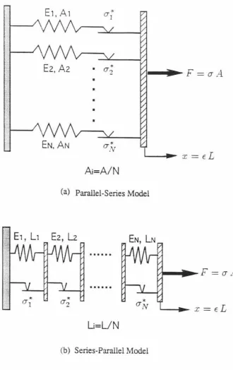
composed of a set of N elements connected in parallel, each of which consists of a linear spring with stiffness k/N in series with a slip element (Coulomb damper) of strength ri / N , as shown in Fig. 3.4. Each element in the assemblage is thus an ideal elasto-plastic element that has a force-deflection behavior as described in Fig. 3.1(a). The DEM has been considered as physically motivated, as many real materials or mechanical systems can be thought of as having a similar structure. For example, real materials may have a crystalline structure that is made up of a distribution of slip-planes or dislocations of different slip strengths. Therefore, the behavior of such a class of models can be expected to be physically consistent, with-out exhibiting unrealistic characteristics. The restoring force of a DEM consisting of N elements can be found to be given by

(3.8)

for initial loading, where n is the number of elements in the yielding state. When the total number of elements N becomes very large, the summation in Eqn. (3.8) may be replaced by an integral so that Eqn. (3.8) becomes

i

kx

1

oo

r = r* </>(r*) dr*

+

k x </>(r*) dr*,

0 kx

(3.9)

where ¢(r*) dr* denotes the fraction of the total number of elements with strengths in the ranger* ~ ri ~ r*

+

dr* , and the yield-strength distribution function ¢(r*) satisfies

1

00

</>(r*) dr* = 1. (3.10)

(30)

in Eqn. (3.9), may not be efficient for numerical solutions. Thus, in practical ap-plications using the DEM, such as the system identification study performed by

Cifuentes and Iwan [9], one has to introduce a finite number of elements so that their response can be traced with reasonable computation effort. This would,

some-how, degrade the results of analysis (e.g., the hysteretic yielding response curves become non-smooth), and, moreover, make the parameter identification more dif -ficult, unless some additional assumptions are made regarding elements' behavior

so that the number of parameters involved in the model can be appropriately

re-duced. It is important to note that the DEMs actually fall within the general class

of Masing models whose behavior can be described by the Masing's hypothesis and

some extended rules [23]. This will be elucidated in the next section.

3.2.3 The General Class of Masing Models

3.2.3.1 Masing's Hypothsis and Extended Rules

In his original paper titled "Self Stretching and Hardening for Brass" [31], Masing asserted that if the force-displacement curve for a system at the initial

loading is described by

f(r,x)=O, (3.11)

were r is the restoring force and x the displacement of the system, then the unload -ing and reload-ing branches of the steady-state hysteretic response of the system are

geometrically similar to the initial loading curve except for a two-fold magnification,

and are described by

f(r - ro x- xo) = 0

2 ' 2 ' (3.12)

where

(x

0 ,

r

0 ) is the load reversal point for that particular loading branch. Note

that the function

f

should satisfy

f( -r, -x) = f(r, x) (3.13)

so that the initial force-deflection curve is symmetric about the origin. The above

assertion is usually referred to as Masing's hypothesis for steady-state cyclic

(31)

with some experimental observations of the Bauschinger effect occurring in some metals, which indicates that an initial plastic deformation in one direction reduces the resistance of the material with respect to a subsequent plastic deformation in

the opposite direction. This effect is usually attributed to the residual stresses left

in the material due to initial loading or to the anisotropy of the dislocation field

generated by loading processes [26]. Some properties of response behavior using Masing's hypothesis were summarized in [23] and are not reiterated here. One

major concern associated with the original Masing's hypothesis is that it is useful

only for steady-state cyclic response or loading between fixed limits. In the case of transient response, or loading between variable limits, the hypothesis was consid-ered to be of no help. However, Jayakumar [23] proposed an extension of Masing's hypothesis by stipulating two general hysteresis rules so that simple and physical behavior for transient hysteretic response can be obtained accordingly. The two rules are as follows:

Rule 1: Incomplete Loops

The equation of any hysteretic response curve, irrespective of steady-state or transient response, can be obtained simply by applying the original Masing rule to

the virgin loading curve using the latest point of loading reversal.

Consider, for example, the hysteretic loops shown in Fig. 3.6. If the virgin loading

curve OA is characterized by Eqn. (3.11), then applying Rule 1, the equation for

the branch curve CD will be

f

(

r -₂r c X -_' ₂Xc) = 0 _. (3.14)

Based on Eqn. (3.14), it is easy to show that if the reloading curve CD in Fig. 3.6 had been continued, it would have formed a closed hysteresis loop given by ABCDA.

Rule 2 : Completed Loops

The ultimate fate of an interior curve under continued loading or unloading is

such that once the interior curve crosses a curve described in a previous load cycle, the force-deformation curve follows that of the previous cycle.

(32)

An effective algorithm for numerical implementation of these extended Masing

rules was proposed by Thyagarajan [45], and this algorithm has been adopted in

the present study for response simulation of Masing models. In the algorithm, two load reversal points are removed from the memory list each time an interior

response curve crosses a curve described in a previous load cycle. One important result regarding the extended Masing rules is that the hysteretic behavior of a

DEM can be completely described by these rules without the need of tracing each

element's behavior. This has been proven by Jayakumar [23], who then proposed a general class of Masing models based on the extended Masing rules. To specify any particular model in this class, only its initial loading curve need be prescribed. The

complete hysteretic behavior of this general class of Masing models is then governed

by the extended rules 1 and 2 stated above.

Thus, aDEM can be equivalent to a general Masing model if the yield-strength distribution function ¢(r*), along with the stiffness constant k, of aDEM is chosen to match identically the initial loading curve for a general Masing model.

Con-sidering the equivalence of the two classes of models, one may prefer to use the

Masing models in practical applications, since the implementation of the Masing models is much simpler and more efficient than that of the DEMs. In particular, for

applications, such as system identification studies, that involve a large number of iterations of model response calculations, numerical efficiency is of vital importance in the choice of models, provided that the models do not exhibit any unrealistic or unstable behavior.

3.2.3.2 A Special Class of Masing Models

Following the general class of Masing models based on the extended Masing rules for transient response, Jayakumar and Beck [24] proposed a special class of Masing models by defining the restoring force-deformation relation for the virgin loading by the differential equation:

(3.15)

(33)

The parameters k and ru, respectively, represent the small-amplitude stiffness and the ultimate strength of the system to be modeled. The additional parameter n is introduced to model different degrees of smoothness around the yielding point, as shown in Fig. 3.7, where the case n--+ oo corresponds to the elasto-perfectly plastic model.

Based on the extended Masing rules, the force-deformation relation for any loading branch other than the virgin curve is thus defined by the following equation:

dr = k [1

-I

r - ro

In].

dx

2ru (3.16)

It should be noted that the structure of Eqn. (3.15) is similar to those used in many other models, including the Bouc-Wen, Ozdemir, and the simple endochronic models as introduced in Section 3.2. The major difference, though, is that for the special class of Masing models, Eqn. (3.15) is used only for virgin loading, not for the complete response history. The major advantage of introducing the supplementary hysteresis rules is that unrealistic cyclic behavior, such as unstable drift and nonclosure of hysteresis loops, can be eliminated.

This special class of models has been applied to system identification studies using inelastic pseudo-dynamic test data from a full-scale, six-story steel structure [24]. Even though a shear-building approximation was used in the modeling of the pseudo-dynamic test structure, good results obtained confirm the applicability of this class of hysteretic models to real structures. Some other special classes of Mas-ing models can also be proposed by choosing particular yield-strength distribution functions that satisfy Eqn. (3.10) and are characterized by suitable parameters. More will be said about this in the next section when the Masing models are ex-tended to account for the effects of strength and stiffness degradation.

3.3 Modeling of Degrading Hysteretic Systems

(34)

1) a loss of stiffness, which often results in an increase in the period of vibration,

2) a decrease in energy dissipation capacity,

3) a redistribution of internal forces, and 4) a reduction of ultimate strength.

Iemura and Jennings [18] have observed a stiffness degradation of more than

50%, based on the change of natural frequencies, by analyzing measurements from Millikan Library Building, located on the campus of California Institute of

Tech-nology, Pasadena, during the 1971 San Fernando earthquake. Therefore, structures

under strong environmental loads are expected to undergo nonlinear and

time-dependent degrading behavior. The analysis of such a problem is also important

in many other engineering areas, such as damage detection of space structures and

adaptive control of mechanical systems. The difficulty of modeling such hysteretic

degrading systems often lies in the fact that the exact nature of system degradation

depends not only on the structural materials but also on the detailed configurations,

and may vary considerably from system to system.

In this section, we will investigate the extension of the three types of one-dimensional hysteretic models described in the previous section to account for the

effects of deterioration observed in actual structural systems.

3.3.1 The Degrading Bouc-Wen Model

The versatile nature and simple analytic form of the Bouc-Wen model as

de-scribed by Eqn. (3.1) has attracted considerable attention from researchers in many related engineering fields. To make it even more general, Wen [52] extended the original model to include the effects of strength and stiffness deterioration. The modeling technique for incorporating system degradation consists of the introduc-tion of more control parameters and the selection of a response index on which the

rate of degradation is based. Wen extended Eqn. (3.1) to

(3.17)

where the two additional parameters rJ and v are introduced to control the stiffness

(35)

properly-chosen response index. In his original work, Wen also chose the

parame-ter A that controls the response amplitude to be a function of the response index

so that the model thus defined can achieve the maximum flexibility in modeling

general hysteretic behavior, including strain hardening or softening effects. The

response index on which the degrading parameters depend should be able to reflect

the severity and duration of the system response and is usually selected as the

max-imun displacement experienced by the model or the total energy dissipated through

hysteresis, depending on the specific structural system being modeled. Fig. 3.8

il-lustrates the effects of the degrading parameters on the model behavior, in which

the parameters A, 'fJ, v are defined as

A( e) = Ao-DA e,

'fJ(e)

=

1.0

+

8₇₁e, v(e)

=

1.0

+

Ov e,

where e denotes the accumulation of the dissipated hysteretic energy, and the 8's

are constants specified for the desired rate of degradation. Although the degrading

hysteretic model given by Eqn. (3.17) is general and flexible, and it has

closed-form stochastic equivalent linearization coefficients as well, it is in general

over-parameterized, which causes difficulties in choosing appropriate parameter values

because of lack of identifiability when the model is applied to system identification

studies. For example, as reported in the paper by Sues et al. [42], the parameters

identified from simulated response can have values very different from those

origi-nally used in the simulation of response histories, though the response generated by

the identified parameters was found to be almost identical with that generated with

the original set of parameters. Another problem with the model is, as stated earlier

in this chapter, that it exhibits unrealistic drift behavior when subjected to small

cyclic excitations, which leads to a violation of Drucker's postulates of stability.

3.3.2 A Class of Deteriorating Distributed-Element Models

In order to apply the physically-motivated Distributed-Element Model (DEM)

to practical structural problems encountered in earthquake engineering, Iwan and

Cifuentes [22] presented a class of deteriorating DEMs for the overall restoring force

(36)

same ensemble of linear springs and Coulomb slip elements as shown in Fig. 3.4;

however, some of the elements are allowed to "break" if the absolute value of the displacements of an element exceeds some value, say

J.LYi

,

J.L

~ 1, where

Yi

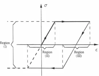
is the slip (yield) displacement of the element. Once the element "fails", it no longer contributes to the overall restoring force. Fig. 3.9 illustrates the restoring force diagram of a typical "breaking" element, and Fig. 3.10 shows an example of the overall response behavior of such a model subjected to a real earthquake excitation. Note that the parameter

J.L

acts as the maximum ductility ratio of an element defined as the ratio of maximum possible displacement response to the yield displacement of an element. It was also assumed for simplicity that all the elements of a model have the same value of J.L. This deteriorating model was shown to be capable of describing the major features of the restoring force behavior of concrete structures [22] while still maintaining the inherent simplicity of the original DEM. This model has also been applied to system identification studies of real structures using earthquake data [9] to assess the damage suffered by a structure and to predict its future performance.

Although satisfactory identification results were obtained using this special class of deteriorating DEMs, some additional assumptions were made in [9] pertain-ing to the relations among parameters and to the number of elements so that the actual number of parameters of the model was low enough for reliable identification.

(37)

3.3.3 A Class of Deteriorating Masing Models

3.3.3.1 General Formulation

We have mentioned in Section 3.2 the equivalence between the classes of DEMs

and Masing models such that a class of DEMs may be replaced by a class of Masing

models in system identification applications in which parameter identifiability is of

major concern. The extended Masing rules on which the behavior of the general

class of nondegrading Masing models are based provide an effective way of

imple-menting numerically the model behavior. In the case where degradation effects

are to be taken into account, can we still find some appropriate rules so that the

behavior of the DEMs can be found without the need of keeping track of elements'

behavior? This question is answered affirmatively in this section for the class of

maximum-displacement-controlled DEMs mentioned in the previous section.

To begin with, we propose a general formulation for modeling of degrading

systems. Following the integral formulation of the DEM, such as that given by

Eqn. (3.9), a damage index function a = a(r*,x)

t

can be introduced so that

at displacement x, the fraction of the total number of elements which are "un

-damaged" and with yield strengths in the range [r*, r*

+

dr*] can be denoted as

a(r*, x)</>(r*) dr* :j:. Thus, for initial loading, the restoring force can be represented

as

1

oo

1kx

r(x) = kx </>(r*)dr*

+

r*a(r*,x)</>(r*)dr*,

kx

0

(3.18)

where we assume that a( r*, x) = 1 for r*

2

kx, which means that elements that

are unyielded must be undamaged. The second term on the right-hand side of

Eqn. (3.18) is the contribution from elements that are yielded at deformation x,

and the first term denotes the contribution from elements that are still in the

elastic state for which a(·, ·) = 1.

t

In general, a can be a function of the history of x, not just x(t).

:j: (1-a) could be viewed as the fraction of elements in the yield range [r*, r*+dr*]

which have failed and completely lost their strength, or that (1-a) is the "average"

(38)

Similarly, for unloading from x0 , we have for -x0 ::; x::; x0 ,

1

oo ~kxo

r(x)=kx ¢>(r*)dr*+ [r*-k(xo-x)]a(r*,x)¢>(r*)dr*

k Xp k(xp-x) 2

k(xp- x)

+1

2

-r* a(r*, x) ¢>(r*) dr*, (3.19)

and for x

<

-xo,

l

oo 1-kx

r(x) = kx ¢>(r*)dr*

+

-r*a(r*,x)¢>(r*)dr*.

-kx 0

(3.20)

Very similar equations can also be derived for reloading. Equations (3.18), (3.19) and (3.20) can be differentiated with respect to x to get equations for the model "stiffness" as follows:

dr = k roo ¢>(r*)dr* +1kx r* aa(r*,x) ¢>(r*)dr*,

dx lkx 0 ax

(3.21)

for initial loading,

dr 1 oo jkxo

-d =k ¢>(r*)dr*+k a(r*,x)¢>(r*)dr*

X k k(x-xp)

Xp 2

k k(xp-x)

+

r Xp [r*-k(Xo- x)] aa(r* l X) ¢>(r*) dr* - 1 2

r* aa(T*, X) ¢>(r*) dr* l

J

~(xp-x) ax 0 ax

2

(3.22)

for unloading from xo with -xo ::; x ::; x0 , and

dr

=

kloo ¢>(r*)dr*- r-kx r* aa(r*,x) ¢>(r*)dr*,

dx -kx lo ax (3.23)

for unloading from xo with x

< -xo

.

We may note that the equations for r and dr / dx in the case of unloading from x0 with x

<

-x0 (Eqns. (3.20) and (3.23)) are the same as those for initial loading

in the negative direction (cf. Eqns. (3.18) and (3.21)). This is consistent with the extended Masing rule 2 regarding completed loops for transient response, as stated

(39)

choosing the damage index functions a. A specific example of choosing a as a

Heaviside step function will be given in the next section to illustrate the above formulation.