Munich Personal RePEc Archive
Robust linear static panel data models
using epsilon-contamination
Baltagi, Badi H. and Bresson, Georges and Chaturvedi,
Anoop and Lacroix, Guy
Syracuse University, USA, Université Paris II, France, University of
Allahabad, India, Université Laval, Canada
14 November 2014
Robust linear static panel data models
using
ε
-contamination
Badi H. Baltagi∗ Syracuse University, USA
Georges Bresson
Universit´e Paris II, France
Anoop Chaturvedi
University of Allahabad, India
Guy Lacroix
Universit´e Laval, Canada
November 14, 2014
Abstract
The paper develops a general Bayesian framework for robust linear static panel data models using ε-contamination. A two-step approach is employed to derive the conditional type-II maximum likelihood (ML-II) posterior distribution of the coefficients and individual effects. The ML-II posterior densities are weighted averages of the Bayes estimator under a base prior and the data-dependent empirical Bayes estimator. Two-stage and three stage hier-archy estimators are developed and their finite sample performance is investigated through a series of Monte Carlo experiments. These include standard random effects as well as Mundlak-type, Chamberlain-type and Hausman-Taylor-type models. The simulation results underscore the relatively good performance of the three-stage hierarchy estimator. Within a single theoretical framework, our Bayesian approach encompasses a variety of specifications while conventional methods require separate estimators for each case. We illustrate the per-formance of our estimator relative to classic panel estimators using data on earnings and crime.
Keywords: ε-contamination, hyperg-priors, type-II maximum likelihood posterior density, panel data, robust Bayesian estimator, three-stage hierarchy.
JEL classification: C11, C23, C26.
∗
Corresponding author. Department of Economics and Center for Policy Research, 426 Eggers Hall, Syracuse
Uni-versity, Syracuse, NY 13244–1020 USA. Tel.: +1 315 443 1630.E-mail: [email protected](B.H. Baltagi),
[email protected](G. Bresson),[email protected](A. Chaturvedi),[email protected]
(G. Lacroix).
1
Introduction
The choice of which classic panel data estimator to employ for a linear static regression model depends upon the hypothesized correlation between the individual effects and the regressors. Random effects assume that the regressors are uncorrelated with the indi-vidual effects, while fixed effects assume that all of the regressors are correlated with the individual effects (see Mundlak (1978) and Chamberlain (1980)). When a subset of the re-gressors are correlated with the individual effects, one employs the instrumental variables estimator of Hausman and Taylor (1981). In contrast, a Bayesian needs to specify the dis-tributions of the priors (and the hyperparameters in hierarchical models) to estimate the model. It is well-known that Bayesian models can be sensitive to misspecification of these distributions. In empirical analyses, the choice of specific distributions is often made out of convenience. For instance, conventional proper priors in the normal linear model have been based on the conjugate Normal-Gamma family essentially because all the marginal likelihoods have closed-form solutions. Likewise, statisticians customarily assume that the variance-covariance matrix of the slope parameters follow a Wishart distribution because it is convenient from an analytical point of view.
Often the subjective information available to the experimenter may not be enough for correct elicitation of a single prior distribution for the parameters, which is an essential requirement for the implementation of classical Bayes procedures. The robust Bayesian approach relies upon a class of prior distributions and selects an appropriate prior in a data dependent fashion. An interesting class of prior distributions suggested by Berger (1983, 1985) is the ε-contamination class, which combines the elicited prior for the pa-rameters, termed as base prior, with a possible contamination class of prior distributions and implements Type II maximum likelihood (ML-II) procedure for the selection of prior distribution for the parameters. The primary advantage of using such a contamination class of prior distributions is that the resulting estimator obtained by using ML-II proce-dure performs well even if the true prior distribution is away from the elicited base prior distribution.
The objective of our paper is to propose a robust Bayesian approach to linear static panel data models. This approach departs from the standard Bayesian model in two ways. First, we consider theε-contamination class of prior distributions for the model parameters (and for the individual effects). The base elicited prior is assumed to be contaminated and the contamination is hypothesized to belong to some suitable class of prior distributions. Second, both the base elicited priors and theε-contaminated priors use Zellner’s (1986)g -priors rather than the standard Wishart distributions for the variance-covariance matrices. The paper contributes to the panel data literature by presenting a general robust Bayesian framework. It encompasses the above mentioned conventional frequentist specifications and their associated estimation methods and is presented in Section 2.
In Section 3 we derive the Type II maximum likelihood posterior mean and the variance-covariance matrix of the coefficients in a two-stage hierarchy model. We show that the ML-II posterior mean of the coefficients is a shrinkage estimator,i.e., a weighted average of the Bayes estimator under a base prior and the data-dependent empirical Bayes estimator. Furthermore, we show in a panel data context that theε-contamination model is capable of extracting more information from the data and is thus superior to the classical Bayes estimator based on a single base prior.
Section 5 investigates the finite sample performance of the robust Bayesian estimators through extensive Monte Carlo experiments. These include the standard random effects model as well as Mundlak-type, Chamberlain-type and Hausman-Taylor-type models. We find that the three-stage hierarchy model outperforms the standard frequentist estimation methods. Section 6 compares the relative performance of the robust Bayesian estimators and the standard classical panel data estimators with real applications using panel data on earnings and crime. We conclude the paper in Section 7.
2
The general setup
Let us specify a Gaussian linear mixed model:
yit=Xit′β+W ′
itbi+εit ,i= 1, ..., N ,t= 1, ..., T, (1)
whereX′
it is a (1×K1) vector of explanatory variables excluding the intercept, andβ is
a (K1×1) vector of slope parameters. Furthermore, let Wit′ denote a (1×K2) vector of
covariates andbi a (K2×1) vector of parameters. The subscriptiofbi indicates that the
model allows for heterogeneity on theW variables. Finally,εitis a remainder term assumed
to be normally distributed, i.e. εit ∼N 0, τ−1. The distribution of εit is parametrized
in terms of its precisionτ rather that its variance σ2
ε(= 1/τ).In the statistics literature,
the elements ofβ do not differ acrossi and are referred to as fixed effects whereas thebi
are referred to asrandom effects.1 The resulting model in (1) is a Gaussian mixed linear model. This terminology differs from the one used in econometrics. In the latter, the
bi’s are treated either as random variables, and hence referred to as random effects, or as
constant but unknown parameters and hence referred to as fixed effects. In line with the econometrics terminology, wheneverbi is assumed to be correlated (uncorrelated) with all
theX′
its, they will be termed fixed (random) effects.2
In the Bayesian context, following the seminal papers of Lindley and Smith (1972) and Smith (1973), several authors have proposed a very general three-stage hierarchy framework to handle such models (see, e.g., Chib and Carlin (1999), Greenberg (2008), Koop (2003), Chib (2008), Zheng et al. (2008), Rendon (2013)):
First stage : y=Xβ+W b+ε, ε∼N(0,Σ),Σ =τ−1I N T
Second stage : β ∼N(β0,Λβ) and b∼N(b0,Λb)
Third stage : Λ−1b ∼W ish(νb, Rb) and τ ∼G(·).
(2)
wherey is (N T ×1),X is (N T ×K1),W is (N T ×K2),εis (N T ×1), and Σ =τ−1IN T
is (N T ×N T). The parameters depend upon hyperparameters which follow random dis-tributions. The second stage (also called fixed effects model in the Bayesian literature) updates the distribution of the parameters. The third stage (also called random effects model in the Bayesian literature) updates the distribution of the hyperparameters. As stated by Smith (1973, pp. 67) “for the Bayesian model the distinction between fixed, random and mixed models, reduces to the distinction between different prior assignments in the second and third stages of the hierarchy”. In other words, thefixed effects model is a model that does not have a third stage. The random effects model simply updates the distribution of the hyperparameters. The precisionτ is assumed to follow a Gamma dis-tribution and Λ−1
b is assumed to follow a Wishart distribution withνb degrees of freedom
and a hyperparameter matrix Rb which is generally chosen close to an identity matrix.
1
See Lindley and Smith (1972), Smith (1973), Laird and Ware (1982), Chib and Carlin (1999), Green-berg (2008), and Chib (2008) to mention a few.
2
In that case, the hyperparameters only concern the variance-covariance matrix of the b
coefficients3 and the precision τ. As is well-known, Bayesian models may be sensitive to possible misspecification of the distributions of the priors. Conventional proper priors in the normal linear model have been based on the conjugate Normal-Gamma family because they allow closed form calculations of all marginal likelihoods. Likewise, rather than speci-fying a Wishart distribution for the variance-covariance matrices as is customary, Zellner’s
g-prior (Λβ = (τ gX′X)−1 for β or Λb = (τ hW′W)−1 forb) has been widely adopted
be-cause of its computational efficiency in evaluating marginal likelihoods and bebe-cause of its simple interpretation as arising from the design matrix of observables in the sample. Since the calculation of marginal likelihoods using a mixture of g-priors involves only a one dimensional integral, this approach provides an attractive computational solution that made the originalg-priors popular while insuring robustness to misspecification of g (see Zellner (1986) and Fernandez, Ley and Steel (2001) to mention a few). To guard against mispecifying the distributions of the priors, many suggest considering classes of priors (see Berger (1985)).
3
The robust linear static model in the two-stage hierarchy
Following Berger (1985), Berger and Berliner (1984, 1986), Zellner (1986), Moreno and Pericchi (1993), Chaturvedi (1996), Chaturvedi and Singh (2012) among others, we con-sider theε-contamination class of prior distributions for (β, b, τ):
Γ ={π(β, b, τ |g0, h0) = (1−ε)π0(β, b, τ |g0, h0) +εq(β, b, τ |g0, h0)}. (3)
π0(·) is then the base elicited prior,q(·) is the contamination belonging to some suitable
classQof prior distributions, 0≤ε≤1 is given and reflects the amount of error in π0(·).
The precisionτ is assumed to have a vague priorp(τ)∝τ−1, 0< τ <∞. π
0(β, b, τ |g0, h0)
is the base prior assumed to be a specificg-prior with
β ∼ Nβ0ιK1,(τ g0ΛX)
−1 with Λ
X =X′X
b ∼ Nb0ιK2,(τ h0ΛW)
−1
with ΛW =W′W.
(4)
β0, b0, g0 and h0 are known scalar hyperparameters of the base prior π0(β, b, τ |g0, h0).
The probability density function (henceforth pdf) of the base priorπ0(.) is given by:
π0(β, b, τ |g0, h0) =p(β |b, τ, β0, b0, g0, h0)×p(b|τ, b0, h0)×p(τ). (5)
The possible class of contaminationQ is defined as:
Q=
q(β, b, τ |g0, h0) =p(β |b, τ, βq, bq, gq, hq)×p(b|τ, bq, hq)×p(τ)
with 0< gq≤g0, 0< hq≤h0
(6)
with
β ∼ NβqιK1,(τ gqΛX)
−1
b ∼ NbqιK2,(τ hqΛW)
−1, (7)
whereβq, bq,gq andhq are unknown. The ε-contamination class of prior distributions for
(β, b, τ) is then conditional on knowng0 andh0 and two estimation strategies are possible:
3
Note that in (2), the prior distribution ofβ andbare assumed to be independent, so Var[θ] is block-diagonal withθ = (β′, b′)′. The third stage can be extended by adding hyperparameters on the prior
mean coefficientsβ0 andb0 and on the variance-covariance matrix of theβcoefficients: β0∼N(β00,Λβ0),
b0 ∼N(b00,Λb0) and Λ
−1
β ∼W ish(νβ, Rβ) (see for instance, Greenberg (2008), Hsiao and Pesaran (2008),
1. a one-step estimation of the ML-II posterior distribution4 of β,band τ;
2. or a two-step approach as follows:
(a) Let y∗ = (y−W b). Derive the conditional ML-II posterior distribution of β
given the specific effects b.
(b) Let ye = (y−Xβ). Derive the conditional ML-II posterior distribution of b
given the slope coefficients β.
We use the two-step approach because it simplifies the derivation of the predictive densities (or marginal likelihoods). In the one-step approach the pdf of y and the pdf of the base priorπ0(β, b, τ |g0, h0) need to be combined to get the predictive density. It
thus leads to a complicated expression whose integration with respect to (β, b, τ) may be difficult. Using a two-step approach we can integrate first with respect to (β, τ) givenband then, conditional on β, we can next integrate with respect to (b, τ). Thus, the marginal likelihoods (or predictive densities) corresponding to the base priors are:
m(y∗
|π0, b, g0) = ∞
Z
0
Z
RK1
π0(β, τ |g0)×p(y∗ |X, b, τ) dβ dτ
and
m(ey|π0, β, h0) = ∞
Z
0
Z
RK2
π0(b, τ |h0)×p(ye|W, β, τ) db dτ,
with
π0(β, τ |g0) =
τ g0 2π
K1 2
τ−1|Λ
X|1/2exp
−τ g0
2 β−β0ιK1)
′
ΛX(β−β0ιK1)
,
π0(b, τ |h0) =
τ h0
2π
K2 2
τ−1|Λ
W|1/2exp
−τ h0
2 (b−b0ιK2)
′
ΛW(b−b0ιK2)
.
Solving these equations is considerably easier than solving the equivalent expression in the one-step approach.
3.1 The first step of the robust Bayesian estimator
Let y∗ = y−W b. Combining the pdf of y∗ and the pdf of the base prior, we get the
predictive density corresponding to the base prior5:
m(y∗
|π0, b, g0) = ∞
Z
0
Z
RK1
π0(β, τ |g0)×p(y∗|X, b, τ) dβ dτ (8)
= He
g0
g0+ 1
K1/2 1 +
g0
g0+ 1
R2 β0 1−R2
β0
!!−N T
2
with
e
H= Γ
N T 2
π(N T2 )v(b)(
N T
2 )
, (9)
4
“We consider the most commonly used method of selecting a hopefully robust prior inΓ, namely choice of that prior π which maximizes the marginal likelihoodm(y|π) overΓ. This process is called Type II maximum likelihood by Good (1965)”(Berger and Berliner (1986), page 463.)
R2β0 = (bβ(b)−β0ιK1)
′Λ
X(bβ(b)−β0ιK1) (βb(b)−β0ιK1)
′Λ
X(βb(b)−β0ιK1) +v(b)
, (10)
b
β(b) = Λ−1
X X
′y∗ and v(b) = (y∗−Xβb(b))′(y∗−Xbβ(b)) and where Γ (·) is the Gamma
function.
Similarly, for the distributionq(β, τ |g0, h0)∈Qfrom the classQof possible
contam-ination distribution, we can obtain the predictive density corresponding to the contami-nated prior:
m(y∗
|q, b, g0) =He
gq
gq+ 1
K1 2
1 +
gq
gq+ 1
R2 βq 1−R2βq
!!−N T2
, (11)
where
Rβ2q = (bβ(b)−βqιK1)
′
ΛX(bβ(b)−βqιK1) (bβ(b)−βqιK1)
′Λ
X(bβ(b)−βqιK1) +v(b)
. (12)
As the ε-contamination of the prior distributions for (β, τ) is defined by π(β, τ |g0) =
(1−ε)π0(β, τ |g0) +εq(β, τ |g0), the corresponding predictive density is given by:
m(y∗
|π, b, g0) = (1−ε)m(y∗ |π0, b, g0) +εm(y∗ |q, b, g0) (13)
and
sup
π∈Γ
m(y∗
|π, b, g0) = (1−ε)m(y∗ |π0, b, g0) +εsup q∈Q
m(y∗
|q, b, g0). (14)
The maximization of m(y∗
|π, b, g0) requires the maximization of m(y∗ |q, b, g0) with
respect toβq and gq. The first-order conditions lead to
b
βq= ι′
K1ΛXιK1 −1
ι′
K1ΛXbβ(b) (15)
and
b
gq = min (g0, g∗) (16)
withg∗
= max
(N T −K1)
K1
(bβ(b)−bβqιK1)
′Λ
X(bβ(b)−βbqιK1)
v(b) −1
!−1
,0 = max
(N T −K1)
K1 R 2 b βq 1−R2
b
βq −1
−1 ,0 .
Denote supq∈Qm(y∗ |q, b, g0) =m(y∗|bq, b, g0). Then
m(y∗
|q, b, gb 0) =He
b
gq
b
gq+ 1
K1 2 1 + b gq b
gq+ 1
R2
b
βq 1−R2
b βq
−N T2
. (17)
Letπ∗
0(β, τ |g0) denote the posterior density of (β, τ) based upon the prior π0(β, τ|g0).
Also, letq∗(β, τ |g
0) denote the posterior density of (β, τ) based upon the priorq(β, τ |g0).
The ML-II posterior density of β is thus given by:
b
π∗
(β|g0) = ∞
Z
0
b
π∗
(β, τ |g0)dτ
= bλβ,g0
∞
Z
0
π∗
0(β, τ |g0)dτ+
1−λbβ,g0 Z∞
0
q∗
(β, τ |g0)dτ
= bλβ,g0π
∗
0(β |g0) +
1−bλβ,g0
b
q∗
with
b
λβ,g0 =
1 + ε 1−ε
b
gq
b
gq+1
g0
g0+1
K1/2
1 + g0
g0+1
R2
β0
1−R2
β0
1 + bgq
b
gq+1
R2 b βq 1−R2 b βq ! N T 2 −1 . (19)
Note thatλbβ,g0 depends upon the ratio of the R
2
β0 and R
2
βq but primarily on the sample sizeN T. Indeed, bλβ,g0 tends to 0 when R
2 β0 > R
2
βq and bλβ,g0 tends to 1 whenR
2 β0 < R
2 βq irrespective of the model fit (i.e, the absolute values of R2β0 or R2βq). Only the relative values ofR2
βq and R
2
β0 matter. It can be shown that π∗
0(β |g0) is the pdf (see the Appendix) of a multivariate t
-distribution with mean vector β∗(b |g0), variance-covariance matrix
ξ0,βM0−,β1
N T−2
and de-grees of freedom (N T) with
M0,β =
(g0+ 1)
v(b) ΛX andξ0,β= 1 +
g0
g0+ 1
R2 β0 1−R2
β0 !
. (20)
β∗(b|g0) is the Bayes estimate ofβ for the prior distributionπ0(β, τ) :
β∗(b|g0) =
b
β(b) +g0β0ιK1
g0+ 1
. (21)
Likewise qb∗(β) is the pdf of a multivariate t-distribution with mean vector bβ
EB(b|g0),
variance-covariance matrix
ξq,βMq,β−1
N T−2
and degrees of freedom (N T) with
ξq,β= 1 +
b
gq
b
gq+ 1
R
2
b
βq 1−R2
b
βq
and Mq,β =
( b
gq+ 1)
v(b)
ΛX, (22)
wherebβEB(b|g0) is the empirical Bayes estimator ofβ for the contaminated prior
distri-butionq(β, τ) given by: b
βEB(b|g0) =
b
β(b) +bgqbβqιK1 b
gq+ 1
. (23)
The mean of the ML-II posterior density ofβ is then:
b
βM L−II = E[bπ ∗
(β|g0)] (24)
= bλβ,g0E[π
∗
0(β |g0)] +
1−bλβ,g0
E[bq∗
(β|g0)]
= bλβ,g0β∗(b|g0) +
1−bλβ,g0
b
βEB(b|g0).
The ML-II posterior mean of β, given b and g0 is a weighted average of the Bayes
esti-mator β∗(b | g0) under base prior g0 and the data-dependent empirical Bayes estimator
b
βEB(b|g0). If the base prior is consistent with the data, the weight bλβ,g0 → 1 and the ML-II posterior mean ofβ gives more weight to the posteriorπ∗
0(β|g0) derived from the
elicited prior. In this caseβbM L−II is close to the Bayes estimatorβ∗(b|g0). Conversely, if
the base prior is not consistent with the data, the weightbλβ,g0 →0 and the ML-II posterior mean ofβ is then close to the posterior bq∗(β|g
0) and to the empirical Bayes estimator
b
the data is what makes it superior to the classical Bayes estimator based on a single base prior.
The ML-II posterior variance-covariance matrix ofβ is given by (see Berger (1985) p. 207):
V arβbM L−II=λbβ,g0V ar[π
∗
0(β |g0)] +
1−bλβ,g0
V ar[qb∗
(β |g0)]
+bλβ,g0
1−bλβ,g0 β∗(b|g0)−bβEB(b|g0) β∗(b|g0)−bβEB(b|g0) ′
=λbβ,g0 ξ
0,β
N T −2
v(b)
g0+ 1
Λ−1
X (25)
+1−bλβ,g0
ξq,β
N T −2
v(b) b
gq+ 1
Λ−1X
+bλβ,g0
1−bλβ,g0 β∗(b|g0)−bβEB(b|g0) β∗(b|g0)−bβEB(b|g0)
′
.
3.2 The second step of the robust Bayesian estimator
Letey=y−Xβ. Moving along the lines of the first step, the ML-II posterior density ofb
is given by:
b
π∗
(b|h0) =bλb,h0π
∗
0(b|h0) +
1−bλb,h0
b
q∗
(b|h0)
with
b
λb,h0 = 1 +
ε
1−ε
b h b h+1 h0
h0+1
K2/2
1 + h0
h0+1
R2
b0
1−R2
b0
1 +bbh
h+1
R2
bbq
1−R2
bbq N T 2 −1 , (26) where
Rb20 = (bb(β)−b0ιK2)
′Λ
W(bb(β)−b0ιK2) (bb(β)−b0ιK2)
′Λ
W(bb(β)−b0ιK2) +v(β)
, (27)
Rb2
bq =
(bb(β)−bbqιK2)
′Λ
W(bb(β)−bbqιK2) (bb(β)−bbqιK2)
′Λ
W(bb(β)−bbqιK2) +v(β)
,
withbb(β) = Λ−1
WW
′
e
y andv(β) = (ey−Wbb(β))′(
e
y−Wbb(β)),
bbq= ι′K2ΛWιK2 −1
ι′
K2ΛWbb(β) (28)
and
bhq= min (h0, h∗) (29)
withh∗
= max
(N T −K2)
K2
(bb(β)−bbqιK2)
′
ΛW(bb(β)−bbqιK2)
v(β) −1
!−1 ,0 = max
(N T −K2)
K2 R 2 b bq 1−R2
bbq −1
−1 ,0 . π∗
0(b|h0) is the pdf of a multivariatet-distribution with mean vector b∗(β |h0),
variance-covariance matrix
ξ0,bM−
1 0,b
N T−2
and degrees of freedom (N T) with
M0,b=
(h0+ 1)
v(β) ΛW and ξ0,b= 1 +
h0
h0+ 1
(b
b(β)−b0ιK2)
′
ΛW(bb(β)−b0ιK2)
b∗(β |h0) is the Bayes estimate of bfor the prior distribution π0(b, τ |h0) :
b∗(β |h0) =
bb(β) +h0b0ιK2
h0+ 1
. (31)
q∗(b|h
0) is the pdf of a multivariatet-distribution with mean vectorbbEB(β |h0),
variance-covariance matrix
ξ1,bM1−,b1
N T−2
and degrees of freedom (N T) with
ξ1,b= 1 +
b
hq
b
hq+ 1
!
(bb(β)−bbqιK2)
′
ΛW(bb(β)−bbqιK2)
v(β) and M1,b =
bh+ 1
v(β) !
ΛW (32)
and wherebbEB(β|h0) is the empirical Bayes estimator of b for the contaminated prior
distributionq(b, τ |h0) :
bbEB(β |h0) =
b
β(b) +bhqbbqιK2 bhq+ 1
. (33)
The mean of the ML-II posterior density ofbis hence given by:
bbM L−II =bλbb∗(β |h0) +
1−bλβ
bbEB(β|h0) (34)
and the ML-II posterior variance-covariance matrix ofbis given by:
V arbbM L−II
=bλb,h0
ξ0,b
N T −2
v(β)
h0+ 1
Λ−1W (35)
+1−bλb,h0
ξ1,b
N T −2
v(β) bhq+ 1
! Λ−1
W
+bλb,h0
1−bλb,h0 b∗(β |h0)−bbEB(β |h0) b∗(β |h0)−bbEB(β |h0) ′
.
As our estimator is a shrinkage estimator, it is not necessary to draw thousands of multi-variatet-distributions to compute the mean and variance after burning draws. We can use an iterative shrinkage approach as suggested by Maddala et al. (1997) (see also Baltagi et al. (2008)) to compute the ML-II posterior mean and variance-covariance matrix of β
andb.
4
The robust linear static model in the three-stage
hierar-chy
As stressed earlier, the Bayesian literature introduces a third stage in the hierarchical model in order to discriminate betweenfixed effects andrandom effects. Hyperparameters can be defined for the mean and the variance-covariance ofb(and sometimesβ). Our ob-jective in this paper is to consider a contamination class of priors to account for uncertainty pertaining to the base priorπ0(β, b, τ),i.e., uncertainty about the prior means of the base
prior. Consequently, assuming hyper priors for the means β0 and b0 of the base prior is
tantamount to assuming the mean of the base prior to be unknown, which is contrary to our initial assumption. Following Chib and Carlin (1999), Greenberg (2008), Chib (2008), Zhenget al. (2008) among others, hyperparameters only concern the variance-covariance matrix of thebcoefficients. Because we use g-priors at the second stage forβ andb,g0 is
Zellner and Siow (1980) proposed a Cauchy prior on g which is not as popular as the
g-prior since closed form expressions for the marginal likelihoods are not available. More recently, and as an alternative to the Zellner-Siow’s prior, Lianget al.(2008) (see also Cui and George (2008)) have proposed a Pareto type II hyper-gprior whose pdf is defined as:
p(g) = (k−2)
2 (1 +g)
−k2
,g >0, (36)
which is a proper prior fork >2. One advantage of the hyper-gprior is that the posterior distribution ofg, given a model, is available in closed form. Unfortunately, the normalizing constant is a Gaussian hypergeometric function and a Laplace approximation is usually required to compute the integral of its representation for large samples, N T, and large
R2. Liang et al. (2008) have shown that the best choices fork are given by6 2 < k≤ 4.
Maruyama and George (2011, 2014) proposed a generalized hyper-g prior:
p(g) = g
c−1(1 +g)−(c+d)
B(c, d) ,c >0, d >0, (37)
whereB(·) is the Beta function. This Beta-prime (or Pearson Type VI) hyper prior forgis a generalization of the Pareto type II hyper-gprior since the expression in (36) is equivalent to that in (37) whenc= 1. In that specific case,d= (k−22).Using the generalized hyper-g
prior specification, the three-stage hierarchy of the model can be defined as:
First stage : y∼N(Xβ+W b,Σ) , Σ =τ−1I
N T (38)
Second stage : β∼Nβ0ιK1,(τ g0ΛX)
−1 ,b∼Nb
0ιK2,(τ h0ΛW)
−1
Third stage : h0 ∼β′(c, d) →p(h0) =
hc−1
0 (1 +h0)−(c+d)
B(c, d) ,c >0, d >0.
As our objective is to account for the uncertainty about the prior means of the base prior
π0(β, b, τ), we do not need to introduce an ε-contamination class of prior distributions
for the hyperparameters of the third stage of the hierarchy. Moreover, Berger (1985, p. 232) has stressed that the choice of a specific functional form for the third stage matters little. Sinha and Jayaraman (2010a, 2010b) studied a ML-II contaminated class of priors at the third stage of hierarchical priors using normal, lognormal and inverse Gaussian distributions to investigate the robustness of Bayes estimates with respect to possible misspecification at the third stage. Their results confirmed Berger’s (1985) assertion that the form of the second stage prior (the third stage of the hierarchy) does not affect the Bayes decision. Therefore we restrict the ε-contamination class of prior distributions to the first stage prior only (the second stage of the hierarchy,i.e., for (β, b, τ)).
The first step of the robust Bayesian estimator in the three-stage hierarchy is strictly similar to the one in the two-stage hierarchy. But the three-stage hierarchy differs from the two-stage hierarchy in that it introduces a generalized hyper-g prior on h0. The
unconditional predictive density corresponding to the base prior is then given by
m(ey|π0, β) = ∞
Z
0
m(ye|π0, β, h0)p(h0)dh0 (39)
= He
B(c, d)
1
Z
0
(ϕ)K22+c−1(1−ϕ)d−1 1 +ϕ R
2 b0 1−R2
b0
!!−N T
2
dϕ
6
which can be written as:
m(ye|π0, β) =
B(d,K2
2 +c)
B(c, d) He ×2F1
N T
2 ;
K2
2 +c;
K2
2 +c+d;−
R2 b0 1−R2b0
!!
, (40)
where2F1(.) is the Gaussian hypergeometric function (see Abramovitz and Stegun (1970)
and the Appendix). As shown by Lianget al. (2008), numerical overflow is problematic for moderate to largeN T and large R2b0. As the Laplace approximation involves an integral with respect to a normal kernel, we follow the suggestion of Liang et al. (2008) and develop an expansion after a change of variable given byφ= log h0
h0+1
(see the Appendix). Similar to the conditional predictive density corresponding to the contaminated prior onβ(see eq(17)), the unconditional predictive density corresponding to the contaminated prior onb is given by:
m(ye|q, βb ) =
∞
Z
0
m(ye|q, β, hb 0)p(h0)dh0 (41)
= He
B(c, d)×
h∗ Z 0 h0
h0+1
K2/2
1 + h0
h0+1
R2
b
bq
1−R2
b
bq
−N T2
×hc−1 0 1 1+h0 c+d dh0
+ He
B(c, d) h∗
h∗+ 1
K2 2
1 + h∗
h∗+ 1
R
2
bbq 1−R2
bbq
−N T
2 ×
∞
Z
h∗ hc−1
0
1 1 +h0
c+d
dh0.
m(ye|q, βb ) = (42)
= He
B(c, d)
2.hh∗+1∗ K2
2 +c
K2+2c
×F1
K2
2 +c; 1−d;N T2 ; K2
2 +c+ 1; h
∗
h∗+1;− h ∗
h∗+1
R2
b
bq
1−R2
b bq + h∗
h∗+1
K2 2
1 +h∗h+1∗
R2
bbq
1−R2
bbq
−N T
2
×
B(c, d)−
h∗
h∗+1 c
c
×2F1
c;d−1;c+ 1;h∗h+1∗
,
whereF1(.) is the Appell hypergeometric function (see Appell (1882), Slater (1966), and
Abramovitz and Stegun (1970)). m(ye|q, βb ) can also be approximated using the same clever transformation as in Liang et al. (2008) (see the Appendix).
We have shown earlier that the posterior density of (b, τ) for the base priorπ0(b, τ |h0)
in the two-stage hierarchy model is given by:
b
π∗
(b, τ |h0) =bλb,h0π
∗
0(b, τ |h0) +
1−λbb,h0
q∗
(b, τ |h0),
with
b
λb,h0 =
(1−ε)m(ey|π0, β, h0)
(1−ε)m(ye|π0, β, h0) +εm(ey|q, β, hb 0)
Hence, we can write
b
λb = ∞
Z
0
b
λb,h0p(h0)dh0 =
1 +
ε
1−ε
. m(ye|bq, β) m(ye|π0, β)
−1
. (43)
Therefore, under the base prior, the Bayes estimator of b in the three-stage hierarchy model is given by:
b∗(β) = ∞
Z
0
b∗(β |h0)p(h0)dh0 =
1
c+d
h
d·bb(β) +c·b0ιK2 i
.
Thus, under the contamination class of priors, the empirical Bayes estimator of bfor the three-stage hierarchy model is given by
bbEB(β) = ∞
Z
0
bbEB(β |h0)p(h0)dh0 (44)
= 1
B(c, d)
bb(β)
h∗
R
0
hc−1 0
1 1+h0
c+d+1
dh0+bbqιK2
h∗ R 0 hc 0 1 1+h0 c+d+1 dh0
+nbb(β)g∗1+1
+bbqιK2
h∗
h∗+1
o∞R
h∗ hc−1
0 1 1+h0 c+d dh0 = 1
B(c, d)
bb(β)
h∗
h∗+1 c
c ×2F1
c;−d;c+ 1;h∗h+1∗
+bbqιK2
h∗ h∗+1
c+1
c+1 ×2F1
c+ 1; 1−d;c+ 2;hh∗+1∗
+nbb(β)h∗1+1
+bbqιK2
h∗
h∗+1
o
×
B(c, d)−
h∗ h∗+1
c
c
×2F1
c;d−1;c+ 1;h∗h+1∗
and the ML-II posterior density ofbis given by:
b
π∗
(b) =
∞
Z
0
b
π∗
(b, τ)dτ =bλb ∞
Z
0
π∗
0(b, τ)dτ+
1−bλb
Z∞
0
q∗
(b, τ)dτ (45)
=bλbπ0∗(b) +
1−λbb
b
q∗
(b).
π∗
0(b) is the pdf of a multivariatet-distribution with mean vectorb∗(β), variance-covariance
matrix
ξ0,bM0−,b1
N T−2
and degrees of freedom (N T) with
M0,b=
(h0+ 1)
v(β) ΛW andξ0,b= 1 +
h0
h0+ 1
R2 b0 1−R2
b0 !
. (46)
b
q∗(b) is the pdf of a multivariate t-distribution with mean vector bb
EB(β),
variance-covariance matrix
ξq,bMq,b−1
N T−2
and degrees of freedom (N T) with
ξq,b= 1 +
b
hq
b
hq+ 1
! R
2
bbq 1−Rb2
bq
and Mq,b=
(bhq+ 1)
v(β) !
The mean of the ML-II posterior density ofbis thus given by
bbM L−II = E[bπ∗(b)] =bλbE[π∗0(b)] +
1−bλb
E[qb∗
(b)] (48)
= λbbb∗(β) +
1−bλb
bbEB(β)
and the ML-II posterior variance-covariance matrix ofbis given by:
V arbbM L−II
=bλb
ξ
0,b
N T −2.
v(β)
h0+ 1
Λ−1
W (49)
+1−λbb
ξq,b
N T −2
v(β) b
hq+ 1
! Λ−1
W
+λbb
1−bλb b∗(β)−bbEB(β) b∗(β)−bbEB(β)
′
.
The main differences with the two-stage hierarchy model relate to the definition of the Bayes estimator b∗(β), the empirical Bayes estimator bbEB(β) and the weights λbb (as
compared tob∗(β |h0),bbEB(β|h0) andbλb,h0). Once again, as our estimator is a shrinkage estimator, it is not necessary to draw thousands of multivariatet-distributions to compute the mean and the variance after burning draws. We can use an iterative shrinkage approach to calculate the ML-II posterior mean and variance-covariance matrix ofβ and b.
5
A Monte Carlo simulation study
5.1 The DGP of the Monte Carlo study
Following Baltagiet al. (2003, 2009) and Baltagi and Bresson (2012), consider the static linear model:
yit = x1,1,itβ1,1+x1,2,itβ1,2+x2,itβ2+Z1,iη1+Z2,iη2+µi+εit (50)
fori = 1, ..., N ,t= 1, ..., T
with
x1,1,it = 0.7x1,1,it−1+δi+ζit (51)
x1,2,it = 0.7x1,2,it−1+θi+ςit (52)
εit ∼ N 0, τ−1, (δi, θi, ζit, ςit)∼U(−2,2) (53)
and β1,1 = β1,2 =β2 = 1. (54)
1. For a random effects (RE) world, we assume that:
η1 = η2= 0 (55)
x2,it = 0.7x2,it−1+κi+uit , (κ, uit)∼U(−2,2) (56)
µi ∼ N 0, σ2µ
,ρ= σ
2 µ
σ2 µ+τ−1
= 0.3, 0.8. (57)
x1,1,it, x1,2,it and x2,it are assumed to be exogenous in that they are not correlated
2. For a Mundlak-type fixed effects (FE) world, we assume that:
η1 = η2= 0; (58)
x2,it = δ2,i+ω2,it ,δ2,i ∼N(mδ2, σ
2
δ2), ω2,it ∼N(mω2, σ
2
ω2); (59)
mδ2 = mω2 = 1, σ
2
δ2 = 8, σ
2
ω2 = 2; (60)
µi = x2,iπ+νi,νi∼N(0, σ2ν),x2,i=
1
T
T
X
t=1
x2,it; (61)
σν2 = 1, π= 0.8. (62)
x1,1,it and x1,2,it are assumed to be exogenous butx2,it is correlated with theµi and
we assume a constant correlation coefficient π= 0.8.
3. For a Chamberlain-type fixed effects (FE) world, we assume that:
η1 = η2= 0; (63)
x2,it = δ2,i+ω2,it ,δ2,i ∼N(mδ2, σ
2
δ2), ω2,it ∼N(mω2, σ
2
ω2); (64)
mδ2 = mω2 = 1, σ
2
δ2 = 8, σ
2
ω2 = 2; (65)
µi = x2,i1π1+x2,i2π2+...+x2,iTπT +νi,νi ∼N(0, σν2); (66)
σν2 = 1, πt= (0.8)T−t fort= 1, ..., T. (67)
x1,1,it and x1,2,it are assumed to be exogenous butx2,it is correlated with theµi and
we assume an exponential growth for the correlation coefficient πt.
4. For a Hausman-Taylor (HT) world, we assume that:
η1 = η2= 1; (68)
x2,it = 0.7x2,it−1+µi+uit ,uit ∼U(−2,2); (69)
Z1,i = 1, ∀i; (70)
Z2,i = µi+δi+θi+ξi,ξi ∼U(−2,2); (71)
µi ∼ N 0, σµ2
, andρ= σ
2 µ
σ2 µ+τ−1
= 0.3, 0.8. (72)
x1,1,it and x1,2,it and Z1,i are assumed to be exogenous while x2,it and Z2,i are
endogenous because they are correlated with the µi but not with theεit.
For each set-up, we vary the size of our panel. We choose several (N, T) pairs with
N = 100,500 and T = 5,10. We also choose N = 50, T = 20 as is typical for U.S. state panel data or country macro-panels. We generate the data by choosing initial values of
x1,1,it and x1,2,it to be zero. We generate x1,1,it, x1,2,it, εit, ζit, uit, ςit, ω2,it over T +T0
time periods and we drop the first T0(= 50) observations to reduce the dependence on
initial values. We also use the robust Bayesian estimators for the two-stage hierarchy (2S) and for the three-stage hierarchy (3S) withε= 0.5.
We must define the initial hyperparametersβ0, b0, g0, h0, τ for the initial distributions
of β ∼ Nβ0ιK1,(τ g0ΛX)
−1
and b ∼ Nb0ιK2,(τ h0ΛW)
−1
. While we can choose arbitrary values for β0, b0 and τ, the literature generally recommends the UIP, the RIC
and the BRIC for the g priors.7 In the normal regression case, and following Kass and
Wasserman (1995), the unit information prior (UIP) corresponds to g0 = h0 = 1/N T,
leading to Bayes factors that behave like the Bayesian Information Criterion (BIC). Fos-ter and George (1994) calibrated priors for model selection based on the Risk inflation
7We chose:
criterion (RIC) and recommended the use of g0 = 1/K12, h0 = 1/N2. Fern´andez et
al. (2001) recommended the BRIC (mix of BIC and RIC) using g0 = 1/max(N T, K12),
h0 = 1/max(N T, N2). We use the UIP since the RIC and the BRIC lead to very small
h0 priors.
For the three-stage hierarchy (3S), we need to choose the coefficients (c, d) of the generalized hyper-g priors. Liang et al. (2008) stressed that the best parameter for the Pareto type II distribution wask= 4 which corresponds toc=d= 1 for the Beta-prime distribution. In that case, the density is shaped as a hyperbola. In order to have the same shape under the UIP principle (i.e.,h0 close to 1/N T), we chosec= 0.1 andd= 1.
As our 2S and 3S estimators are shrinkage estimators (see eq.(24), eq.(34) for 2S and eq.(48) for 3S), we can use an iterative shrinkage approach as suggested by Maddalaet al. (1997) with only 50 iterations. For the three-stage hierarchy (3S), we could use Gaussian hypergeometric functions2F1 and Appel functionsF1with Laplace approximations but we
prefer to solve the integrals numerically with adaptive quadrature methods (see Davis and Rabinowitz (1984), Press et al. (2007)). For each experiment, we run 1000 replications and we compute the mean, standard error and root mean squared error (RMSE) of the coefficients.
5.2 The results of the Monte Carlo study
5.2.1 The random effects world
Let us rewrite our general model (2): y = Xβ +W b+ε, ε ∼ N(0,Σ), Σ = τ−1I N T as
y = Xβ +Zµµ+ε where Zµ = IN ⊗ιT is (N T ×N), ιT is a (T×1) vector of ones
and µ is a (N ×1) vector of idiosyncratic parameters. When W ≡ Zµ, the random
effects, µ∼N 0, σ2
µIN, are associated with the error termν=Zµµ+εwith Var (ν) =
σ2µ(IN⊗JT) +σε2IN T, where JT = ιTι′T and are estimated using Feasible Generalized
Least Squares (FGLS), (see Hsiao (2003) or Baltagi (2013)).
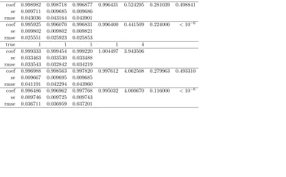
For the random effects world, we compare the standard FGLS estimator and our 2S and 3S estimators. In this specification, X = [x1,1, x1,2, x2], W =Zµ and b=µ. The results
in Table 1 are based on N = 100, T = 5 with ε= 0.5. The proportion of heterogeneity in the total variance, measured by the ratio of the variance of the individual effects to the total variance (ρ). This is allowed to be either 30% or 80%. Table 1 shows that the 2S and 3S robust estimators have good properties. The estimated coefficients are very close to the true values. More interestingly, their standard errors (se) are much smaller than those of FGLS. Indeed, the standard errors of the latter estimator are nearly twice as large as those of the 2S and 3S estimators. The bias and RMSE, however, are similar to those of FGLS. Estimates of the remainder variance (σ2
ε ≡τ−1) are the same and very
close to the true value (σε2 = 1). The robust 3S also correctly estimates the variance of the individual effects (σµ2). The 2S estimator yields unbiased coefficients but leads to a biased σ2
µ. The weights λβ and λb show the trade-off between the Bayes estimators
(β∗(b) and b∗(β)) and the empirical Bayes estimators (bβEB(b) and bbEB(β)). In the 2S
model,λβ = 28% (λb = 49%) which indicates that the empirical Bayes estimator bβEB(b)
(bbEB(β)) accounts for 72% (51%) of the weight in estimating the slope coefficients. In the
3S model, these ratios decrease considerably, from 22% to 11% for λβ when ρ increases
from 0.3 to 0.8. Furthermore, λb dramatically drops to zero. This means that only the
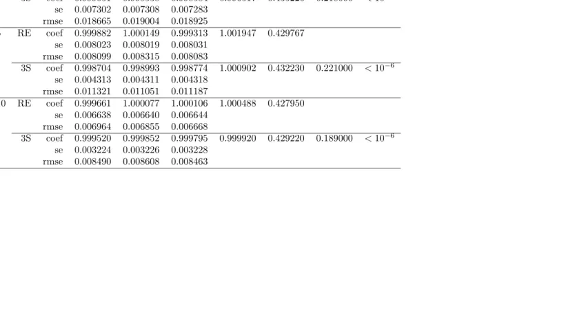
empirical Bayes estimator is used in the estimation of the individual effects (b≡µ). In addition, the standard errors of the 2S and 3S are now three times smaller and the estimate ofσµ2 of the 3S corresponds perfectly to the true value. These results are confirmed when we increase the size of the sample of the short panel (large N, small T) (see Appendix, Tables A2 and A3).8 Note that whenρincreases from 30% to 80%, the bias in the variance
of the individual effects (σ2
µ) is reduced and is smaller than −1.2% for N = 100,T = 10.
It is also smaller than−0.04% forN = 500, T = 10. Even for a macro-panel (N small, T
large), these results still hold (see Appendix Table A3 for N = 50,T = 20, ρ = 0.8 with
ε= 0.5) and the bias in the variance of the individual effects (σ2
µ) is smaller than −1.3%.
5.2.2 The Mundlak-type fixed effects world
In the fixed effects world, we allow the individual effects µ and the covariates X to be correlated. This is usually accounted for through a Mundlak-type (see Mundlak (1978)) or a Chamberlain-type specification (see Chamberlain (1982)). For the Mundlak-type specification, the individual effects are defined as: µ= (Z′
µX/T)π+̟,̟∼N(0, σ̟2IN)
whereπ is a (K1×1) vector of parameters to be estimated. The model can be rewritten
asy=Xβ+P Xπ+Zµ̟+ε, where P =
IN⊗ JTT
is the between-transformation (see Baltagi (2013)). We can concatenate [X, P X] into a single matrix of observables and let
W b≡Zµ̟.
For the Mundlak world, we compare the standard FGLS estimator on the transformed model and our robust 3S estimator of the same specification. As µi = x2,iπ +νi, the
transformed model is given by: y =x1,1β1,1+x1,2β1,2+x2β2+P x2π+Zµν+ε. In this
specification, X = [x1,1, x1,2, x2, P x2], W = Zµ and b = ν. The results are presented
in Table 2 for ε = 0.5. Once again, they show the very good performance of the 3S estimator. Irrespective of the size of N and T, the estimated coefficients are very close to their true values and their standard errors (se) are smaller with the robust approach than with FGLS. They are much smaller for β1,1 and β1,2 — whose respective variables
are uncorrelated withµi— but the difference with FGLS is smaller forβ2 andπ. The bias
and RMSE are similar to those of FGLS. Estimates of the remainder variance (σ2
ε ≡τ−1)
are very close to the true value (σ2ε = 1). The weights λβ and λb confirm that there is no
trade-off between the Bayes estimators and the empirical Bayes estimators. Bothλβ and
λb tend to zero, which means that only the empirical Bayes estimators are used in the
estimation of the slope coefficients and the individual effects.9 The same results hold for (N small, T large) macro-type panel, (see Appendix Table A4 for N = 50, T = 20 with
ε= 0.5).
5.2.3 The Chamberlain-type fixed effects world
For the Chamberlain-type specification, the individual effects are given byµ=XΠ +̟, where X is a (N ×T K1) matrix with Xi = (Xi1′ , ..., XiT′ ) and Π = (π
′
1, ..., π′T) ′
is a (T K1×1) vector. Hereπt is a (K1×1) vector of parameters to be estimated. The model
can be rewritten as: y = Xβ+ZµXΠ +Zµ̟+ε. We can concatenate [X, ZµX] into a
single matrix of observables and letW b≡Zµ̟.
For the Chamberlain world, we compare the Minimum Chi-Square (MCS) estimator (see Chamberlain (1982), Hsiao (2003), Baltagi et al. (2009)) with our robust 3S es-timator.10 These are based on the transformed model: yit = x1,1,itβ1,1 +x1,2,itβ1,2 +
x2,itβ2 +PTt=1x2,itπt+νi +εit or y = x1,1β1,1 +x1,2β1,2 +x2β2 +x2Π +Zµν +ε. In
that specification, X = x1,1, x1,2, x2, x2, W = Zµ and b = ν. Table 3 reports results
for (N = 100,500, T = 5). The estimated slope coefficients for the MCS and 3S are very close to the true values, but the standard errors (se) of the latter are between 10% to 20% smaller than those of MCS. The bias and RMSE of our robust 3S estimator are similar to those of MCS. Focusing on the fiveπtcoefficients, both MCS and 3S yield good estimates
9
The concatenation of [X, P X] does not change R2β0 (as compared to the RE world) but it increases
R2 ˆ
βq while remaining below 0.5. It therefore drivesλβ to zero.
10
but the standard errors of the latter (se) are in most cases roughly 10% smaller. The 3S and the MCS give very close results both for the remainder variance (σε2) and the variance of the individual effects (σ2µ). Just as with the Mundlak-type FE world, the weights λβ
andλb confirm that there is no trade-off between the Bayes estimators and the empirical
Bayes estimators.11 Only the empirical Bayes estimators are used in the estimation of the slope coefficients and the individual effects irrespective of the value of N. One can note thatσ2
µ is biased for MCS but not for 3S.
When we increase T from 5 to 10, we estimate ten πt coefficients. The convexity of
these time-varying coefficients is strong (from π1 = 0.13 to π10 = 1) (see Tables A5-A6
in the Appendix) and both estimators manage to estimate the πt parameters precisely.
Likewise, the β parameters are very close to their true values and the standard errors are very similar across estimators. As a consequence, the RMSE’s are nearly identical. Results in Tables 3, A5 and A6 show that 3S yields more precise estimates for small
N. Whenever N orT increase, both MCS and 3S generate somewhat similar parameter estimates (β’s andπt), standard errors and RMSE’s. The main advantage of 3S is that it
provides unbiased estimates ofσ2
ε and σµ2 irrespective of N and T. The advantages of 3S
over MCS are also illustrated in Table A7 in the Appendix. There we consider a typical macro panel data set consisting of N = 50 , and T = 20 observations. Table A7 shows that both estimators yield parameter estimates (β’s and πt) that are very close to their
true values. Yet, the RMSE associated with 3S are systematically smaller that those of MCS. In addition, 3S and MCS yield estimates for bothσε2 and σµ2 that are close to their true values.
5.2.4 The Hausman-Taylor world
The Hausman-Taylor model (henceforth HT, see Hausman and Taylor (1981)) posits that
y=Xβ+Zη+Zµµ+ε, whereZ is a vector of time-invariant variables, and that subsets
of X (e.g., X′
2,i) and Z (e.g., Z2i′ ) may be correlated with the individual effects µ, but
leave the correlations unspecified. Hausman and Taylor (1981) proposed a two-step IV estimator.12 For our general model (2): y =Xβ+W b+ε, we assume that (X′
2,i, Z ′ 2i and
µi) are jointly normally distributed:
µi
X′ 2,i
Z′ 2i
∼N
0
EX′
2
EZ′
2 !
,
Σ11 Σ12
Σ21 Σ22
, (73)
whereX′
2,i is the individual mean ofX2,it′ . The conditional distribution ofµi |X2,i′ , Z2i′ is
given by:
µi |X2,i′ , Z ′
2i ∼N Σ12Σ−221.
X′
2,i−EX′
2
Z′
2i−EZ′
2 !
,Σ11−Σ12Σ−221Σ21
!
. (74)
Since we do not know the elements of the variance-covariance matrix Σjk, we can write:
µi =
X′
2,i−EX′
2
θX +
Z′
2i−EZ′
2
θZ+̟i, (75)
where ̟i ∼ N 0,Σ11−Σ12Σ22−1Σ21 is uncorrelated with εit, and where θX and θZ are
vectors of parameters to be estimated. In order to identify the coefficient vector ofZ′ 2i and
11
The concatenation of [X, ZµX] increases the set of information to estimateβand Π. It does not change
R2β0 (as compared to the RE world) but it increases strongly R
2 ˆ
βq while remaining below 0.5, therefore
drivingλβ to zero.
to avoid possible collinearity problems, we assume that the individual effects are given by:
µi =
X′
2,i−EX′
2
θX +f
h
X′
2,i−EX′
2
⊙Z′
2i−EZ′
2 i
θZ+̟i, (76)
where ⊙ is the Hadamard product and fhX′
2,i−EX′
2
⊙Z′
2i−EZ′
2 i
can be a
non-linear function ofX′
2,i−EX′
2
⊙Z′
2i−EZ′
2
. The first term on the right-hand side of equation (76) corresponds to the Mundlak transformation while the middle term captures the correlation between Z′
2i and µi. The individual effects, µ, are a function ofP X and
(f[P X⊙Z]), i.e.,a function of the column-by-column Hadamard product ofP X andZ. We can once again concatenate [X, P X, f[P X⊙Z]] into a single matrix of observables and letW b≡Zµ̟.
For our model, yit = x1,1,itβ1,1 +x1,2,itβ1,2 +x2,itβ2 +Z1,iη1 +Z2,iη2 +µi +εit or
y=X1β1+x2β2+Z1η1+Z2η2+Zµµ+ε. Then, we assume that
µi = (x2,i−Ex2)θX+f[(x2,i−Ex2)⊙(Z2i−EZ2)]θZ+νi.
We propose adopting the following strategy: If the correlation betweenµi andZ2i is quite
large (> 0.2), use f[.] = (x2,i−Ex2)
2 ⊙(Z
2i−EZ2)
s with s = 1. If the correlation is
weak, set s = 2. In real-world applications, we do not know the correlation between
µi and Z2i a priori. We can use a proxy of µi defined by the OLS estimation of µ:
b
µ = Z′ µZµ
−1
Z′
µyb where by are the fitted values of the pooling regression y = X1β1+
x2β2 +Z1η1+Z2η2+ζ. Then, we compute the correlation between bµ and Z2. In our
simulation study, it turns out the correlations betweenµ and Z2 are large: 0.97 and 0.70
when ρ = 0.8, and ρ = 0.3, respectively. Hence, we choose s = 1. In this specification,
X= [x1,1, x1,2, x2, Z1, Z2, P x2, f[P x2⊙Z2]],W =Zµand b=ν.
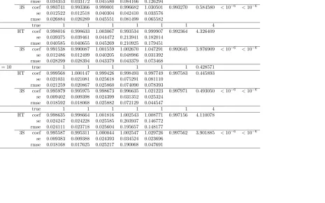
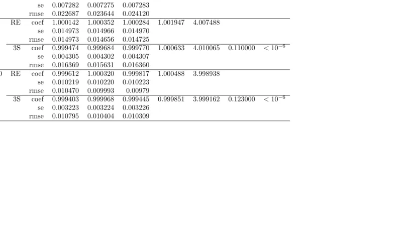
For the Hausman-Taylor world, we compare the IV method proposed by Hausman and Taylor (1981) with our robust 3S estimator. Table 4 gives the results for N = 100,
T = (5,10),ε= 0.5 andρ= 0.3,0.8. It shows very good estimates of the slope coefficients with 3S, except for η2 which is slightly biased. The coefficient β2 of the time-varying
variablex2,(correlated withµi), is also well estimated. Similarly, the coefficientη1 of the
time-invariant variableZ1,(uncorrelated withµi), is also well estimated. In contrast, the
coefficientη2 of the time-invariant variableZ2,(correlated with µi), is slightly biased (3%
to 4.7% for (N = 100, T = 5) and 2.1% to 2.9% for (N = 100, T = 10)). This bias does not change when N increases (see Table A8 in the Appendix). However, the standard errors are considerably lower, especially for the coefficients η1 and η2 of the two
time-invariant variables. The 95% confidence intervals obtained with 3S are much narrower and are entirely nested within those obtained with the IV procedure of Hausman-Taylor. For instance, from Table 4, the average over 1,000 replications of the 95% confidence intervals forη2 are:
95% confidence intervals forη2 3S IV HT
min max min max
N = 100, T = 5 ρ= 0.3 0.965 1.096 0.740 1.249
ρ= 0.8 0.984 1.107 0.643 1.356
N = 100, T = 10 ρ= 0.3 0.971 1.070 0.838 1.156
ρ= 0.8 0.983 1.076 0.721 1.296
The HT procedure is known to generate large confidence intervals for all the coefficients of the time-invariant variables. Despite the fact that our 3S method leads to a slight bias for the coefficientη2of the time-invariant variableZ2 (correlated withµi), the uncertainty
While the biases are similar to those of HT, the RMSE are much smaller (for instance, the RMSE of η2 is three times smaller when N = 100,T = 10 and ρ= 0.8). Whereas 3S
and HT fit the remainder variance rather well (σ2ε), 3S tends to slightly over-estimate the individual effects variance (σ2
µ) when ρ is small, and under-estimate it whenρ is large.
When ρ= 0.3, the bias of σµ2 for HT declines from 17.05% to 4.57% when T doubles. The comparable decline for 3S is from 36.40% to 15.04% whenTdoubles. This bias shrinks considerably whenρ= 0.8.In fact, for HT, there is a reduction in the bias from 8.16% to 2.75% when T doubles. The comparable reduction in the bias for 3S is from −0.57% to 2.49%. These results continue to hold when N increases (see Table A8 in the Appendix). Just like the Mundlak and Chamberlain-type FE worlds, the weightsλβandλbindicate
that there is no trade-off between the Bayes estimators and the empirical Bayes estimators. Only the empirical Bayes estimators are used in the estimation of the slope coefficients and the individual effects. For a typical macro-panel (N small,T large), all these results carry through, and in some cases are even improved (see Table A9 in the Appendix forN = 50,
T = 20, ρ = 0.8 with ε = 0.5). We see that the bias on the coefficient η2 of the
time-invariant variable Z2 (correlated with µi) is reduced to 1.5%,and more importantly the
standard errors are 8 times smaller than those obtained for the IV procedure of Hausman-Taylor. Once again the 95% confidence interval for η2 obtained with 3S [0.966; 1.065] is
smaller and nested within that obtained for the HT estimator [0.606; 1.397]. Moreover, the bias ofσµ2 for HT is larger (3.06%) than that for 3S (−0.52%).
To investigate the properties of our proposed strategy, we computed the biases (η2−
bη2,3S) under s = 1,2,3. Figures 1 and 2 in the Appendix plot the ratios of the biases fors = 2,3 relative to the bias for s= 1 for different sample sizes. The figures confirm that when the correlation betweenµi and Z2i is more than 20%, it is best to uses= 1 to
reduce the bias. Whereas when the correlation betweenµi and Z2i is less than 20%, it is
best to uses= 2,3 to reduce the bias.
5.3 Sensitivity to ε and non-normality
As a final check on the properties of our proposed 3S estimator, we conducted two ad-ditional sets of experiments. First, we checked the sensitivity of our results to changing the values of ε, the contamination part of prior distributions. We allowed ε to vary be-tween 10% and 90%. Only the results for the RE world and the Hausman-Taylor world (N = 100, T = 5, ρ= 0.8) are reported in Tables A10 and A11 in the Appendix. For the RE and HT worlds, this does not change the estimated slope coefficients, standard errors, biases or RMSE of the coefficients. It also does not change the estimated values of the remainder variances (σε2). Only for HT do we observe some differences in the variances of the individual effects (σµ2). The closer we are to the intermediate values (ε= 0.3,0.7), the more important is the bias (−2.5%). For extreme values (ε= 0.1 or 0.9), the bias is smaller (−1.75%). For ε= 0.5, we get the smallest bias (−0.75%). Moving from ε= 0.1 toε= 0.9 leads to a W shape for the bias onσµ2.
Last, but not least, we checked the sensitivity of various estimators to a non-normal framework. The remainder disturbances (εit) were assumed to follow a right-skewed t
-distribution ST(0, df = 3, shape = 2) (see Fern´andez and Steel (1998)) instead of the
N(0,1) (see equation (53)). Results in Tables A12-A14 in the Appendix show that, irre-spective of the estimator considered, our 3S significantly dominates in terms of bias and precision of the slope parameters for RE, Chamberlain-type fixed effects and Hausman-Taylor worlds. In addition, the estimated variances of the individual effects and remainder terms are much closer to the true theoretical values compared to the classical estimators. What is remarkable is that our 3S estimator remains unbiased and has very small standard errors relative to the classic estimators. It also yields variances of the individual effects
σ2
for the Hausman-Taylor world, Table A14 in the Appendix shows that the bias of our 3S estimator for η2 is −0.38%, while that for HT is 1.02%. But most surprising, the 95%
confidence interval ofη2 is very narrow [0.8447; 1.1628] as compared to the wide 95%
confi-dence interval [0.3035; 1.6761] for HT. The estimates ofσ2
ε of our 3S estimator (7.221) and
the HT estimator (7.211) are close to the theoretical variance σε2= 7.227. However, this is not the case for the estimated individual effects varianceσ2µ.Our 3S estimator (4.571) is relatively closer to the theoretical value (σ2
µ= 4) as compared to that of HT estimator
(5.558). Last but not least, λβ is small but slightly more important than that for the
Gaussian cases.
6
Applications
6.1 The Cornwell-Rupert earnings equations
Cornwell and Rupert (1988) estimate a returns to schooling example based on a panel of 595 individuals observed over the period 1976−82 and drawn from the Panel Study of Income Dynamics (PSID). In particular, log wage is regressed on years of education (ED), weeks worked (WKS), years of full-time work experience (EXP), occupation (OCC=1, if the individual is in a blue-collar occupation), residence (SOUTH = 1, SMSA = 1, if the individual resides in the South, or in a standard metropolitan statistical area), industry (IND = 1, if the individual works in a manufacturing industry), marital status (MS = 1, if the individual is married), sex and race (FEM = 1, BLK = 1, if the individual is female or black), union coverage (UNION = 1, if the individual’s wage is set by a union contract) (see also Baltagi and Khanti-Akom (1990)). We letX1 = (OCC, SOU T H, SM SA, IN D),
X2 = (EXP, EXP2, W KS, M S, U N ION), Z1 = (F EM, BLK) and Z2 =ED. For the Mundlak estimation, we drop Z1 and Z2 and we consider that only the variables in X2 are correlated with the individual effects.
The estimation results are reported in Table 5. There are very few differences between the Within, the FGLS estimates on the transformed model (i.e., the Mundlak-type FE) and our 3S estimator. Since we assume that only the X2 variables are correlated with the individual effects, Within estimates do not exactly match the Mundlak-type FE. One can note that the FE estimates are slightly different from those of the two other methods (Mundlak-type FE and 3S), especially forOCC, SOU T H and SM SA. But for the main variables of the earnings equation, we get similar results. A comparison between the Mundlak-type FE and 3S shows that the estimate ofIN D becomes significantly different from zero. With the three-stage robust Bayesian estimator, we get more precise estimates of all coefficients. Estimation of theπvalues from the 3S and the FGLS on the transformed model are quite similar. The estimated variances of the individual effects (σµ2) and the residuals (σ2
ε) are roughly the same for 3S and Mundlak-type fixed effects.
For the HT model, we need to reintroduce Z1 andZ2 into the model. The assump-tion that there is correlaassump-tion between the individual effects and the explanatory vari-ables X2 and Z2 justifies the use of the IV method with instruments given by AHT =
[QXX1, QWX2, P X1, Z1] whereQW =IN T−P is the within-transform. To choose thes
parameter of our functionf[.] = (x2,i−Ex2)
2⊙(Z
2i−EZ2)
s, we estimate the OLS proxy
of the individual effects bµ = Z′
µZµ−1Zµ′ybwhere by are the fitted values of the pooling
regression y = X1β1+ X2β2 +Z1η1+Z2η and then compute the correlation between µb
and Z2. The estimated correlation is large (0.612), so we set s = 1. From the estimates
forSM SA. With the IV method, we get non significant effects for OCC, SOU T H and
IN D and a surprising negative effect for SM SA. In contrast, with the 3S estimator,
OCC and SOU T H have the expected negative effects. IN D has an expected positive effect but SM SA has a non significant effect. With 3S, gender and race effects are now significant and the plausible negative gender impact dominates the negative race effect. If EXP and EXP2 have the same impact in both the 3S and HT, the effect of ED is slightly lower (11.43% against 13.79%).13 More interestingly, the 95% confidence interval
of ED is narrow [11.02%; 11.83%] as compared to the one obtained with the IV method [9.63%; 17.56%]. This sizeable difference between the standard errors of 3S and those of the IV method are expected from our Monte Carlo study. However, there is no statistical difference between these two estimates, since the confidence interval of ED for IV nests the one for 3S. From an economic policy point of view, though, the effect of education on earnings is better estimated with 3S than with IV. It is difficult to imagine an economic adviser telling a policy-maker that the returns to schooling effects can vary between 9% and 17%. Yet, one may wonder whether the average education effect estimated with 3S may be under-estimated, the difference being less than 2.4%.14
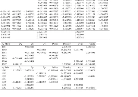
6.2 The Cornwell-Trumbull crime model
Cornwell and Trumbull (1994) estimated an economic model of crime using panel data on 90 counties in North Carolina over the period 1981−1987. The empirical model relates the crime rate to a set of explanatory variables which include deterrent variables as well as variables measuring returns to legal opportunities. All variables are in logs except for the regional dummies (west,central). The explanatory variables include the probability of arrest PA , the probability of conviction given arrest PC, the probability of a prison
sentence given a conviction PP, the number of policemen per capita as a measure of
the county’s ability to detect crime (P olice), the population density, (Density), percent minority (pctmin), regional dummies for western and central counties. Opportunities in the legal sector are captured by the average weekly wage in the county by industry. These industries are: transportation, utilities and communication (wtuc); manufacturing (wmf g).
From Table 7, there is not much difference between the MCS and 3S estimates on the transformed model.15 All the confidence intervals for MCS and 3S estimates overlap.
Estimation of theπtcoefficients obtained from 3S lead to more statistically significant
co-efficients than those from MCS. We only report coco-efficients that are statistically significant at the 5% level. But, more interestingly, we note a strong coherency between the Within estimates (FE) and 3S. The MCS estimates are slightly different from the FE estimates, with, for example, PC having an estimate of −0.23 for MCS as compared to −0.31 for
FE and 3S. Note, however, that the 95% confidence intervals overlap with each other. The estimated variances of the individual effects (σµ2) and the residuals (σε2) are sighltly different (0.05 for 3S and 0.07 for MCS).
We also estimated a Mundlak-type FE model. Table 8 reveals slight differences between the Within, the Mundlak-type and 3S estimation results. The most notable differences concern the dummies, the π values and the standard errors between 3S and Mundlak-type FE. Estimation of all the coefficients by 3S are more precise than those of the FGLS
13
Baltagi and Bresson (2012), using a robust HT estimator, show that the returns to education are roughly the same but the gender effect becomes significant and the race effect becomes smaller as compared to those obtained in the classical HT case.
14Recall that the coefficient of the endogeneous time-invariant variable was slightly biased (1
.7% to 5%) in the simulation study for 3S, even though the RMSE for 3S, was lower than that for HT.
15
Results are obtained using one hundred iterations on the MCS estimator to match the results of Baltagi