Research on Location Routing Problem (LRP) Based on Chaos Search (CS) and Empirical Analysis

(1)

Research on Location Routing Problem (LRP) Based on

Chaos Search (CS) and Empirical Analysis

Qian Zhang1, Zhongming Shen1, Xianji Zhang2

1_{School of Economics and Finance, HuaQiao University, Quanzhou, China} 2_{BPS Global Group, Hong Kong, China}

Email: [email protected], [email protected]

Received November 21, 2012; revised December 22, 2012; accepted January 8,2013

ABSTRACT

Due to the problem complexity, simultaneous solution methods are limited. A hybrid algorithm is emphatically proposed for LRP. First, the customers are classified by clustering analysis with preference-fitting rules. Second, a chaos search (CS) algorithm for the optimal routes of LRP scheduling is presented in this paper. For the ergodicity and randomness of chaotic sequence, this CS architecture makes it possible to search the solution space easily, thus producing optimal solutions without local optimization. A case study using computer simulation showed that the CS system is simple and effective, which achieves significant improvement compared to a recent LRP with nonlinear constrained optimization solution. Lastly the pratical anlysis is presented relationship with regional logistics and its development in Fujian province.

Keywords: Clustering Analysis; Chaos; Chaotic Behavior; Location Routing Problem (LRP);Logistics Distribution;

Optimization; Regional Logistics

1. Introduction

All companies that aim to be competitive on the market have to pay attention to their organization related to the entire supply chain. In particular, companies have to in- crease the efficiency of their logistics operation. It is es- sential that reasonable optimal systems of logistics distribution for enterprises with the development of e-com- merce and integrated logistics. Location-routing problem (LRP) is an important branch of routing optimization in integrated logistics systems, which has been solving for every logistics distribution corporations.

The conceptual foundation of LRP studies dates back to Von Boventer (1961), Maranzana (1965), Webb (1968), Lawrence and Pengilly (1969), Christofids and Eilon (1969) and Higgins (1972) [1]. Although these earlier studies are far from capturing the total complexity of LRP, they first recognized the close interface between location and transportation decisions. Watson-Gandy and Dohrn（1973）may be some of the first authors credited to consider the multiple-drop nature of the vehicle routes within the location-transportation framework [2]. Many scholars have developed more efficient problem solving techniques using the concept of integrated logistic systems, which include optimal models and their algorithms. Due to its complexity, it is models and algorithms that are core for solving LRP, which is NP-hard. More and more scientists have been interested in these works. Ex-

act algorithms and heuristics are given in some articles. Exact algorithms for LRP can be classified into four cate- gories: direct tree search (branch-and-bound), dynamic programing, integer programming, and non-linear programming. Heuristic includes location-allocation-first, route-second, route-first, and location-allocation-second, savings/insertion, and improve/exchange [3].

Chaotic system is a common phenomenon exiting in nonlinear dynamical system with popular characteristic of dynamics. Due to the ergodicity and randomness of chaotic sequence, the chaos search (CS) architecture can be solved the traditional optimization [4]. Much of engineering is concerned with the topic of optimization, and at the heart of much of the optimization are dynamical systems. Dynamical systems can be thought of either nonlinear continuous-time differential equation. Chaos occurs in dynamical systems, and frequently in engineering, which becomes the central fascination. Some of domestic scholars use chaos search for nonlinear optimi-zation with constraints. The main advantage is to search the solution in certain field regardless of the continuous and difference of the function that can be solved complex optimization with constrains. Furthermore, it is easy to seek the optimal solutions (or near optimal solutions) without local optimization.

(2)

chaos search, together with a proof of their correctness [5]. Several clusters are divided by preference-fitting rules. Then the optimal route has been found using chaos in every cluster [6]. The simulation results show that it is an effective method. The paper is organized as follows.

Section 2 introduces the meaning and descriptions of LRP and describes the mathematical model of LRP. Sec- tion 3 emphasizes on the hybrid algorithm based on clustering analysis and chaos search for LRP. Section 4 shows the computational results and analysis. Finally, the last section gives conclusions and future work.

2. Description of LRP

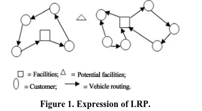
Location-routing problem (LRP) is one of the problems in integrated logistics optimizations. The LRP can be defined as follows. A feasible set of potential facility sites and location; and expected demands of each customer are given. Each customer is to be assigned to a facility, which will supply its demand. The shipments of customer demand are carried out by vehicles, which are dispatched from the facilities and operated on routes that include multiple customers. There is a fixed cost associated with opening a facility at each potential site, and a distribution cost associated with any routing of vehicles that includes the cost of acquiring the vehicles used in the routing, and the cost of delivery operations. The cost of delivery operations is linear in the total distance traveled by the vehicles [7]. The LRP is used to determine the location of the facilities and the vehicle routes from the facilities to customers, with the aim of minimizing the sum of the location and distribution costs, while ensuring that the vehicle capacities are not ex- ceeded [8]. The expression of LRP is given in Figure 1.

A constraint-based model is presented in this paper for the location routing problem. The hypotheses are as follows:

The transportation is just in time.

The facility is both starting point and destination of circular vehicle routing; each facility serves more than two customers.

[image:2.595.76.280.607.719.2]

Nature of demand/supply: deterministic.1 There are multiple facilities.

Figure 1. Expression of LRP.

Size of vehicle fleets: single vehicle (A facility is served by one vehicle; meanwhile, it is satisfied that the total demand of the route is no less than one vehicle’s capacity).

Vehicle capacities are determined. The total quantity (amount) of goods is limited in every route by each vehicle’s capability.

Facility capacities are undetermined; not all facilities have been chosen in every decision.

Each customer is served by one and only one vehicle. Considering the complexity of supply/demand markets, it is assumed that they are retail markets.

Each facility is considered a separate entity, not linked to the other facilities.

Objective: minimize total costs.

2.1. Decision Variables Considered Are as Follows

1,if vehicle goes from customer to customer

, , , , ,

0, otherwise

1,if a facility is establishe atsite , 0, otherwise

ijk

r

k i

x j i S j S k V i j

d r r G

Z

 

_    

 

 

  

2.2. Model Parameters Are Given as Follows



1, ,



G r r  m

is the set of m feasible sites of candidate facility,



1 ,



H i i m  , m N

is the set of N customers to be served,

   

S G  H

is the set of all feasible sites and customers (it is also referred to nodes),



k 1, ,



V v k  K

ij

C

node to node ,i j i S j S ,  ,

is the set of K vehicles available for routing from the facilities, average annual cost per distance traveling from

r

F annual cost of establishing and operating a facility at site r r



1, , m



, q_j average number of units demands by customer j j H







, Q_k capacity of vehi- clek k



1, , K



, d_ij

,

rik rjk

distance from node i to node j,

X X

The objective function of LRP is

traveling by vehicle k from node r to customer

i or to customer j, respectively.

2.3. Model of a Special LRP Is Defined as Follows

(3)

 

min ij ijk ij r r r G i S j S k V

f x 

 

C X d F Z







(1)

Subject to

1, ,

  

ijk k V i S

X   j H (2)

, ,

k

Q k V

   (3)

, ,

 

 

j ijk i H j S

q X

 

 

0,ipk pjk

i S j S

X X  k V p S (4)

,

 

1,

 



G rjk

r j H

X   k V (5)

1, , , ,

 

2, rjk r j

 

k V

X Z Z 



 m  R r G (6)

0, ,



rik r k V j H

X Z  r G (7)

, ,

 

 

 

0,

rik r j H

X Z  k V r G (8)

, , ,



 



0 or 1,

ijk

X i j S k V  (9)

.

 

0 or 1

r

Z r G unctio ta

orithm Based on Clustering

3.1

r techniques in pat-

 

In this model, the objective f

(10) n minimizes the to- l cost of routing, and establishing and operating the facilities. Constraint (2) ensures that each customer is served by one and only one vehicle. Constraint (3) ensures that the vehicle capacity constraints are not ex- ceeded for any of the vehicles used in routing, while (4) is the route continuity constraint, which implies that the same vehicle should leave every point that is entered by a vehicle. Constraint (5) guarantees that each vehicle is routed from one depot. Constraint (6) guarantees that there are no links between any two depots. Constraints (7) and (8) require that a vehicle can only from a depot if that depot is opened. The last two of constraints are the integer constraints.

3. A Hybrid Alg

Analysis and Chaos Search for LRP

. Clustering Analysis of LRP Clustering analysis is one of the majo

tern recognition. It is a technique for grouping data and finding where similar data are assigned to the same cluster whereas dissimilar data should belong to different clusters. The conventional clustering methods generate partitions, in a partition; each pattern belongs to one and only one cluster.

The customer aggregate C is divided to cluster by the euclidean measure. The steps of optimal facility location are performed in the following way, which have exten- sively analyzed and used in location theory to approxi- mate distances between two spatial coordinates. For the sake of simplicity, it is assumed that each facility has its

own set m of their coordinates of candidate sites for facility location, and no two facilities share the same location, which are denoted by

















1 1 1 2 2, 2 , ,

, , , , .

i i i m m m

F X Y PF X Y PF X Y

 

Every two coordinates of candidates sites for facility

lo i i

, ,

PF X Y P

cations are denoted by PF X Yi



,



and PF X Yj



j, j



,

and which satisfied with



 



1 2

ij i j i j

R1 2 X _X 2_ Y Y_ 2

 

  (11)

where Rij is one half of the distance between



,



i i

PF X Yi and PF X Y . j



j, j



given as

Rules for classification are follows.

(12)

Ｃp can only be divided if form

fe

max

Rule1 rip Rij

into PFi ula (12) is true.

Rule 2 The coordinates of customers on the circum-

rences are satisfied that the distance to the nearest two customers is less than that to the sub nearest two points. sub-nearest meaning that they are not included a cluster by reason of distance).

Rule 3 If jq  ij (13)

whe jq any custom

e numbers of customers,

r R

re r is the distance from er Cq to any facility PFj, maxRij is half of the most distance between

any two facilities. Either these customers will not be served, or else the candidate’s facility location will be abolished. Last two rules only relate to abnormal customers points.

where Ｎ is th

















1 1 , , , , , ,

N

p p p N N N

C x y C x y



１２１

are expressed the points and their coordinates, respec-

the distance between any candidate facility PF

an

3.2. An Algorithm of Chaos Search Optimization

The l idea is that chaotic sequences belonging , , , , ,

C C C C C x y

tively.

rip is i

d any customer p. The tangent cycles O1, O2, …, Oi,

Oj, …, Om are drawn with the radius Rij, where R1, R2, …,

Ri, Rj, …, Rm are their radiuses, respectively.

for LRP

fundamenta

(4)



1

: k k 1 k



f x    x x (14)

where  is the so called driving param g

eter(a parameter capturin such factors as fertility rate) initial living area, etc. The initial value, or seed x is in

 

0,1 .



 



2,4





, There f

   

0,1  0,1 if 0  4.From

restricted

about x is to

 

0,1 and to

 

The characteristic of ogistic map is given as follow: 0, 4 .

L

1) When λ to

 

2,3 , there are stable points in Logis- tic map.

2) When λ to



3,3.57



erge ve

t in stabl

that is

, two sequences with seeds only slightly apart div ry rapidly, that is to say, there exists in the period-doubling bifurcation of the solutions.

3) When λto



3.57, 4



, chaos start to come out, and Logistic map isn’ e cycling orbit. It is difficult to decide which points with Lebesgueis more than zero in chaotic sequences.

4) When λto 4, there is a stable chaotic sequence. In the stable chaotic sequence, any orbit f is dense, to say, the points of one orbit f is included in open ball

 

,

B x , when   0, and x

 

0,1 . On the con- trary, all points that belong to



0,1



are

s po

pressed on towards any orbit f as precision a ssible. In this paper when  4, the population sequence

 

Xk is chaotic and erg and gives search optimal solutions (or near optimal solutions) solutions. A chaotic system is defined as one where two different, but close, seeds result in widely different population sequences. An ergodic system is one where the sequences

 

k

odic

X will approach every possible point arbitrarily, littl y little (more for- mally, for every pair of element of



e b



0,1 , there is an xk

between them). Thus, an ergodic sy is one that is “trying to converge to everything”. The Logistic model can be solved not only for the continuous variable optimization, but also discrete variable optimization.

3.3. A Hybrid Algorithm for LRP stem

ps. First, prefer-



1



1 , r

i i d C C 



(15)

where

The hybrid algorithm includes two ste

ence-fitting rules to solve location-allocation cluster the customers. Second, the optimal routes is obtained by chaos search to be minimized the function. The Logistic chaotic model is transformed for discrete optimization of LRP [11]. A legal route will be determined with the numbers customer of r in one cluster, that is to say, the order of the customer clusters will be arranged [12]. The variable d indicates the route distance in any cluster to be minimized.

min i





1 1, , 1

i d C Ci i (16)

denoted the distance betwe custom C C

en er C_i and cus-

tomer Ci1.

Steps with the hybrid algorithm based on clustering an

fitting ru

itial calculations for Rij and rip are performed. i.

alysis and chaos search are described as follow. Step 1 Customers are clustered by preference-les.

1) In

2) If rip<Rij, the customer p is divided into cluster O

3) Otherwise, return step (1.1).

Step 2 X i i

 

1, 2, , r



is given by initial random value. The best optimal value of the function opt f_ 0, given with the control parameter k gifted wi r value.

Step

th a large

3 Put the results of order arranged X

 

i into

 

i . It is obtainable to a current searching route, and to rent legal route by hybrid algorithm, compared with Y

a cur

   

, X i Y i .

Step 4 Calculate the function values f of the current le

emember the minimum function values gal route.

Step 5 R

_ : _ ,

pt f f opt f

o  and opt f_  f, step 0, and also resent

Step 6 Decide whether the cycle is remembering the p legal route.

stopped or not. If st

f ep = k, stop.

Step 7 A set o X

 

1,m is generated by Logistic map, st

teps 3, and cycling.

4. Analysis of the Computational Results

and

ulation results are shown in Table 2. As seen

in

5. Empirical Analysis

iven in relationship between ep = step + 1.

Step 8 Return s

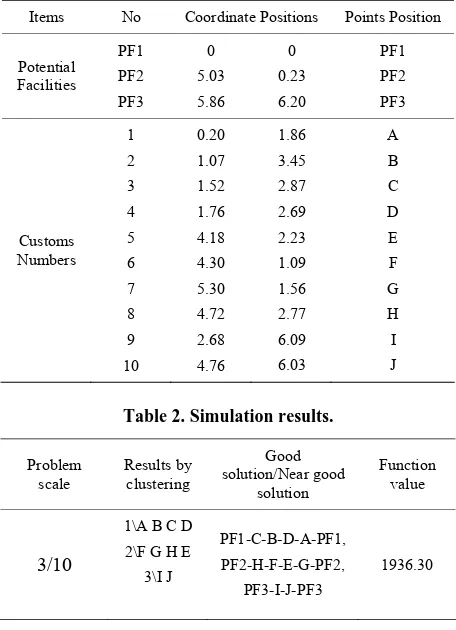
In the following example three potential facilities, ten customs were analyzed. Each was served. With the same type of distribution vehicle that had a carrying capacity equal to 30 ton. The annual cost establishing and operating a facility Fr is equal to 160 yuan/each, The

transportation cost Cij is equal to 2 yuan per ton, per km.

The hybrid algorithm has been discussed to search the optimal route based on the data in Table 1.The pro-

gramming is edited by VC++. The results of clustering analysis and running by 50,000 times are given in Table 2.

The sim

this table, it is an effective method based on clustering analysis and chaos search proposed in this paper. This method can be sought optimal solution (or near optimal solutions) adaptively and quickly for many candidate facilities and customers. Thecomputational cost is dramatically reduced by chaos search to solving the small- scale question. The proposed optimal algorithm provides a new path for large-scale optimization in practical integrated logistics

The empirical analysis is g

(5)

Table 1. Coordinate position of three potential facilities and ten customs.

Items No Coordinate Positions Points Position

Potential _5. _0.

Facilities

PF1 PF2 PF3

0 0

03 5.86

23 6.20

PF1 PF2 PF3

Customs Numbers

1 2 3 4 5 6 7 8 9 10

0.20 1.07 1.52 1.76 4.18 4.30 5.30 4.72 2.68 4.76

1.86 3.45 2.87 2.69 2.23 1.09 1.56 2.77 6.09 6.03

[image:5.595.309.535.82.281.2]

A B C D E F G H I J

[image:5.595.58.286.112.427.2]

Figure 2. The trend of each variable.

Table 3. ADF unit root test results of each variable.

Test type ADF Test _{5% level} _{10% level}

Table 2. Simulation results.

Problem Results by _solutio _ood Function scale clustering

Good n/Near g

solution value

3/10

1\A B C D

PF1-C-B-D-A-PF1,

1936.30 2\F G H E

3\I J PF2-H-F-E-G-PF2, PF3-I-J-PF3

ith analysis is proposed for the relationship with mod-

5.1. Unit Root Test

e letters of C, T, K means inter-

tim

5.2. Co-integration Test

test is accepted for GDP,

Table 4, refused to no co-integration variables

of w

ern logistics and GDP. The factors are chosen include GDP, logistics production value (WLCZ), freight turnover (HZL), logistics mileage (WLC), and which the data is chosen from 1978 to 2010. The unchangeable price in1978 is given with each variable. The quantitative software is accepted with EVIEWS 6.0, and which the trend of each variable is give in Figure 2 including GDP,

WLCZ, HZL,WLC.

Test type (C, T, K), Th

cept, Trend, lagging numbers. The first four are contains intercept and trend; The after four are not contains trend.

From the Table 3, it is known that the original data in

e trend, after an order difference or second order difference, the data is smooth.

The Johansen co-integration

WLCZ, HZL, WLC. This test results is presented in Ta- ble 4.

From

the null hypothesis in 5% level of trace statistics.

(C, T, K) statistic

GDP (C, T, 1) 3.28 –3.56 –3.21 WLCZ (C, T, 1) –1.11 –3.55 –3.21 HZL (C, T, 1) 2.14 –3.55 –3.21 WLC (C, T, 1) –0.28 –3.55 –3.21 D2_GDP _{(C, T, 1)} _–4.45 _–3.57 _–3.22

[image:5.595.309.537.309.474.2]

DWLCZ (C, T, 8) –5.58 –3.56 –3.21 DHZL (C, T, 8) –4.96 –3.56 –3.21 D2_WLC _{(C, T, 8)} _–6.65 _–3.59 _–3.23

Table 4 Johansen test results.

Null hypothesis Trace statistic 5% level Eigenvalue

r = 0*_52.09_47.85_0.58

r≤ 1 2.85 29.79 0.41

r≤ 2 18.14 15.49 0.23

r≤ 3 0.04 3.84 0.001

Note: Th rs of r means ers of co-i ion equa eans

his demonstrates that the variable is at least one co-

DP 1.784WLCZ 1.364WLC 1.91HZL

e lette numb ntegrat tion, *_m

reject null hypothesis.

T

integration equation between the relationships, that there is a long-term equilibrium relationship between variables.

G    

(2.22) (0.88) (0.24) )

ru

[image:5.595.313.537.500.587.2]

(6)

HZL ECMt 1

 

 

(3.01) (6.84)

18)

From the equation, T statistics test of al si

W

6. Conclusions

r, it has been proposed that the

effec-rial optimization

7. Acknowledgments

part by National Natural

REFERENCES

[1] J. H. Bookbi “Vehicle Routing

between variables. Therefore, it is necessary to establish Science Foundation of China under grant number 71040009, in part by Program for New Century Excellent Talents in University under grant number NCET-10- 0118, in part by Youth Foundation of Chinese Education by HuoYing-dong under grant number 104009.

the error correction model (ECM), to estimate short-term changes between variables. Estimated ECM is give as following:

GDP 4.141 WLCZ 0.498 0.846 WLC 0.472

   

   

(1.90) (–2.58) (

AdjustedRsquared 0.747 Considerations in Distribution System Design,” nder and K. E. Reece, European Journal of Operation Research, Vol. 37, No. 2, 1988, pp. 204-213. doi:10.1016/0377-2217(88)90330-X

[2] D. B. Bruno, F. Vincent, S. Paul, K. Philip an l variables are

gnificant in level 10%, the error correction of ECMt-1 coefficient is negative, accord with reverse revision mechanism, thus further shows that the error correction model is good, with residual sequence is the white noise.

By comparing the co-integration equation and ECM,

d P. Pat- rick, “Solving Vehicle Routing Problems Using Constr- aint Programming and Metaheuristics,” Journal of Heu- ristics, Vol. 6, No. 4, 2000, pp. 501-523.

doi:10.1023/A:1009621410177 [3] V. Campos and E. Mota, “Heu e can conclusion that t compared on short-term, freight

turnover (HZL) have negative influence on the GDP in long term, but its elasticity coefficient is greater than the short-term elastic coefficient; Output value of logistics (WLCZ) have short-term elastic significantly greater than its long-term flexibility to GDP, and both have different symbols, changes of direction that does not accor- dance, it indicates that in recent years the logistics infra- structure investment lead to the logistics industry close to a saturation stage in Fujian province, although output value of logistics (WLCZ) promote the growth of GDP in short-term, but due to the expansion of the regular, the GDP growth plays a role of obstacles in the long term.

ristic Procedures for the Capacitated Vehicle Routing Problem,” Computational Optimization and Applications, Vol. 16, No. 3, 2000, pp. 265-277. doi:10.1023/A:1008768313174

[4] L. Cooper, “The Transportation-Location Problem,” Op- erations Research, Vol. 20, No. 1, 1972, pp. 94-108. doi:10.1287/opre.20.1.94

[5] G. Dijin, “Hybrid Evolutionary Method for Capacitated

in In-

Design of Supply-Chain Logistics Sys- Location-Allocation Problem,” Computer and Industrial Engineering, Vol. 33, No. 3-4, 1997, pp. 577-580. [6] V. Fernando and A. Joaquin, “Homoclinic Chaos

verted Pendula,” Proceeding of the 39th IEEE Conference On Decision and Control, Sydney, 12-15 December 2000, pp. 4821-4822.

[7] H. Heung-Suk, “

tem considering Service Level,” Computers and Indus- trial Engineering, Vol. 43, No. 7, 2002, pp. 283-297. doi:10.1016/S0360-8352(02)00075-X

[8] G. Laporte, “Hamiltonian Location Pro In this present pape

tive method for LRP using a hybrid algorithm based on clustering analysis and chaos search. Through computer simulations the method has been shown to solve large- scale LRP. Using the clustering technique, the computational cost is dramatically reduced. Due to the feature of chaotic global ergodicity, the optimal routes are random- ly seeked in one cluster, which ensures search efficiently and produces optimal solutions (or near optimal solutions) without local optimization. Thus, the emphasis is directed towards developing a methodology, which has been improved the quality of solution.

The application to other combinato

blems,” European Journal of Operation Research, Vol. 12, No. 1, 1983, pp. 80-87. doi:10.1016/0377-2217(83)90182-0

[9] G. Laporte and Y. Nobert, “An Exact Algorithm for Minimizing Routing and Operating Costs in Depot Loca- tion,” European Journal of Operation Research, Vol. 6, No. 2, 1986, pp. 224-226.

doi:10.1016/0377-2217(81)90212-5

[10] J. Ra, “Dissipative Enterprises, Chaos, and the Principles

Gandy and P. Dohrn, “Depot Location with of Lean Organizations,” Omega, Vol. 26, No. 6, 1998, pp. 397-340.

[11] C.

Watson-van Salesmen—A Practical Approach,” Omega, Vol. 1, No. 3, 1973, pp. 321-329.

doi:10.1016/0305-0483(73)90108-4 [12] P. N. William and J. B. Wesley, “So problems should be investigated in integrated logistics.

The relationship is given with regional logistics and its development. There exists a long-term equilibrium rela- tion between economics growth and logistics development in Fujian province.

lving the Pickup and

9)00016-8

Delivery Problem with Time Windows Using Reactive Tabu Search,” Transportation Research Part B, Vol. 34, No. 2, 2000, pp. 107-121.

doi:10.1016/S0191-2615(9