Employing Gene Expression Programming in Estimating
Software Effort
Najla Akram AL-Saati,
PhD
Assist. Professor, Software Engineering Dept.
College of Computer Sciences & Mathematics,
University of Mosul, Iraq
Taghreed Riyadh AL_Reffaee
Assist. Lecturer, Software Engineering Dept.
College of Computer Sciences & Mathematics,
University of Mosul, Iraq
ABSTRACT
The problem of estimating the effort for software packages is one of the most significant challenges encountering software designers. The precision in estimating the effort or cost can have a huge impact on software development. Various methods have been investigated in order to discover good enough solutions to this problem; lately evolutionary intelligent techniques are explored like Genetic Algorithms, Genetic Programming, Neural Networks, and Swarm Intelligence. In this work, Gene Expression Programming (GEP) is investigated to show its efficiency in acquiring equations that best estimates software effort. Datasets employed are taken from previous projects. The comparisons of learning and testing results are carried out with COCOMO, Analogy, GP and four types of Neural Networks, all show that GEP outperforms all these methods in discovering effective functions for the estimation with robustness and efficiency.
Keywords
Effort Estimation, Software Engineering, Artificial Intelligence, Gene Expression Programming.
1.
INTRODUCTION
Administration and organization of Software projects usually starts with planning, any project cannot be initiated before an estimation of the work to be done, the essential resources, and the time necessary to complete the project is carried out by the development team.[1]
It is very crucial to provide good estimates of the effort and cost required in completing projects during the inception phase.[2] After doing so, a schedule should be prepared by the development team describing software engineering responsibilities and milestones, it should also decide who is in charge of accomplishing such tasks[1].
Common problems related to the process of estimation are associated with overestimation or underestimation of the desired effort. Underestimation can cause low self-confidence for employees, weakening in reputation and a demanding work situation. In contrast, overestimation can produce a situation where a lot of resources are bound to the project, or produce inadequate decisions concerning outsourcing project parts, as opposed to constructing it internally. By and large, software industries tend to underestimate the effort, which can lead to accepting that milestones can’t be met during execution [2].
Software has lately become the highest costly part of a project; hence the impact of worthy estimation in a software project is essential. A lot of estimation models were introduced over the last 4 decades and they were all confronted with the same problem: when the software size and significance increase it becomes more complex, then the accurate prediction of effort or cost can be very difficult.
However due to the high-speed varying nature of software development, it is becoming very hard to develop models that provide high accuracy for software development in all areas. The estimation process usually involve finding Effort (Person-months), Project Duration (Calendar time), and/or Cost (Dollars) [2].
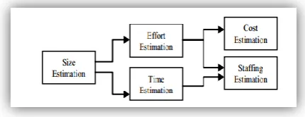
Figure 1 shows the sequence of estimates in the life cycle of the Software development. [3]
Fig 1: Sequence of Estimation in System Development Life Cycle [3]
There has been a vast work presented for software effort estimation starting from traditional and mathematical approachessuch as COCOMO and Function Point Analysis. These methods do not regularly yield accurate cost or effort estimates. Lately, Artificial Intelligent methods began to attract more interest, they have been intensively investigated in the literature. This work focuses on employing Gene Expression Programming to find suitable estimates for software effort.
2.
LITERATURE REVIEW
[image:1.595.323.539.304.387.2]and ISBSG were used to validate the model. He employed 3-Fold cross validation for evaluating the accuracy of predictions for different models.[11]Whereas Ziauddin, Tipu, and Zia in 2012, developed an effort estimation model for of Agile Software by employing traditional methods and 21 projects. [12] Toka and Turetken proposed a comparative analysis for the accuracy of models of contemporary parametric software estimation.[13] In the same year, Israa [14] proposed an analysis of the performance for neural networks, the results were compared with the COCOMO model
Arnuphaptrairong proposed in 2013 a Function Point methodology along with a data flow diagram to perform estimation in the early stages of development, majority of the estimation models were found to be reliant on information acquired in the latest stages of the development. [15] In 2015, Ruchi Puri and Iqbaldeep Kaur suggested a meta-heuristic approach for cost estimation. The BAT swarm algorithm was presented along with human opinion dynamics with the use of effort parameter.[16] Shivani Sharma, Aman Kaushik, and Abhishek Tomar used a hybridized algorithm in 2016 to solve the problem of estimation for software cost; they aimed at computing the budget of the project and the function points of each module with a top down technique.[17]
3.
ESTIMATING SOFTWARE EFFORT
Effort estimation symbolizes a vital part in software development; it can critically influence the success or failure of projects. The estimation process is required in order to establish a plan signifying the completed activity along with its required time and effort [18].
An exact estimation of software cost/effort can never be exact, as numerous variables are involved such as human or environment, which have the power of affecting the total cost and effort needed to produce the software. Yet, the estimation for software projects can be dealt with as a sequence of methodical steps to deliver acceptable risk estimates. Attaining trustworthy estimates of cost and effort can be obtained following the next suggestions [1]:
1. Estimations can be postponed to late stages; this may seem appealing yet not practical as estimates have to be delivered in advance.
2. Similar completed projects’ estimates; this might go well in case of the present project being similar to previous efforts and additional project impacts. Unluckily, previous practice is not always a worthy indicator of upcoming outcomes.
3. Employment of reasonably uncomplicated decomposition techniques in generating cost/effort estimates. Estimation of cost/effort can be achieved in a step by step manner after breaking up the project into main functions accompanied by the related activities of software engineering.
4. Empirical models can be used for estimating cost and effort.
Experience-based models depend on historical data can be in the form[1]:
𝑑 = 𝑓(𝑉) ……….(1)
Where:
𝑑: Estimated value (e.g., effort, cost, duration).
V: Independent parameters (e.g., estimated LOC or FP).
4.
COCOMO EMPIRICAL
ESTIMATION MODEL
One of the distinguished effort estimation models is the COCOMO (Constructive Cost Model) model (Boehm, 1981). It supplies the effort in person months, the time of development in months, and the size of team in persons. This model uses mathematical equations for calculating such parameters [19].
COCOMO consists of a Basic, Intermediate, and Detailed level of modeling, they all comprise an association between the size of system (KDSI Delivered Source Instructions) and the effort of development (person-month). The intermediate and detailed levels of COCOMO provide estimates that are enhanced using some alterations on the main equation. Basic COCOMO gives a relationship between size and effort as in Eq(2).
𝑃𝑒𝑟𝑠𝑜𝑛_𝑀𝑜𝑛𝑡ℎ = 𝑎(𝐾𝐷𝑆𝐼)𝑏 ……….……(2)
where
Person_Month : is the effort
KDSI: is the Delivered Source Instruction
a: is the productivity coefficient
b: is a scale factor.
Models of COCOMO are[19]:
1-Basic Model: estimates effort of small to medium sized projects in a hasty and rough style, it is given in Eq(3). 𝐸 = 𝑎(𝑆𝐼𝑍𝐸)𝑏 ………...(3)
where
a and b are dependent on the three development modes.
Three modes of projects were proposed by Boehm [19] :
Organic:- for small projects (up to 2-50 KLOC) accompanied with skilled developers in an accustomed environment.
Embedded:- for large intricate projects (usually over 300 KLOC) having developers with slight past experience.
Semi-detached:- for medium projects (up to 50-300 KLOC) with average past experience on similar projects.2- Intermediate Model: The direct COCOMO does not include the environment of software development; Boehm presented (15) cost drivers in this model, which in turn adds accuracy to the direct COCOMO. Cost drivers are grouped into four categories Product attributes, Computer attributes, Personnel attributes, and Project attributes. The intermediate COCOMO estimates effort in person-months as given in Eq.(4).[19]
𝐸𝑓𝑓𝑜𝑟𝑡 = 𝑎 (𝑠𝑖𝑧𝑒)𝑏 𝐸𝑀 𝑖 15
𝑖=1 ……….……….(4)
where
EMi : the value of the ith cost driver (Effort Multiplier).
EMi 15
i=1 : the multiplication of the cost drivers.
and the hierarchy of the three level product: module, subsystem and system. [19].
Even though the COCOMO model is clear an obvious unlike other models, it still has some drawbacks like[20]:
- Accurately estimating the size early in the project is very hard, when most effort estimates are required.
- The Size is actually not a size measure but it is a measure of length.
- Success relies mostly on tuning the model to the requirements of the organization. This is done through the use of historical data which is not always obtainable [20].
5.
GENETIC PROGRAMMING
The introduction of Genetic Programming (GP) in 1992 by Koza has greatly influenced the field of evolutionary computation, the idea of using a population of competing programs or equation instead of solutions has opened the door for new insights. With GP a whole class of problems is solved as an alternative to solving just one instance.
Following the idea of GA, Chromosomes are evolved in GP from generation to the next carrying computer programs that adapt their information using operators such as reproduction, crossover, and mutation aiming to find fitter chromosomes. This adaptation is done according to a fitness function that is available to allocate fitness values for the individuals. The process is shown in Figure 2.[21][22]
There are four major preparatory steps require to be specified before commencing with an evolutionary algorithm:[22].
1. Defining the function and terminal set for the problem at hand.
2. Stating the fitness function for the problem.
3. Setting the environmental parameters (population size, max generations and maximum tree depth).
[image:3.595.322.530.157.305.2]4. Choosing a termination criterion to stop the process.
Fig 2: GP Evolutionary Process [22]
6.
GENE EXPRESSION
PROGRAMMING
Genetic Programming can be very problematic, especially when it comes to programming because of the complication related to tree structures. Accordingly, some linear variants were suggested to encode chromosomes linearly and still represent trees. Gene Expression Programming (GEP) is one of these variants. [23][24]
Genomes or chromosomes of GEP are represented using a linear symbolic string usually fixed in length containing one or more genes. And even though their length is fixed, GEP chromosomes are able to code expression trees with diverse sizes and shapes.
As for GEP’s genes, their structural organization can better be understood using Open Reading Frames (ORFs).
Biologically, the coding sequence of a gene (ORF) commences with a start codon, and is finished by a termination codon. In GEP the starting point is the first position of a gene, but the termination point does not always correspond to the gene’s last position. Noncoding regions are commonly found in GEP’s genes.[25]
[image:3.595.55.260.441.618.2]The algebraic expression Q= a + b ∗ (c − d) can be represented as shown in Figure 3.
Fig 3: Gene Expression Programming Representation [26]
The expression starts with “Q” (location 0) and terminates at “d” (location 7), the Expression Tree (ET) is made of a head and a tail domain and each of them has different properties and functions. The head contains functions and terminals, it is primarily used in encoding functions chosen for the current problem, while the tail containing only terminals, and use them to guarantee creating valid structures every time. Given any problem, a decision has to be made about the length of the chromosome; head’s length (h) is predefined, whereas the length of the tail (t) is defined as a function of the head along with maximum arity (nmax) which is the maximum number of arguments that a function from the function set acquire. Eq. (5) gives the tail’s length
calculation[25]:
𝑡 = ℎ ∗ 𝑛max − 1 + 1 ………(5)
where
nmax: is the maximum number of arguments that a function from the function set acquire.
6.1
GEP ALGORITHM
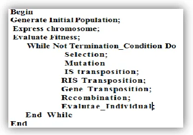
Fig 4: GEP Algorithm [25]
6.2
Genetic Operators.
Genetic operators are used to perform an interchange of information between chromosomes competing in the same population; they also introduce new genetic material that may not be present in the individuals. Genetic operators for GEP are described in following subsections.[24]
6.2.1 Mutation
Mutations are usually allowed to alter in any gene in the chromosome. Nevertheless, the structure of the chromosome must remain correct. When a mutation happens in the head domain, symbols can change into another function or terminal. However, as it takes place in the tail, terminal symbols can only change into terminals. In this manner, the structural organization for the chromosome is preserved, so the new chromosomes created by mutation are correct programs in their structure. A mutation occurs within a specific rate (pm) usually set to )0.05). Figure 5 shows what happens when a mutation occur in the head of a chromosome [25].
Fig 5: The Mutation Operation
6.2.2 Transposition and Insertion Sequence
elements
There are three types of this operation:
1- Insertion Sequence elements (IS): any sequence in the gene can form an (IS) element, so they are randomly selected throughout the chromosome. A copy is made of the transposition and is inserted at a random position in the head, except for the start position. The rate of an IS transposition (pis) is (0.1), a group of three different length IS elements are employed. IS randomly selects the chromosome, the starting position of the element, the target position, and the transposon’s length. [25] Through IS, the sequence from the copied IS element to the start will be changed; symbols equal to the length of the IS element will be eliminated from the end of the head. The
correctness of the resulting chromosome will still be maintained after this insertion.[21]
2- Root Insertion Sequence (RIS):Elements of RIS always start with a function; therefore they must be selected from the head domain. Usually a point in the head is chosen randomly and the gene is scanned forward to find a function, this function becomes the starting point of the RIS element. When no function is found, nothing is done. A root transposition rate (pris) is typically set to (0.1) and a group of three different size RIS elements are used. RIS randomly chooses the chromosome, the gene, RIS element starting point and length. [25]
3- Gene Transposition: - Here, the genes act as transposons and transpose themself to the starting point of the chromosome. Unlike the other forms of transposition, the transposon -the gene- is eliminated from its source location in order to maintain the length of the chromosome. The choice of chromosome to go through Gene transposition is random; a gene (apart from the first one) is randomly selected to be a transposon from that chromosome. Gene transposition rate is set to (0.0) because the chromosome composed of one gene.[25].
6.2.3 Recombination:
GEP usually has three types of recombination [25]:
1- One-point Recombination: A randomly chosen position is set to be the crossover point to produce two offspring chromosomes.This recombination is an important origin of genetic variation.
2- Two-point Recombination: it pairs the chromosomes and sets two points of recombination randomly. After that, the information between the recombination points are swapped between the two parents, materializing two new offspring chromosomes.
3- Gene recombination: here, genes are swapped between the parents, resulting in two new offspring chromosomes. This operator randomly selects the two parent chromosomes and the gene to be swapped [25]. In this recombination, the exchanged genes are very different most of the times, but this operator cannot create new genes, as the created chromosomes are just different arrangements of the existing genes [21].
The rate of each recombination operator is subject to the rates of other operators. Usually, a total crossover rate is set to (0.7) which denotes the summed rates of all kinds of recombination operators used
6.3
Fitness Function
The role of fitness functions is very critical when used in methods for problem solving, as the success of finding acceptable solutions to any given problem largely depends on the chosen fitness function and its suitability to the problem at hand. Therefore, the problem must be carefully studied to provide good insights for the selection process in the hope of finding better possible solutions.
For each chromosome in the population, the fitness is evaluated to figure out the chromosome’s performance and appropriateness. The fitness function can be measured in several ways; it can be represented as the error ratio between the actual input and the accomplished output. Or it might be measured via the involved (time or cost) required to achieve the desired goal. [24]
[image:4.595.56.281.456.599.2]the overall fitness for the individual will be the minimum fitness among the expressions encoded in that chromosome, as in Eq.(7).[27]
𝑓(𝐸𝑖) = 𝑛𝑘=1|𝑂𝑘,𝑖− 𝑊𝑘| ………(6)
where
Ok,i : is the result of expression Ei
Wk : is the actual output.
k: is the fitness case.
𝑓 𝐶 = min 𝑓 (𝐸𝑖) ……….………..(7)
6.4 Selection
In order to determine which of the chromosomes are to go through reproduction and genetic operators, a selection process is carried out to yield the offspring for the next new generation. This process is usually based on the fitness of the individuals, the more fit an individual is the more chance it has to be selected. In this research tournament selection was chosen to be selection method, and many Experiments were conducted to investigate the selection size used in the tournament selection, it proved that Tournament size (2) was better and give the best result[28].
7.
EXPERIMENTAL TESTING AND
RESULT
7.1
Datasets
An exploration has been carried out in this work to illustrate the ability of GEP in finding a function for estimating the software effort using the Datasets given in Table 1.
[image:5.595.53.276.471.661.2]The Datasets selected here provide variety and diversity, their availability and recurrent use made them become benchmark datasets in this field, and they are mostly used to carry out comparisons among techniques developed for software effort estimation.
Table 1 Dataset used in this work
No Dataset Name Total no of projects
1. Albrecht & Gaffney[29] [30]
5 incomplete (3,6,7,22,24) 24 points
2. Kemerer [31] 15 points
3. Desharnais[32] 4 incomplete (38,44,66,75)
77 points 4. NASA[14] 60 point
5. Miyazaki [33] 48 projects
6. Boehm[ 34] 63 projects
7. Kitchenham and Taylor[35]
33 projects
7.2
Parameters Setting
The preparation of GEP includes setting the parameter as follows:
Function Set: {-, +, *, /, POWER, EXP, LOG, SQRT}
Terminal Set: project’s variables depending on the Dataset NumGen :[25-1000]
PopSize : [10-500]
P(Mutation) :0.05
P(1-point) :0.3
P(2-point) : 0.4
7.3
Result Comparisons
7.3.1
Comparison with GP
Results of implementing GEP are compared with Genetic Programming for the same data [4]. The results in Table 2 show that the MMRE and PRED functions of GEP (shown in bold) are better than those of Genetic Programming. Table 3 shows the Effort Equations gained using GEP algorithm.
Table 2 Comparison between GP and GEP
No Dataset MMRE PRED(25)
GP GEP GP GEP
1
Miyazaki 0.50 0.43 47.9 502
Boehm 1.13 0.60 17.46 20.633
Kitchenham and Taylor0.84 0.51 27.27 36.36
Table 3 Effort Equation using GEP for the same dataset
No Dataset Effort Equation
1 Miyazaki E=)KLOC - log10(FILE((
2 Boehm E=(exp(VIRT) * KSLOC)
3 Kitchenham and Taylor E= (Schedular + Tes effort)
7.3.2
Comparison with Analogy:
Results of GEP algorithm are also compared to those obtained by Shepperd & Schofield [36] using analogy and stepwise regression.
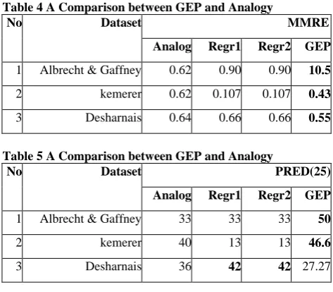
[image:5.595.314.551.510.717.2]Tables 4 and 5 show the results of comparing GEP’s results with those found by the Analogy method using (MMRE) and (PRED(25)) function. Results signify the efficiency of GEP, the best results of (MMRE) and (PRED) function of GEP are shown in bold. The Effort Equations of GEP for the same dataset are given in Table 6
Table 4 A Comparison between GEP and Analogy
No Dataset MMRE
Analog Regr1 Regr2 GEP
1 Albrecht & Gaffney 0.62 0.90 0.90 10.5
2 kemerer 0.62 0.107 0.107 0.43
3 Desharnais 0.64 0.66 0.66 0.55
Table 5 A Comparison between GEP and Analogy
No Dataset PRED(25)
Analog Regr1 Regr2 GEP
1 Albrecht & Gaffney 33 33 33 50
2 kemerer 40 13 13 46.6
Table 6 Effort Equations of GEP algorithm
No Dataset Effort Equation
1 Albrecht & Gaffney
E= (FP * sqrt((FP - sqrt(FILE))))
2 kemerer E =(FPcount / sqrt(sqrt(FPcount)))
3 Desharnais E=(YearEnd * (Envergure + TeamExp))
7.3.3
Comparison with COCOMO:
[image:6.595.50.283.74.164.2]A comparison was conducted with the known empirical models (Intermediate COCOMO) [19], results show the success of the GEP as shown in Table 7. Table 8 shows the Effort Equation of GEP for NASA data.
Table 7 A Comparison between GEP and COCOMO
Dataset
MMRE
COCOMO Model GEP
NASA 0.36 0.30
Table 8 Effort Equation for the NASA Dataset
COCOMO GEP ( MMRE=0.30)
E =𝑎 (𝐾𝑆𝐿𝑂𝐶)𝑏 𝐸𝑀 𝑖 15
𝑖=1 E=((LEXP + exp((PCAP/
LEXP))) * KSLOC)
7.3.4
Comparisons with Neural Networks:
In the end, and for further investigation, GEP is compared with four types of Neural Networks, they are as follows[14]:
The Cascade Neural Network (CNN).
The Radial Basis Functions Network (RBFN(.
The Feed Forward Neural Network (FFNN).
The Elman Neural Network (ENN).
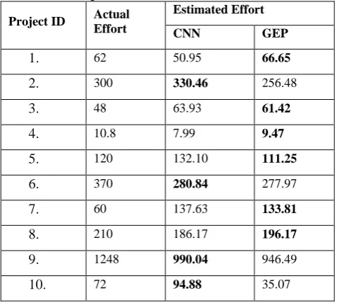
[image:6.595.53.270.233.375.2]Tables 9 through 12 show the results of GEP and the four Neural Networks taken for comparisons, these results indicate the superiority of GEP over others in 6 cases out of 10 most of the times.
Table 9 A Comparison between GEP and CNN
Project ID Actual Effort
Estimated Effort
CNN GEP
1.
62 50.95 66.652.
300 330.46 256.483.
48 63.93 61.424.
10.8 7.99 9.475.
120 132.10 111.256.
370 280.84 277.977.
60 137.63 133.818.
210 186.17 196.179.
1248 990.04 946.4910.
72 94.88 35.07Table 10 A Comparison between GEP and RBFN Project ID Actual
Effort
Estimated Effort
RBFN GEP
1.
62 70.3 50.882.
300 331.8 247.963.
48 22 55.784.
10.8 10.9 19.025.
120 127.8 113.356.
370 195.1 197.367.
60 211.7 111.368.
210 156.5 133.729.
1248 1579.4 587.7110.
72 20.9 30.372Table 11 A Comparison between GEP and FFNN Project ID Actual
Effort
Estimated Effort
FFNN GEP
1.
62 55.18 64.612.
300 331.00 278.693.
48 58.57 62.764.
10.8 46.26 14.645.
120 115.17 123.446.
370 286.24 221.667.
60 136.08 131.818.
210 184.79 175.659.
1248 981.30 1091.5710.
72 72.94 53.94Table 12 Comparison between GEP and ENN Project ID Actual Effort Estimated Effort
ENN GEP
1.
62 58.8 31.52.
300 355.6 295.83.
48 38.9 40.94.
10.8 38.3 15.55.
120 109.8 131.06.
370 234 260.87.
60 161.5 85.98.
210 158.5 183.369.
1248 1018.3 575.31 [image:6.595.48.287.524.738.2]8.
CONCLUSION
Effort estimation was investigated in this work using the Gene Expression Programming (GEP) method. This artificial intelligent technique was adopted to find estimation functions suitable enough to give best estimates based on the training sets provided be previous projects.
GEP was employed to bypass the complications of Genetic Programming such as tree size and depth, and to guarantee that solutions are still correctly functioning following the genetic operations.
In order to evaluate this employment, some comparisons were performed between GEP and other methods including (GP, Analogy, COCOMO, and Neural Networks. The results showed that GEP was far better than the previously mentioned methods using the same datasets.
9.
REFERENCES
[1] Roger S. Pressman,( 2010), "Software Engineering A Practitioner’s Approach, Seventh Edition", 7th
, McGraw-Hill Company.
[2] Mohanty, S.K., Bisoi, A.K., (2012), ”Software Effort Estimation Approaches – A Review”, International Journal of Internet Computing ISSN No: 2231 – 6965, VOL- 1, ISS- 3.
[3] Singh, J., Sahoo ,B., (2011), "Software Effort Estimation with Different Artificial Neural Network", IJCA, 2nd National Conference- Computing, Communication and Sensor Network” CCSN.
[4] Dolado J.J., (2001),”On the problem of the software cost function”, Information and Software Technology, pp: Elsevier Science B.V. All rights reserved
[5] Zhiwei, Xu, and Taghi, M. Khoshgoftaar (2004). Identification of fuzzy models of software cost estimation. In Fuzzy Sets and Systems, V.145, Issue 1, 1 July 2004, Pages 141-163.
[6] Carroll, E. R. (2005). Estimating software based on use case points. In Companion to the 20th annual ACM SIGPLAN conference on Object-oriented programming, systems, languages, and applications. pp: 257-265. ACM.
[7] Huang, S., Chiu, N. (2006),”Optimization of Analogy Weights by Genetic Algorithm for Software Effort Estimation”, Journal of Systems and Software 48 (11), pp:1034-1045.
[8] Mendes, E., Mosley, N., (2008). “Bayesian Network Models for Web Effort Prediction: A Comparative Study”. IEEE Trans. SWE, 34(6), pp: 723-737.
[9] Uzoka, F. M. E. (2009). Fuzzy-Expert system for cost Benefit Analysis of Enterprise information systems, A Frame work. International Journal on Computer Science and Engineering, 1(3), pp: 254-262.
[10]Ramesh, S. N. S. V. S. C. (2010). Software effort estimation using radial basis and generalized regression neural networks. Journal of Computing, 2(5), ISSN 2151-9617 arXiv preprint arXiv:1005.4021.
[11]Azzeh, M. (2011). Model Tree Based Adaption Strategy for Software Effort Estimation by Analogy. In Computer and Information Technology (CIT), 2011 IEEE 11th International Conference on (pp. 328 –335). doi:10.1109/CIT.2011.48
[12]Ziauddin, Sh., Kamal, T., Shahrukh, Z., (2012) “An Effort Estimation Model for Agile Software Development,” Advances in Computer Science and Its Applications (ACSA), Vol.2, No.1, pp. 314-324. [13]Toka, D., Turetken, O. (2013). Accuracy of
Contemporary Parametric Software Estimation Models:
A Comparative Analysis. 39th Euromicro Conference on Software Engineering and Advanced Applications SEAA
2013 IEEE, 313- 316.
http://dx.doi.org/10.1109/SEAA.2013.49
[14]Quba, I., Z. (2012). “Software Projects Estimation using Neural Networks”. M.Sc Thesis. College of Computers Sciences & Mathematics , University of Mosul. (in Arabic).
[15]Arnuphaptrairong, T., (2013),” Early Stage Software Effort Estimation Using Function Point Analysis: Empirical Evidence”, Proc. of the Inter. Multi-Conf. of Engineers and Computer Scientists Vol. II, (IMECS), March 13-15, Hong Kong. pp: 730-735.
[16]Puri, R., Kaur, I., (2015) “Novel Meta-Heuristic Algorithmic Approach for Software Cost Estimation”. In I. J. of Innovations in Engineering and Technology (IJIET), Vol. (5), Issue-2.
[17]Sharma, Sh., Kaushik, A., and Tomar, A., (2016) “Software Cost Estimation using Hybrid Algorithm”. In I. J. of Engineering Trends and Technology (IJETT). Vol. (37), No.2.
[18]Chetan Nagar, Anurag Dixit, 2011, "Software Efforts and Cost Estimation with a Systematic Approach", ISSN, Journal of Emerging Trends in Computing and Information Sciences.
[19]Kaushik ,A., Chauhan, A., Mittal, D.,Gupta, S.,)2012(,” COCOMO Estimates Using Neural Networks” , MECS DOI: 10.5815/ijisa.2012.09.03,© MECS I.J. Intelligent Systems and Applications.
[20]Nancy Merlo, Schett, (2002)," COCOMO (Constructive Cost Model)", Requirements Engineering Research Group, Department of Computer Science, University of Zurich, Switzerland.
[21]Fan,W., Fox, E.,A. , Pathak, P., Wu H.,2004 ,” The Effects of Fitness Functions on Genetic Programming-Based Ranking Discovery For Web Search “,Journal of the American Society for Information Science and Technology,27-14 self.
[22]Sheta A.F., Al-Afeef A., (2010). “A GP Effort Estimation Model Utilizing Line of Code and Methodology for NASA Software Projects”, In proceeding of: 10th International Conference on Intelligent Systems Design and Applications, ISDA, pp: 290-295.
[23]Oltean, M., Dumitrescu, D., (2002) “Multi Expression Programming”.Technical-Report,UBB-01-2002. [24]AL-Saati, N., A. , Alreffaee, T., R.,(2017), " Using Muli
Expression Programming in Software Effort Estimation", International Journal of Recent Research and Review, Vol. X, Issue 2, June 2017, ISSN 2277 – 8322.
[25]Ferreira, C., (2001),” Gene Expression Programming: A new Adaptive Algorithm for Solving Problems”, Complex Systems, Vol. 13, issue 2: 87-129, 2001. [26]Jarullah, T.R. (2017). “Software Effort Estimation using
evolutionary computation”. M.Sc Thesis. College of Computers Sciences & Mathematics, University of Mosul. (in Arabic).
[27]Oltean, M.,(2006),“Multi Expression Programming”. Tech.l Report, Babes-Bolyai Univ, Romania.28p. [28]Miller, B.L., Goldberg, D.E., (1995). "Genetic
Algorithms, Tournament Selection, and the Effects of Noise". Complex Systems. 9: 193–212.
[29]http://code.google.com/p/promisedata/wiki/Albrecht [30]Albrecht, A.J., Gaffney, J.R., (1983),” Software
[31]Kemerer, C.F., (1987), “An Empirical Validation of Software Cost Estimation Models”, Communications of the Association for Computing Machinery 30 (5). pp:416–429.
[32]Desharnais, J.M., (1988), “Analyse statistique de la productivite´ des projects de de´velopment en informatique a` partir de la technique des points de function”, Master’s Thesis, Univ. du Que´bec a` Montreal, De´cembre,.
[33]Miyazaki, Y., Terakado, M., Ozaki, K., Nozaki, H., (1994), “Robust regression for developing software estimation models”, J. of Sys..& SW 27 (1),pp:3–16.
[34]Boehm, B.W., Software Engineering Economics, Prentice-Hall, Englewood Cliffs, NJ, 1981.
[35]B.A. Kitchenham, N.R. Taylor, Software project development cost estimation, Journal of Systems and Software 5 (1985) 267–278.
![Fig 3: Gene Expression Programming Representation [26]](https://thumb-us.123doks.com/thumbv2/123dok_us/9292733.425866/3.595.55.260.441.618/fig-gene-expression-programming-representation.webp)