A Bayesian Filter for Sound Environment System with Quantized Observation*

(1)

ISSN Online: 2160-5920 ISSN Print: 2160-5912

DOI: 10.4236/iim.2018.103007 May 25, 2018 87 Intelligent Information Management

A Bayesian Filter for Sound Environment

System with Quantized Observation

*

Hisako Orimoto, Akira Ikuta

Department of Management Information Systems, Prefectural University of Hiroshima, Hiroshima, Japan

Abstract

In the real sound environment, the observation data are usually contaminated by additional background noise of arbitrary distribution type. In order to es-timate several evaluation quantities for specific signal based on the observed noisy data, it is fundamental to estimate the fluctuating wave form of the spe-cific signal. On the other hand, the observation data are very often measured in a digital level form at discrete times. This is because some signal processing methods by utilizing a digital computer are indispensable for extracting ex-actly various kinds of statistical evaluation for the specific signal based on the quantized level data. In this study, a Bayesian filter matched to the compli-cated sound environment system is derived. First, in the real situation where the sound environment system is affected by background noise of arbitrary probability distribution, a stochastic system model with quantized observation is established. Next, two types of the recursive algorithm of Bayesian filter to estimate the unknown specific signal are theoretically proposed in the quan-tized level form. Finally, the effectiveness of the proposed theory is experi-mentally confirmed by applying it to the estimation problem of real sound environment.

Keywords

Bayesian Filter, Sound Environment, Quantized Observation

1. Introduction

In the real sound environment, the observation data are usually contaminated by additional external noise (i.e., background noise) of arbitrary distribution type. In order to estimate several evaluation quantities for specific signal, like Lx

*New type method is proposed based on the Baysian filter by use of the quantized observation in sound environment system.

How to cite this paper: Orimoto, H. and Ikuta, A. (2018) A Bayesian Filter for Sound Environment System with Quan-tized Observation. Intelligent Information Management, 10, 87-98.

https://doi.org/10.4236/iim.2018.103007

Received: April 23, 2018 Accepted: May 22, 2018 Published: May 25, 2018

(2)

DOI: 10.4236/iim.2018.103007 88 Intelligent Information Management

((100−x_{) percentile level),}L_eq (averaged energy on decibel scale) and peak value, based on the observed noisy data, it is fundamental to estimate the mo-mentarily fluctuating wave form of the specific signal.

Up to now, many methodological studies have been reported on the state es-timation for stochastic systems [1] [2] [3]. However, many standard estimation methods proposed previously in a study of stochastic systems are restricted only to the Gaussian distribution [4] [5]. Several state estimation methods for nonli-near system have been also proposed by assuming the Gaussian distribution of system and observation noises [6] [7] [8] [9] [10]. The real sound environment often shows an intricate fluctuation pattern rather than the standard Gaussian distribution. In our previous studies [11] [12] [13] [14] [15], several state esti-mation methods for a sound environment system with non-Gaussian fluctua-tions have been proposed on the basis of expansion expressions for the probabil-ity distribution. Furthermore, state estimation methods for stochastic systems with complex characteristics and/or unknown structure have been proposed by using Bayes theorem on probability distribution [16] [17] [18]. Especially, though the unscented Kalman filter (UKF) and particle filter are useful for non-linear systems, UKF considers only the mean and variance of variables, and the particle filter needs very complicated algorithm based on Monte Carlo simu-lation [10] [18].

On the other hand, in the actual case contaminated by the background noise, some signal processing methods utilizing a digital computer are indispensable for estimating precisely the latent specific signal based on the noisy observations. Therefore, the observed data in an analogue form have to be transformed into a digital one at discrete time. However, many standard estimation methods pro-posed previously in stochastic systems are restricted only to a continuous level form of the observation.

(3)

2. Formulation of Sound Environment System with

Quantized Observation

Let us consider an arbitrary stochastic environment system with the power state variables of arbitrary distribution type, and express the system equation as:

1

k k k

x+ =Fx Gu+ (1)

where xk denotes the specific signal at a discrete time k, uk is the random input with known statistics. Here, xk and uk are statistically independent of each other. Two parameters F and G are estimated by using an auto-correlation technique [1]. Furthermore, the observation model is established by considering the additive property of power variables and the quantized observation in deci-bel scale, as follows:

(

)

{

12

}

10

10log 10

k k k

y ₌ x ₊v − ₍₂₎

( )

(

)

k k k k

z =Q y ≡g x +v (3)

where yk is the noisy observation contaminated by the additive background noise vk. Though yk is decibel variable with continuous level, the observation data are measured in a quantized level form suitable for the signal processing by use of a digital computer through A/D converter. The function Q y

( )

k denotes

a nonlinear function expressing the quantization mechanism and zk is the quantized observation. Therefore, g v

( )

denotes a nonlinear function com-bining the nonlinearity of decibel observation with the quantized observation mechanism. In this study, a Bayesian filter to estimate the specific signal xk is proposed on the basis of the quantized observation contaminated by the back-ground noise vk.

3. Establishment of Bayesian Filter with Quantized

Observation

3.1. General Expression of Bayesian Filter in Expansion Series

Form

In order to express explicitly the effect of successive observation zk on the es-timated probability density function P x Z

(

k| k

)

by use of various types of

li-near and/or nonlili-near correlation between xk and zk, the well-known Bayes’ theorem is introduced.

(

k| k

)

(

k, |k k1

) (

k| k1

)

P x Z =P x z Z− P z Z − (4)

where

(

Zk≡

{

z z1, , ,2 zk

}

)

is a set of observation data up to time k. By

ex-panding the conditional probability density function P x Z

(

k| k

)

in a statistical

orthogonal expansion series on the basis of the well-known standard probability distributions describing the dominant part of the actual fluctuation, the follow-ing expression is derived [11] [12].

(

)

(

)

( )

_{( )}

( )

_{( )}

( )

_{( )}

1 2

0 1

0 0 2 0 0 |

| k k m n mn m k n k

k k

n n k n

P x Z A x z

P x Z

A z

φ φ

φ

∞ ∞

−

= =

∞

=

∑ ∑

(4)

with

( )

_{( )}

( )

_{( )}

1

1 2

m n k

n k k

m x

A ≡ φ φ z Z₋ ₍₆₎

The above two functions ( )1

( )

m xk

φ and ( )2

( )

n zk

φ are orthonormal polyno-mials of degrees m and n with weighting functions P x Z0

(

k| k−1

)

and

(

)

0 k| k1

P z Z − . Based on Equation (5), the estimate of the polynomial function

( )

M k

f x of xk with Mth order can be derived as follows.

( )

( )2

_{( )}

( )2

_{( )}

0

0 0 0

ˆ_M _k _M _k _k

M

Mm mn n k n n k

m n n

f x f x Z

C A φ z A φ z

∞ ∞

= = =

≡

=

∑ ∑

∑

(7)

where CMm is an appropriate constant satisfying the following equality:

( )

( )1

_{( )}

0

M

M k Mm m k

m

f x C φ x

=

∑

₍₈₎

3.2. Estimation Algorithm by Introducing Difference Operation

In order to make the general theory for estimation algorithm more concrete, Gaussian distribution is considered as an example of standard probability func-tions for the specific signal:

(

)

(

*

)

0 k| k1 k; ,k xk P x Z− =N x x Γ

(

2

)

(

)

2

2 2

1

; , exp

2 2π

x

N x

µ σ

µ

σ

 ₋    ≡ _− _    , * 1 k k x k

x ≡ Z − ,

(

)

2 *

1

k

x xk xk Zk−

Γ ≡ − (9) Furthermore, as the fundamental probability function on the level-quantized observation, the generalized binomial distribution [19] with level difference in-terval hz can be chosen:

(

)

(

)

0 1

!

| 1

! !

k M _k _k

z _z

k M

z z _{N z}

z h _h

k k k k

k M k k

z z

N z

h

P z Z p p

z z N z

h h − ₋ −  −      = −  −   −          * k M k k M z z p N z − ≡ − ,

(

)

(

)

* * * k k k M z k M z k

k M z z

z z h z z

N

z z h

− − Ω ≡

− − Ω

*

1

k k k

z ≡ z Z− ,

(

)

2 *

1

k

z zk zk Zk−

Ω ≡ − ₍₁₀₎

where zM is the minimum level of observations. The orthonormal polynomials with two weighting probability distributions in Equations (9) and (10) can be determined as

( )1

_{( )}

1 *

! _k

k k

m k m

x

x x

x H

m

φ =  −   Γ 

(5)

( )

_{( )}

( )

(

)

( )

₍

₎

( )

1 2 ₂

2 0 1 1 ! 1 1 n n

k M k

n k n

z k z

n j

n _{n j} _{n j} _j

k

k k k M

j k

N z p

z n

h p h

n p _N _z _z _z

j p φ − − − − = _ ₋ _  _ ₋ _   =                  ⋅   −  ₋  − −    

∑

(12)

where Hm

( )

⋅ denotes the Hermite polynomial with mth order, and z( )j is the

jth order factorial function defined by [19]

( )n

₍

₎₍

₂

₎

₍

₁

₎

_, ( )0 ₁

z z z

z =z z h z− − h ⋅⋅⋅ −z n− h z = (13) Since the function g

( )

⋅ in Equation (3) is not differentiable in general, the following expansion expression of discrete type is introduced with two arbitrary constants dv and hv.

(

)

( )

_{( )}

0 1 ! n n n v n v d

g x v x g v

n h ∞ =   + = _ _ ∆  

∑

(14)

where ∆ is the forward difference operator defined as:

( )

1

{

(

v

)

( )

}

v

g v g v h g v

d

∆ ≡ + − ₍₁₅₎

After substituting Equations (2) and (3) into the definition of two parameters of zk and Ωzk in Equation (10), by applying Equation (14), the following ex-pressions can be derived (in the case of dv=hv).

(

)

( )

(

)

( )

* 1 2 1 1 2

k k k k

k k k k k v k k

z g x v Z

g v x g v x x h g v Z

−

= +

= + ∆ + − ∆ + ⋅⋅⋅ (16)

(

)

{

}

( )

(

)

( )

2 * 1 2 2 * 1 1 2 k

z k k k k

k k k k k v k k k

g x v z Z

g v x g v x x h g v Z z

−

Ω = + −

 

=  + ∆ + − ∆ + ⋅⋅⋅ −

 

(17)

Furthermore, the expansion coefficients defined by Equation (6) can be ex-pressed as follows:

( )

(

)

(

)

( )

₍

₎

( )

1 2 ₂

0

*

1

1 1

! ! 1

1

k

n n j

n _n

n j

k M k k

mn n

j

z k z k

n j j

k k

m k k k k k M k

x

n

N z p p

A m n

j

h p h p

x x

H N g x v g x v z Z

− ₋ − = − − _ ₋ _  _ ₋ _ _{ } _ _   =       −  ₋               ₋    ⋅ − + + −

 Γ   

∑

(18)

The above Equations (16)-(18) can be obtained from the statistics of the background noise vk and the predictions of xk at a discrete time k−1; i.e., the expectation values of arbitrary functions of xk conditioned by Zk−1.

(6)

( )

(

)

( )

₍

₎

( )

1 2 ₂

0 0 0 1 1 ˆ _! 1 1 n n M

k M k

M k Mm mn n

m n z k z

n j

n _{n j} _{n j} _j

k

k k k M

j k

N z p

f x C A n

h p h

n p _N _z _z _z _I

j p − ∞ = = − − − = _ ₋ _  _ ₋ _   = __ _ _ _ _             ⋅ _{ } − _ _ − − −    

∑ ∑

∑

(19) with ( )

( )

(

)

( )

₍

₎

( )

1 2 ₂

0 0 0 1 1 ! 1 1 n n

k M k

n n

n z k z

n j

n _{n j} _{n j} _j

k

k k k M

j k

N z p

I A n

h p h

n p _N _z _z _z

j p − ∞ = − − − = _ ₋ _  _ ₋ _   =                  ⋅   −  ₋  − −    

∑

(20)

Especially, the estimates for mean and variance can be obtained as follows:

( )

(

)

( )

₍

₎

( )

(

)

1 2 ₂

1 1 0 0 0 * 10 11 ˆ 1 1 ! 1 1 , _k

k k k

n n

k M k

m mn n

m n z k z

n j

n _{n j} _{n j} _j

k

k k k M

j k

k x

x x Z

N z p

C A n

h p h

n p _N _z _z _z _I

j p

C x C

− ∞ = = − − − = ≡ _ ₋ _  _ ₋ _   = __ _ _ _ _             ⋅ _{ } − _ _ − − −    

= = Γ

∑ ∑

∑

(21)

(

)

( )

(

)

( )

₍

₎

( )

(

)

(

)

(

)

2

1 2 ₂

2 2 0 0 0 2 * *

20 21 22

ˆ

1 1

!

1 1

ˆ , 2 ˆ , 2

k k k

k k k k

n n

k M k

m mn n

m n z k z

n j

n _{n j} _{n j} _j

k

k k k M

j k

x k k x k k x

P x x Z

N z p

C A n

h p h

n p _N _z _z _z _I

j p

C x x C x x C

− ∞ = = − − − = ≡ − _ ₋ _  _ ₋ _   = __ _ _ _ _             ⋅   −  ₋  − −    

= Γ + − = Γ − = Γ

∑ ∑

∑

(22)

3.3. Estimation Algorithm by Introducing Particles

Though the particle filter is useful for the state estimation problem of non-linear systems, this filter needs very complicated algorithm and a large number of computational times based on Monte Carlo simulation and the resampling pro-cedure [16]. In this section, a hybrid algorithm combining the analytical formula for state estimation with Monte Carlo simulation by use of particles is proposed.

The well-known Gaussian distribution is adopted as P x Z0

(

k| k−1

)

and

(

)

0 k| k1

P z Z − , because this probability density function is the most standard one.

(

)

(

*

)

0 k| k1 k; ,k xk

(7)

( )1

_{( )}

1 *

! _k

k k

m k m

x

x x

x H

m

φ =  −   Γ   ,

( )2

_{( )}

1 *

! _k

k k

n k n

z

z z

z H

n

φ =  −   Ω 

  (24)

Accordingly, the estimation algorithm of the specific signal in Equation (7) can be given by

( )

* 0 0 1 ˆ ! _k M k k

M k Mm mn n

m n _z

z z

f x C A H J

n ∞ = =  ₋    =

 Ω   

∑ ∑

(25)

with * 0 0 1 ! _k k k n n n _z z z

J A H

n ∞ =  ₋    =

 Ω   

∑

(26)

Furthermore, the estimates for mean and variance can be obtained as follows:

* 1 1 0 0 1 ˆ ! _k k k

k m mn n

m n z

z z

x C A H J

n ∞ = =  ₋    =

 Ω   

∑ ∑

(27)

* 2 2 0 0 1 ! _k k k

k m mn n

m n _z

z z

P C A H J

n ∞ = =  ₋    =

 Ω   

∑ ∑

(28)

Thus, two parameters * k

z , Ωz_k and the expansion coefficients Amn are ex-pressed as follows:

(

)

(

) (

) ( )

*

1

| d d

k k k k

k k k k k k k

z g x v Z

g x v P x Z P v x v

−

= +

=

_∫∫

+ (29)

(

)

(

)

(

)

(

)

(

) ( )

2 * 1 2 * 1

| d d

k

z k k k k

k k k k k k k k

g x v z Z

g x v z P x Z P v x v

−

Ω = + −

=

_∫∫

+ − (30)

(

)

(

)

₍

_{) ( )}

* * 1 * * 1 1 1 ! !

1 1 _| _{d d}

! !

k k

k k k

k k

mn m n k

x z

k k k

k k

m n k k k k k

x z

g x v z

x x

A H H Z

m n

g x v z

x x

H H P x Z P v x v

m n − −  ₋   ₊ ₋      =

 Γ   Ω 

   

 ₋   ₊ ₋ 

   

=

 Γ   Ω 

   

∫∫

(31) The integrals in Equations (29)-(31) are evaluated by use of particles with mean *

k

x , variance Γ_x_k, higher order statistics Am0 and statistics of the

back-ground noise.

3.4. Prediction Algorithm

By considering Equation (1), the prediction step essential to perform the recur-rence estimation can be given by

*

1 1 ˆ

k k k k k

(8)

(

)

(

)

1

2 2

* 2 2

1 1

k

x+ xk+ xk+ Zk F P Gk uk uk

Γ ≡ − = + − (33)

By replacing k with k+1_{, the recurrence estimation can be achieved.}

4. Application to Sound Environment

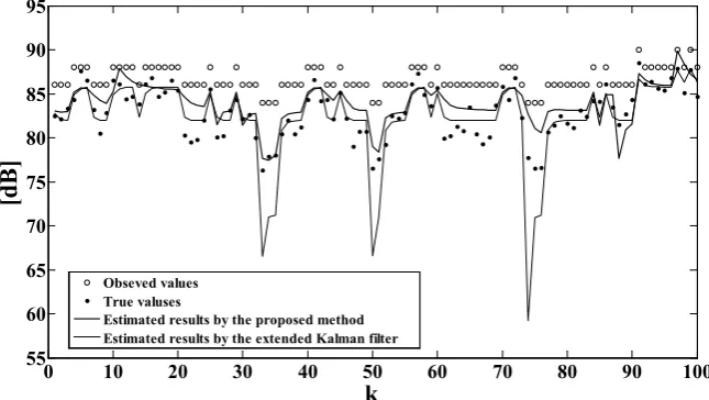
In order to examine the practical usefulness of the proposed Bayesian filter based on the quantized observation, the proposed method is applied to the actual sound environmental data. The road traffic noise is adopted as an example of a specific signal with a complex fluctuation form. Applying the proposed estima-tion method to actually observed data contaminated by background noise and quantized with 2 dB width roughly, the fluctuation wave form of the specific signal is estimated. The statistics of the specific signal and the background noise used in the experiment are shown in Table 1 and Table 2 respectively.

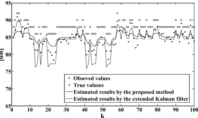
[image:8.595.212.535.328.510.2]

Figure 1 and Figure 2 show the estimation results of the fluctuation wave form of the specific signal for Data 1 and Data 2 by applying the algorithm pro-posed in Secttion 3.2. In this estimation, the finite number of expansion

[image:8.595.209.542.577.628.2]

Figure 1. Estimation results for Data 1 of the specific signal by applying the proposed method in Section 3.2 based on the quantized observation data with 2 dB width.

Table 1. Mean and standard deviation of the specific signal (in W/m2_).

Data Data 1 Data 2 Data 3 Data 4 Data 5

Mean Value 2.23 × 10−4 _{3.44 × 10}−4 _{3.25 × 10}−4 _{3.82 × 10}−4 _{3.71 × 10}−4

[image:8.595.210.541.663.717.2]

Standard Deviation 1.47 × 10−4 _{2.13 × 10}−4 _{2.65 × 10}−4 _{3.19 × 10}−4 _{3.56 × 10}−4

Table 2. Mean and standard deviation of the background noise (in W/m2_).

Mean Value 2.50 × 10−4 _{2.49 × 10}−4 _{2.44 × 10}−4 _{2.47 × 10}−4 _{2.48 × 10}−4

Standard Deviation 1.08 × 10−5 _{9.61 × 10}−6 _{9.49 × 10}−6 _{1.05 × 10}−5 _{9.26 × 10}−6

0 10 20 30 40 50 60 70 80 90 100

55 60 65 70 75 80 85 90 95

k

[d

B

]

Obseved values True valuses

(9)

coefficients A m nmn

(

, ≤2

)

is used for the simplification of the estimation

algo-rithm. In these figures, the horizontal axis shows the discrete time k, of the esti-mation process, and the vertical axis expresses the sound level taking a logarith-mic transformation of power-scaled variables, because the actual sound envi-ronment usually is evaluated on dB scale. For comparison, the estimation results calculated by using the usual method are also shown in these figures. Since Kal-man’s filtering theory is widely used in the field of stochastic system [11] [12], the extended Kalman filter is also applied to the observation data as a trail by in-troducing the following observation model.

(

)

12

10

10log 10

k k k k

z ₌ x v₊ − ₊ε ₍₃₄₎

where εk denotes the quantized noise and a uniform distribution within

[

−q 2, 2q

]

₍_q_{: the quantized width) is assumed as the probability distribution}

of εk. The results estimated by the proposed method show good agreement with the true values. On the other hand, there are great discrepancies between the estimates based on the standard type dynamical estimation method (i.e., ex-tended Kalman filter), particularly in the estimation of the lower level values of the fluctuation.

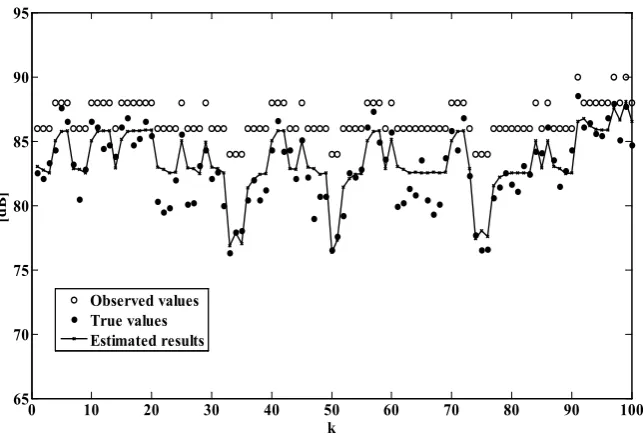
Furthermore, the estimation algorithm proposed in Section 3.3 is applied to the observation data. The estimated results of two cases by applying the pro-posed algorithm to the quantized data with 2 dB width are shown in Figure 3

and Figure 4 respectively.

The squared sums of the estimation error are shown in Table 3. It can be found numerically that the proposed method is more useful than the extended Kalman filter.

5. Conclusions

In this study, state estimation method for sound environment system with

0 10 20 30 40 50 60 70 80 90 100

65 70 75 80 85 90 95

k

[d

B

]

Obseved values True valuses

[image:9.595.215.536.71.262.2]

(10)

[image:10.595.214.536.69.286.2]

[image:10.595.211.534.334.548.2]

Table 3. Comparison between the proposed method and the extended Kalman filter for root-mean squared error of the estimation based on the quantized observation data with 2 dB width (in dB).

Proposed Method in Section 3.2 2.06 1.73 2.14 2.08 2.67

Proposed Method in Section 3.3 1.39 1.09 1.81 1.87 2.24

Extended Kalman Filter 2.96 1.75 1.88 2.23 3.36

0 10 20 30 40 50 60 70 80 90 100

65 70 75 80 85 90 95

k

[d

B]

Observed values True values Estimated results

0 10 20 30 40 50 60 70 80 90 100

65 70 75 80 85 90 95

k

[d

B]

[image:10.595.209.541.639.719.2]

(11)

quantized level observation has been theoretically proposed on the basis of Bayes’ theorem. More specifically, two types of the recursive algorithm of Baye-sian filter to estimate the specific unknown signal have been derived based on the quantized level observation matched for the signal processing by use of a digital computer. Furthermore, the validity and effectiveness of the proposed theory have been experimentally confirmed by applying it to the real environ-mental noise data in sound environment.

The proposed approach is still at the early of study, and there are left a num-ber of practical problems to be continued in the future. For example, the pro-posed method has to be applied to many other actual data of sound environ-ment. Furthermore, the proposed theory has to be extended to more compli-cated situations involving multi-signal sources, and an optimal number of ex-pansion terms in the proposed estimation algorithm of exex-pansion type has to be found.

Acknowledgements

The author is grateful for valuable suggestions at Inter-Noise 2016 [20]. This work was supported in part by fund from the Grant-in-Aid for Scientific Re-search No.15K06116 from the Ministry of Education, Culture, Sports, Science and Technology-Japan.

References

[1] Eykhoff, P. (1974) System Identification: Parameter and State Estimation. Wiley, New York.

[2] Young, P. (1984) Recursive Estimation and Time-Series Analysis. Springer-Verlag, Berlin. https://doi.org/10.1007/978-3-642-82336-7

[3] Gremal, M.S. and Andrews, A.P. (1993) Kalman Filtering-Theory and Practice. Prentice-Hall, New Jersey.

[4] Kalman, R.E. (1960) A New Approach to Linear Filtering and Prediction Problems.

ASME, Series D, Journal of Basic Engineering, 82, 35-45.

https://doi.org/10.1115/1.3662552

[5] Kalman, R.E. and Buch, R.S. (1961) New Results in Linear Filtering and Prediction Theory. Transactions on ASME, Series D, Journal of Basic Engineering, 83, 95-108.

https://doi.org/10.1115/1.3658902

[6] Kushner, H.J. (1967) Approximations to Optimal Nonlinear Filter. IEEE Transac-tions on Automatic Control, 12, 546-556.

https://doi.org/10.1109/TAC.1967.1098671

[7] Bell, B.M. and Cathey, F.W. (1993) The Iterated Kalman Filter Update as a Gauss-Newton Methods. IEEE Transactions on Automatic Control, 38, 294-297.

https://doi.org/10.1109/9.250476

[8] Nishiyama, K. (1997) A Nonlinear Filter for Estimating a Sinusoidal Signal and Its Parameter: On the Case of a Single Sinusoid. IEEE Transactions on Signal Processing, 45, 970-981. https://doi.org/10.1109/78.564185

(12)

DOI: 10.4236/iim.2018.103007 98 Intelligent Information Management 509-520.

[10] Julier, S.J. (2002) The Scaled Unscented Transformation. Proceedings of the Amer-ican Control Conference, 6, 4555-4559. https://doi.org/10.1109/ACC.2002.1025369

[11] Ohta, M. and Yamada, H. (1984) New Methodological Trials of Dynamical State Es-timation for the Noise and Vibration Environmental System—Establishment of General Theory and Its Application to Urban Noise Problems. Acustica, 55, 199-212. [12] Ikuta, A. and Ohta, M. (1992) A State Estimation Method of Impulsive Signal Using

Digital Filter under the Existence of External Noise and Its Application to Room Acoustics. IEICE Transactions on Fundamentals of Electronics, Communications and Computer Sciences, E75, 988-995.

[13] Ikuta, A., Ohta, M. and Masuike, H. (2006) A Countermeasure for an External Noise in the Measurement of Sound Environment and Its Application to the Evalu-ation for Traffic Noise at Main Line. IEEJ Transactions on EIS, 126, 63-71.

https://doi.org/10.1541/ieejeiss.126.63

[14] Orimoto, H., Ikuta, A. and Xiao, Y. (2016) Method for Evaluating the Statistical Re-lationship between Sound Pressure Level and Noise Annoyance Based on a Nonli-near Time Series Regression Model and an Experiment. International Journal of Acoustics and Vibration, 21, 145-151. https://doi.org/10.20855/ijav.2016.21.2403

[15] Ikuta, A., Orimoto, H. and Gallagher, G. (2017) State Estimation for Fuzzy Sound Environment System with Finite Amplitude Fluctuation. Journal of Software Engi-neering and Applications, 10, 625-638. https://doi.org/10.4236/jsea.2017.107034

[16] Habbibi, B., Sayed, A.H. and Kailath, T. (1996) Linear Estimation in Krein Spac-es—Parts I Theory and II Applications. IEEE Transactions on Automatic Control, 41, 18-33, 34-49.https://doi.org/10.1109/9.481605

[17] Ikuta, A., Masuike, H. and Ohta, M. (2007) State Estimation for Sound Environ-ment System with Unknown Structure by Introducing Fuzzy Theory. The Institute of Electrical Engineers of Japan, 127, 770-777.

https://doi.org/10.1541/ieejeiss.127.770

[18] Kitagawa, G. (1996) Monte Carlo Filter and Smoother for Non-Gaussian Nonlinear State Space Models. Journal of Computational and Graphical Statistics, 5, 1-25. [19] Ikuta, A., Ohta, M. and Ogawa, H. (1997) Various Regression Characteristics with

Higher Order among Light, Sound and Electromagnetic Waves Leaked from VDT—Measurement and Signal Processing in the Actual Working Environment.

International Measurement Confederation, 21, 25-33. https://doi.org/10.1016/S0263-2241(97)00041-9