Class specific synthesized dictionary model for Zero Shot Learning

Class-Specific Synthesized Dictionary Model for Zero-Shot Learning

Zhong Jia,∗, Junyue Wanga_{, Yunlong Yu}a,∗_{, Yanwei Pang}a_{, Jungong Han}b

a_{School of Electrical and Information Engineering, Tianjin University, China} b_{School of Computing and Communications, Lancaster University, UK}

Abstract

Zero-shot learning (ZSL) aims at recognizing unseen classes that are absent during the training stage. Unlike the existing approaches that learn a visual-semantic embedding model to bridge the low-level visual space and the high-level class prototype space, we propose a novel synthesized approach for addressing ZSL within a dictionary learning framework. Specifically, it learns both a dictionary matrix and a class-specific encoding matrix for each seen class to synthesize pseudo instances for unseen classes with auxiliary of seen class prototypes. This allows us to train the classifiers for the unseen classes with these pseudo instances. In this way, ZSL can be treated as a traditional classification task, which makes it applicable for traditional and generalized ZSL settings simultaneously. Extensive experimental results on four benchmark datasets (AwA, CUB, aPY, and SUN) demonstrate that our method yields competitive performances compared to state-of-the-art methods on both settings.

Keywords: Zero-Shot Learning, Dictionary Learning, Image Recognition, Synthesized Model

1. Introduction

Deep learning greatly promotes the development of computer vision, such as object classification, image re-trieval, and action classification. The performances of these tasks are usually evaluated after extensive and in-cremental training with a large amount of labeled data. However, real-world tasks only have a small quantity of or even no training data, giving rise to the failure of tra-ditional classification models under such scenarios. Aim-ing to promote traditional classification models to recog-nize categories with few data, Zero-Shot Learning (ZSL) [1, 2, 3, 4, 5, 6] has attracted a lot of attention recently.

In ZSL, the training classes (seen classes) and test class-es (unseen classclass-es) are disjoint. Unseen object recognition is typically achieved by transferring knowledge from seen classes to unseen ones via a pre-defined class semantic s-pace where both the seen and unseen classes are embedded. To this end, each class is associated with a vector in the class semantic space, which is called class prototype. Such a space can be structured with class attributes [7, 8, 9], or Word2Vec [10, 11]. Specifically, attributes are obtained by manual annotation or automatic learning, while Word2Vec is obtained with language processing technology on a large text corpus.

The process of most current ZSL approaches generally consist of two steps: 1) learning the interaction relation-ships between the visual space and class prototype space;

∗_{Corresponding authors}

Email addresses: [email protected](Zhong Ji),

[email protected](Yunlong Yu)

2) predicting the labels of test data with the semantic sim-ilarities between the test visual features and the unseen class prototypes using the learned model. Since the visual features and the class prototypes are located in differen-t sdifferen-trucdifferen-tural spaces, mosdifferen-t exisdifferen-ting approaches bridge differen-the “heterogeneity gap” between visual and class prototype spaces using either a linear embedding model [12, 13], a bilinear embedding model [14, 15, 16], or a nonlinear mod-el [17, 18].

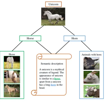
These approaches can be indirectly compared with hu-man being’s inferential mechanism. In fact, ZSL can be addressed by imitating the human being’s mechanism that recognizes a novel category. When finding a novel catego-ry, someone tends to classify it according to the consistence between the visual features and prior knowledge about the unseen classes. For example, as illustrated in Fig. 1, if a child has the prior knowledge of a horse and semantic de-scription of “a unicorn is similar to a horse, apart from a unicorn has a long horn on the head”, the child is very like-ly to accuratelike-ly identify a unicorn the first time it is seen. The mechanism behind this is that the child can imagine a synthesized virtual appearance for a unicorn based on his/her prior knowledge.

Semantic description A unicorn is a mythical creature of legend. The appearance of unicorn is similar to a horse, apart from a unicorn has a long horn in the head.

Horn

Horse Animals with horn

Horse

Unicorn

Figure 1: The mechanism behind human being that recognizes a novel category. Human can identify a unicorn the first time it is seen based on the prior knowledge of a horse and semantic description of “a unicorn is similar to a horse, apart from a unicorn has a long horn in the head”.

In this paper, we also propose a synthesis approach to treat ZSL as a traditional classification task. Based on dic-tionary learning framework, reconstruction of visual fea-tures can be realized with the auxiliary of class prototypes sparsely, and the class-specific properties are preserved. Different with the existing synthesis approaches [6, 19, 20] that synthesize unseen instances with class prototypes, our approach synthesizes the pseudo unseen instances with not only their corresponding class prototypes but also their affinity seen classes.

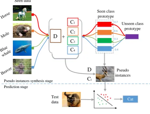
Our approach is referred as Class-Specific Synthesized Dictionary Model (CSSD), which consisits of two stages: 1) Pseudo instances synthesis stage. In this stage, the pro-posed model undergoes two steps. First, it maps the seen class prototypes into a latent space to learn a class-specific encoding matrix for each class, and learns a dictionary matrix simultaneously to reconstruct the visual features within a dictionary learning framework. And then, it syn-thesizes pseudo instances of unseen classes with the class prototypes of affinity seen classes and their correspond-ing encodcorrespond-ing matrices, in which the affinity seen classes represent those seen classes similar to unseen ones. 2) Prediction stage. Classifiers for unseen classes are first trained with these pseudo instances in a supervised way. Afterwards, the labels of test data are predicted by these classifiers. The flowchart of CSSD approach is illustrated in Fig. 2.

In summary, the contributions of our proposed approach can be summarized into two-fold:

• We propose a novel synthesized ZSL approach by syn-thesizing pseudo instances of unseen classes with their corresponding class prototypes and their affinity seen

classes.

• To effectively synthesize unseen pseudo instances, we learn the common properties of all classes as well as the specific properties of each class within a dictionary learning framework. Specifically, it learns both a dic-tionary matrix and a class-specific encoding matrix for each seen class, so as to synthesize pseudo instances for unseen classes with auxiliary of seen class proto-types. In this way, ZSL is transferred to a traditional classification task.

2. Related Work

2.1. Traditional Zero-Shot Learning

The goal of ZSL is to recognize instances from unseen classes. And it is achieved by transferring knowledge from seen classes to unseen ones with a kind of class prototype s-pace. The existing ZSL approaches can be divided into two different strategies, embedding-based ZSL and synthesis-based ZSL.

2.1.1. Embedding-Based ZSL

Embedding-based approaches treat ZSL as a multimodal learning problem that learns the interactions between the visual space and the class prototype space. They are di-vided into three sub-categories in terms of the direction of the embedding function. The first one [12, 17] learns an embedding function to project the visual features to the class prototype space. With the learned function, the test instance can obtain its class embedding vector in the class prototype space. By measuring the semantic similar-ities between the class embedding vector and unseen class prototypes, the test instance is predicted with the nearest neighbor classifier. However, these methods usually suffer from hubness issue [21]. That is, a small number of ob-jects (hubs) may occur as the nearest neighbour of many categories, resulting the diminishing of nearest neighbour method. In order to alleviate this issue, in the approaches of the second sub-category, [13][22] apply an opposite di-rection to map the class prototypes into the visual space. The last sub-category [23, 24, 25] learns a bilinear embed-ding function to project both the visual features and class prototypes into a shared latent space, which can preserve the compatibility scores between different modalities. The correct class usually has a higher score than other class-es. Among these, JEDM [24] is the most related work to ours. The difference between JEDM and CSSD is that our model learns class-specific encoding matrices in terms of different classes while JEDM learns a common encoding matrix for all classes.

2.1.2. Synthesis-Based ZSL

Synthesis-based approaches treat ZSL as a traditional classification task by synthesizing pseudo instances with the unseen class prototypes. The existing approaches differ in the synthesis process. For example, [19] learns manifold

D  C2 3 C

4 C

Seen class prototype

Unseen class prototype

Pseudo instances Seen data

0.4 0.3 0.6 0.7

D

Pseudo instances synthesis stage

Test

data Cat

Prediction stage

1 C

i C

Figure 2: The illustration of our proposed CSSD model for ZSL. In the pseudo instances synthesis stage, it first learns a dictionary matrix D and a class-specific encoding matrix Cifor each seen class

within a dictionary learning framework. Then, pseudo instances for unseen class are synthesized with the help of its affinity seen class-es together with D and Ci. In the prediction stage, classifiers for

unseen classes are first trained with these pseudo instances in a su-pervised way. And then, the labels of test data are predicted by these classifiers.

structure in the class prototype space based on sparse cod-ing and then transfers the manifold information into the visual space to synthesize pseudo instances for predicting the labels of unseen classes. [6, 20] present a diffusion regularization to ensure the balancing distribution of the synthesized data. The proposed CSSD is also a synthesis approach. Different with the existing synthesis approach-es that synthapproach-esize pseudo unseen instancapproach-es only with their corresponding class prototypes, the proposed CSSD syn-thesizes the pseudo instances of unseen classes with both their class prototypes as well as their affinity seen classes.

2.2. Generalized Zero-Shot Learning

The early ZSL work has a limitation that the learned model only can differentiate categories between unseen classes, which violates the reality. Recently, [17, 26] extend ZSL to a more general scene called Generalized Zero-Shot Learning (GZSL), where the test instances are classified into both the seen and unseen classes. [17] designs two novelty detection strategies to differentiate unseen classes from seen classes to help the final object classification. S-ince no training data are available for unseen classes, the learned model tends to classify the test instances into the seen classes. To alleviate this issue, [26] introduces a cali-bration factor to calibrate the classifiers for both seen and unseen classes. And [27] uses a maximum margin frame-work for semantic manifold-based recognition, which con-strains the distance of vocabulary atoms to ensure the la-beled images can be projected closest to their class proto-types than other classes.

Table 1: The notations used in CSSD model.

Notations Description

M number of seen classes

N number of unseen classes

mi number of seen instances ofi-th class

n number of unseen instances

p dimensionality of visual features

q dimensionality of class prototypes Xi∈Rp×mi _{visual features of each seen class}

Xu∈Rp×n visual features of unseen classes

Ai∈Rq×mi _{class prototypes of each seen class}

Au∈Rq×N class prototypes of unseen classes

D dictionary matrix

Ci class-specific encoding matrix ofi-th class Pi class-specific embedding function ofi-th class Q embedding function of all seen classes

ai class prototype ofi-th seen class

aj class prototype ofj-th unseen class

µij class similarities of different classes

xpse_j pseudo instances ofj-th unseen class Apse_j synthesized class prototypes Ppse_i embedding function of selected class

3. The Proposed Model

3.1. Notations

Suppose that we have M seen classes in the train-ing stage and N unseen classes in the testing stage, and each class is associated with a q-dimensional class pro-totype vector in the class propro-totype space. We denote X = [X1,X2,· · · ,XM] as a set ofp-dimensional visual fea-tures fromM seen classes, where Xi∈Rp×mi _{is the visual}

feature set of class i, and mi is the number of seen in-stances of each class. Similarly, Ai ∈ Rq×mi _{is denoted}

as the class prototypes of classi. Let{Xu,Au} denote all the test data, in which Xu∈Rp×n is available only when

predicting the labels. The notations used in this paper are summarized in Table 1.

3.2. Reconstruction of Class-Specific Dictionary Learning Model

The traditional dictionary learning aims at learning a dictionary matrix D to sparsely represent the input data X with its corresponding encoding matrix C. The process is usually followed by an l0 or l1 norm constraint on the

encoding matrix C to make it sparse. The model can be summarized as follows:

{D∗,C∗}=argmin

D,CkX−DCk 2

F+λkCkp+ψ(D,C,X)

(1) where λis a hyper-parameter, and ψ(D,C,X) stands for discriminative functions to ensure the discrimination of D and C.

transfer across different classes, we propose to embed the class prototypes to the dictionary learning model to reveal the relationships between the seen classes and unseen ones. Due to the fact that redundant information exists in the class prototype space, denoting the class prototypes as the encoding matrix C directly will not ensure the sparsity of C. To address this problem, we propose to use an embed-ding function P to map the class prototypes into a latent space, which preserves the semantic relationships between different classes. And the redundant information of the seen class prototypes is decreased when we consider the mapped class prototypes as the encoding matrix. Inspired by this idea, we thus have:

min

P,CkPA−Ck 2

F (2)

where the mapped class prototypes are considered as the encoding matrix C. In this way, there is an advantage that thel0orl1norm constraint on the encoding matrix C can

be removed, and the class prototypes can be embedded into the dictionary-based approach easily to achieve the purpose of knowledge transfer. Therefore, when integrat-ing Eq. (2) into the dictionary learnintegrat-ing framework, we have an objective function as follows:

{P∗,D∗,C∗}=arg min

P,D,CkX−DCk 2

F+kPA−Ck

2 F

+ψ(D,P,C,X,A)

(3)

The first term in Eq. (3) is used to jointly reconstruct the visual features of seen classes with the linear combination between the dictionary matrix D and the mapped class prototypes C in the latent space. The second term is to map class prototypes into a latent space of seen classes and unseen classes to realize knowledge transfer. And the last term ψ(D,P,C,X,A) is a discriminative term to achieve other constraints.

However, due to the different distribution of each class, a global linear model is oversimple to represent complicated relationships between visual features and class prototypes of all seen classes. And a nonlinear model is easily overfit-ting on the seen classes. Thus, we prefer to learn a unique linear model for each class to better reflect their relation-ships. Based on this idea, instead of learning a common encoding matrix, we propose to learn a class-specific en-coding matrix for each seen class to preserve discriminative information. Thus, the objective function becomes:

min

D,C_i,P_i,Q M

X

i=1

kXi−DCik

2

F +kPiAi−Cik 2 F

+λkQA_i−Cik 2

F+γkPik 2

F+kQk

2 F,kdik

2 2≤1

(4) The first term in Eq. (4) represents the reconstruction error in terms of different classes. D is the dictionary ma-trix shared by all seen classes, Ci and Xi represent the class-specific encoding matrix and visual features of each seen class, respectively. The second and third terms are

the process of mapping class prototypes into a latent s-pace, and the difference between them locates that the for-mer distinguishes the discriminative information between different classes and the latter preserves the same parts. That is, Pi(1≤i≤M) is thought to be the class-specific embedding function of each seen class, and Q is consid-ered to be an embedding function shared by all different seen classes. Andλis a hyper-parameter to trade off the proportion between them, which is determined through a cross-validation strategy. The last two terms are regu-larizers, whereγ is another hyper-parameter. Besides, di denotes thei-th atom of the dictionary matrix D. Utilizing

l2 norm to constrain the value of the atom of dictionary

matrix D is to make their distribution more balanced so as to make sure the model more stable.

Next, we introduce the optimization approach. When solving D, Ci, Pi and Q simultaneously, Eq. (4) is not a convex objective function while it is convex for solving each variable separately. The optimization can be done according to the following steps.

(1) Fix D, Pi and Q, and update Ci

C∗_i =argmin

Ci

M

X

i=1

kXi−DCik

2

F+kPiAi−Cik 2 F

+λkQAi−Cik 2 F

(5)

This is a standard least squares problem which can get its closed-form solution when we take the derivative of Eq. (5) with respect to Ci and make it equal to zero:

C∗_i = DTD + (1 +λ) I−1

(DXi+ (Pi+λQ) Ai) (6)

(2) Fix D and Ci, update Piand Q



  

  

P∗

i =argmin

Pi

M

P

i=1

kPiAi−Cik

2

F+γkPik 2 F

Q∗=argmin

Q M

P

i=1

λkQA_i−Cik2_F+kQk2_F

(7)

Due to Pi and Q are independent, we can obtain their closed-form solutions respectively, which are as follows:



 

 

P∗_i = CiATi

AiATi +γI

−1

Q∗=

_M

P

i=1

λCiATi

M

P

i=1

λAiATi + I

−1 ₍₈₎

(3) Fix Ci, Pi and Q , update D

D∗=argmin

D M

X

i=1

kXi−DCik

2 F,kdik

2

2≤1 (9)

The optimization of D can be achieved by introducing an intermediate variable S :

D∗=argmin

D,S M

X

i=1

kXi−DCik

2

F, s.t.D = S, ksik

2 2≤1

(10)

Similarities of visual features

grizzly bearkiller whale beaver

dalmatian horse

german shepherd blue whalesiamese cat

skunk mole

(a)

0.3839 0.4339 0.36 0.3114 0.3885 0.4381 0.4311 0.5614 0.6856 0.8357 0.533 0.626 0.3 0.285 0.4371 0.5697 0.3618 0.4866 0.4147 0.5452

Similarities of class prototypes

mole

grizzly bearkiller whale beaver

dalmatian horse

german shepherp blue whalesiamese cat

skunk

(b)

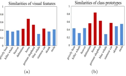
Figure 3: The consistency of similarities between visual features and class prototypes. In both sub-figures, the height of each column is the similarity between each class and “antelope”. And the red columns correspond to affinity classes of “antelope”.

The solution to Eq. (10) can be obtained by ADMM al-gorithm. When the difference between two adjacent iter-ations is less than a threshold, the optimization process stops.

3.3. Synthesis of Pseudo Instances

Most existing approaches directly utilize the model learned from seen classes to predict the labels of unseen classes [28, 29, 30]. However, since the distribution of seen classes and unseen ones are different, the model learned from seen classes cannot be well generalized to unseen ones. To diminish this distribution gap, we propose to use the combination of affinity seen classes to replace unseen classes to train classifiers. We have the following assump-tion.

Assumption The semantic similarities among

class-es obtained with visual featurclass-es are consistent with those obtained with class prototypes. Thus, the combination of affinity seen classes prototypes with the embedding model can approximate the visual features of unseen classes.

To verify the correctness of our assumption, we perform statistical studies on AwA dataset. Take the class “ante-lope” for example. As illustrated in Fig. 3, we can find that the similarities between the class “antelope” and the other ten classes with visual prototypes (i.e., the mean vi-sual features of each class) are similar with those obtained with the class prototypes (i.e., class attributes). Specifical-ly, “horse”, “german shepherd”, “siamese cat” and “dal-matian” are more similar than the others, such as “blue whale” in visual space (i.e., Fig.3 (a)). And this close-ness are kept in the class prototype space (i.e., Fig.3 (b)). Thus, it verifies the consistency of similarities between vi-sual features and class prototypes.

Based on this assumption, the pseudo instances of un-seen classes can be synthesized with their most affinity un-seen classes. Therefore, the j-th pseudo instancesxpse_j can be synthesized with the following form:

xpse_j =

k

X

i=1

µijD Pseli +λQ

aj,(1≤j≤N) (11)

wherekdenotes the number of selected affinity seen class-es, Psel

i is the embedding function corresponding to the

i-th selected class, and µij is the class similarity that is considered as the weight of each affinity class.

There are many possible ways to evaluate the similari-ties between different classes, such as cosine distance, Eu-clidean distance, and so on. In this work, we use cosine dis-tance to measure the similarities between different classes

µij=

hai, aji

kaik₂kajk₂

(12)

where ai and aj are the class prototypes of the i-th seen class and thej-th unseen class.

We utilize SVM as the classifiers. Since enough labeled data are required to train SVM classifiers, we have to pre-pare several class prototypes for each unseen class in ad-vance to synthesize enough pseudo instances.

In the visual space, data from different classes are sepa-rated and form a tight cluster. Thus we assume each class follows a Gaussian distribution. Considering the similari-ties among different classes in visual space are consistent with those in class prototype space, the prepared class pro-totypes Apse_j should also follow a Gaussian distribution

Apse_j =aj+δ·I (13)

whereajserves as the mean value of Gaussian distribution andδis the variance. Therefore, we are able to synthesize plenty of unseen class prototypes for the same class, which ensures the diversity of synthesized pseudo instances.

Algorithm 1 summarizes the process of our CSSD model.

4. Experiments

4.1. Datasets and Settings

In this section, we conduct extensive experiments on four benchmark datasets to illustrate the effectiveness and superiority of our proposed model. The four datasets are Animals with Attributes (AwA) [18], Caltech-UCSD Bird2011 (CUB) [31], aPascal-aYahoo (aPY) [7], and SUN Attribute (SUN) [32]. Table 2 summarizes the details of the four datasets.

Visual features. To compare fairly with the existing

approaches, we use the VGG-19 [33] deep features extract-ed from popular CNN architecture as the visual features.

Class prototypes. In this paper, we choose both

at-tributes and Word2Vec as the class prototypes for AwA and CUB datasets, respectively. The attributes are pre-defined and Word2Vec are obtained by a large text corpus based on a neural language processing technology. For aPY and SUN datasets, we only use attributes as the class prototypes since few competitors are evaluated with Word2Vec on them.

Implementation details. In our proposed model,

Algorithm 1: The process of CSSD Input:

1: The seen domain:

Visual features of each seen class Xi∈Rp×mi_;

Class prototypes of each seen class Ai∈Rq×mi

Hyper-parameterλ,γ; 2: The unseen domain:

Visual features of unseen classes Xu∈Rp×n;

Class prototypes of unseen classes Au∈Rq×N;

Parameterσ,k;

Output: The predicted labels of test data. Training:

3: Repeat;

4: Update Ci according to Eq. (6); 5: Update Pi and Q according to Eq. (8); 6: Update D according to Eq. (10); 7: Until the iteration stops;

8: Return Pi, Q and D; Synthesizing data:

9: Synthesize class prototypes of each unseen classes Apse_j according to Eq. (13);

10: Compute class similarities µij according to Eq. (12); 11: Synthesize pseudo instancesxpse_j with affinity seen

classes according to Eq. (11); Testing:

12: Train SVM classifiers with the pseudo instancesxpse_j ; 13: Predict the labels of test data with the trained SVM

classifiers.

Table 2: The statistics of the four datasets used in the experiments. ’/’ in columns of ’Instances’ and ’Classes’ represents the split of train-ing/test instances and seen/unseen classes, respectively.

Dataset Instances Attribute Classes

AwA 24,295/6,180 85 40/10

CUB 8,855/2,933 312 150/50

aPY 12,695/2,644 64 20/12

SUN 14,140/200 102 707/10

training stage, and σ serves as the variance of the Gaus-sian distribution, andk is the number of selected affinity seen classes. We use 5-fold crosvalidation strategy to s-elect the parameters with the best performance. That is, we split the training data into five parts, one for validation and the rest as the training set. Once the parameters are fixed, all seen instances form the training set to get the final model.

4.2. Comparative Results of Traditional ZSL

The performance of Traditional ZSL mainly indicates the transferability from seen classes to unseen ones of the ZSL approaches. In this part, we conduct Traditional ZSL experiments with both the attributes and Word2Vec.

First, we select seven attribute-based approaches for comparison, including 1) Convex Combination of Semantic Embedding (ConSE) [12], 2) Matrix tri-Factorization with

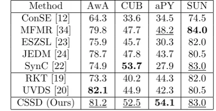
Table 3: Traditional ZSL results (%) of different approaches on four datasets with attributes. For each column, the best one is marked in bold and the second best one is marked with underline.

Method AwA CUB aPY SUN

ConSE [12] 64.3 33.6 34.5 74.5

MFMR [34] 79.8 47.7 48.2 84.0

ESZSL [23] 75.9 45.7 30.3 82.0

JEDM [24] 78.7 47.8 43.7 80.5

SynC [22] 74.9 53.7 27.9 83.0

RKT [19] 73.3 40.2 44.3 82.0

UVDS [20] 82.1 44.9 42.3 80.5

CSSD (Ours) 81.2 52.5 54.1 83.0

Table 4: Traditional ZSL results (%) of different approaches on AwA and CUB datasets with Word2Vec. For each column, the best one is marked in bold and the second best one is marked with underline.

Method AwA CUB

ConSE [12] 50.5 30.7

ESZSL [23] 67.5 30.6

JEDM [24] 72.4 31.2

SynC [22] 67.3 30.9

RKT [19] 76.9 28.9

UVDS [20] 62.9 32.1

CSSD (Ours) 72.7 32.9

Manifold Regularizations (MFMR) [34], 3) Embarrassing-ly Simple Approach to Zero-Shot Learning (ESZSL) [23], 4) Joint Embedding Dictionary Model (JEDM) [24], 5) Synthesized Classifiers for Zero-Shot Learning (SynC) [22], 6) Relational Knowledge Transfer for Zero-Shot Learning (RKT) [19], and 7) Zero-shot Learning Using Synthesised Unseen Visual Data with Diffusion Regularisation (UVDS) [20]. Specifically, the first five approaches are embedding-based approaches, and the last two are synthesis-embedding-based approaches.

The comparison results are shown in Table 3. The re-sults of MFMR [34] and UVDS [20] are cited directly from their published papers and the performances of the rest competitors are obtained with the released codes using the same features as our CSSD. We report their best per-formances after tuning parameters. The parameters are selected from{0.001,0.01,0.1,1,10,100,1000}.

As illustrated in Table 3, we observe that the proposed CSSD achieves state-of-the-art performances. Specifically, except the MFMR [34] and SynC [22], our CSSD is bet-ter than the other embedding-based approaches, indicat-ing that CSSD learns a more effective embeddindicat-ing function by learning common properties of all classes and specific properties of each class within a dictionary learning frame-work simultaneously. Unlike the other embedding-based approaches that learn an embeding function directly, SynC [22] builds a weighted graph with pseudo class prototypes in the class prototype space, and constructs synthesized classifiers in the visual space, achieving best result on the CUB dataset. Compared with synthesis-based ones, CSSD achieves best performances on three datasets except AwA,

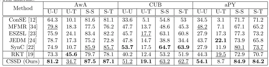
Table 5: Generalized ZSL results (%) of different approaches. For each column, the best one is marked in bold and the second best one is marked with underline.

Method AwA CUB aPY

U-U U-T S-S S-T U-U U-T S-S S-T U-U U-T S-S S-T

ConSE [12] 64.3 10.1 81.6 81.1 33.6 5.1 54.8 53 34.5 3.1 71.7 71.2

MFMR [34] 79.8 18.3 77.5 76.2 47.7 13.7 48.6 45.3 48.2 7.1 67.1 65.2

ESZSL [23] 75.9 24.1 83.4 82.2 45.7 17.7 63.1 60.8 27.9 17.3 77.3 73.2

JEDM [24] 78.7 17.3 75.2 72.8 47.8 14.7 38.8 34.4 43.7 22.1 73.9 65.8

SynC [22] 74.9 10.7 85.9 85.7 53.7 17.5 64.7 63.9 27.9 11.9 80.1 73.7

RKT [19] 73.3 45.6 79.7 78.1 40.2 12.4 53.2 51.9 44.3 19.5 72.9 70.7

CSSD (Ours) 81.2 34.7 87.5 87.1 51.2 19.1 63.2 62.7 54.1 8.7 84.9 84.2

on which CSSD is only 0.9% lower than UVDS [20]. Since CSSD synthesizes pseudo instances with affinity seen class-es and lacks the consideration of the balanced distribution on each dimension.

Next, we select Word2Vec as the class prototypes and conduct experiments on the same approaches except MFMR [34] since no performance is available in the orig-inal paper. The performances of different approaches are summarized in Table 4. From the results, we can find that our model outperforms all the embedding-based approach-es. Besides, CSSD beats UVDS [20] but is inferior than RKT [19] on AwA dataset. This is may be that different kinds of class prototypes have different effects.

4.3. Comparative Results of Generalized ZSL

Compared with Traditional ZSL, Generalized ZSL eval-uates not only the transferability from seen classes to un-seen ones but also the discriminability across both the un-seen and unseen classes. In this part, we conduct a set of ex-periments on AwA, CUB, and aPY datasets under the Generalized ZSL setting.

There are four evaluation scenarios under the General-ized ZSL setting, including U-U, U-T, S-S, and S-T. Specif-ically, U-U is the same as the setting of Traditional ZSL, which means classifying test data from unseen classes in-to the candidate unseen classes. U-T means classifying the test data from unseen classes into the joint space of seen classes and unseen ones. While S-S is the setting of multi-class classification actually, which means the test da-ta are from seen classes and the candidate classes are the seen classes as well, and S-T is a scenario that classifies the test data from seen classes into the joint space. For S-S, we randomly select 20% of the seen instances to be the test data, and the remaining seen instances are used to train the model. While for S-T, we also select 20% of the instances from seen classes and merge them with the instances from unseen classes to compose the test data.

We select six attribute-based approaches for compari-son. Table 5 summarizes the best results of different mod-els, the parameters of which are fine tuned by ourselves using the codes released in the original papers. From the results, we observe that the performances of S-T are close to those of S-S, indicating that most of the test data from

seen classes are classified correctly. However, the perfor-mances of U-T decrease more obviously than those of U-U, indicating that CSSD is less discriminative to distinguish differences between seen classes and unseen ones. These observations illustrate that the Generalized ZSL is a more challenging task than Traditional ZSL. On AwA dataset, compared with embedding-based approaches, our model achieves best performances under four different scenarios, which obtains an improvement of 1.4%, 10.6%, 0.6% and 1.5% over the second best approach, respectively. On aPY dataset, we also achieve the best performances except for U-T. The reason locates that the aPY dataset is a coarse-grained dataset where classes share little information with each other, resulting that the class-specific encoding matri-ces learn ineffective discriminative information. For CUB dataset, the performances of our CSSD achieve the best performance on U-T, and the second-best performance on the other scenarios. While considering the discriminability of the pseudo instances, we can find the performances of CSSD are lower than RKT [19] on AwA and aPY dataset-s. This is because the synthesis process of CSSD pre-serves more transferable information other than discrim-inative information on coarse-grained datasets compared with RKT [19]. Specifically, the discriminability of at-tributes on coarse-grained dataset is higher than that on fine-grained dataset. Compared with RKT [19] which thesizes pseudo instances with all seen classes, CSSD syn-thesizes pseudo instances only with affinity seen classes and ignores dissimilar classes, and this method makes C-SSD less discriminability than RKT.

4.4. Parameter Sensitivity Analysis

There are two hyper-parameters in the training stage, and a parameter in the process of synthesizing pseudo vi-sual features. λ is the hyper-parameter to trade-off the weight of the same parts and discriminative parts between different classes, and γ is the balance parameter of reg-ularizer. Besides, kis the number of the selected affinity seen classes. To evaluate their influences, we conduct a list of experiments on AwA and CUB datasets. In the exper-iments, we change one parameter while fixing the others with their best values.

70 72 74 76 78 80 82

0.001 0.01 0.1 1 10 100 1000

Accuracy

(%)

AwA

 

(a)

20 25 30 35 40 45 50 55

0.001 0.01 0.1 1 10 100 1000

Accuracy

(%)

CUB

 

(b)

Figure 4: The influences of different λon AwA and CUB datasets with attributes and Word2Vec, respectively. AndAandWare short for attributes and Word2Vec.

67 69 71 73 75 77 79 81 83

0.001 0.01 0.1 1 10 100 1000

Accuracy

(%)

AwA

 

(a)

20 25 30 35 40 45 50 55

0.001 0.01 0.1 1 10 100 1000

Accuracy

(%)

CUB

 

(b)

Figure 5: The influences of different γon AwA and CUB datasets with attributes and Word2Vec, respectively. AndAandWare short for attributes and Word2Vec.

datasets. The curves in Fig.4 (a) show that the perfor-mances initially increase with the increase ofλand achieve their peaks, and then decline on the AwA dataset. The performances achieve their best value when λ is equal to 0.01, illustrating that although the discriminative infor-mation plays a more important role than the same parts among different classes, preserving the information of same parts is also necessary. On CUB dataset, the overall trends are similar with Fig.4 (a), while the curses achieve their peaks when λ is equal to 1. We report the performances with their best value on the peak.

Two sub-figures in Fig. 5 show the effects of differentγ

on both datasets. The performances are robust with the increase ofγon the AwA dataset with both attributes and Word2Vec. When the value is larger than 10, the curves begin fluctuating slightly. On CUB dataset, the trends of curves are similar with that of AwA dataset, revealing the insensitivity ofγ.

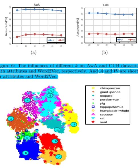
When evaluating the influence of parameterk, its range should be set in advance according to the number of seen classes. Specifically, we set it is{5,10,15,20,25,30}on AwA dataset and {20,30,40,50,60,70} on CUB dataset, respec-tively. Fig. 6 shows the trend of the accuracy curves with the increase of k on both datasets. And we can observe that the two curves ofAandWhave the similar trend, i.e., rise or fall almost at the same number on both datasets. On AwA dataset, the accuracy reaches maximum when

k is equal to 15, whereas on CUB dataset the number is 30. The reason behind this phenomenon is that the

70 72 74 76 78 80 82

5 10 15 20 25 30

Accu

racy(

%)

AwA

 

(a)

25 30 35 40 45 50 55

20 30 40 50 60 70

Accur

acy(

%

)

CUB

 

(b)

Figure 6: The influences of differentkon AwA and CUB datasets with attributes and Word2Vec, respectively. AndAandWare short for attributes and Word2Vec.

−50 0 50

−40 −30 −20 −10 0 10 20 30 40

1 2

3 4

5

6

7 8

9

10

chimpanzee giant+panda leopard persian+cat pig hippopotamus humpback+whale raccoon rat seal

Figure 7: t-SNE visualization for our synthesized pseudo instances on AwA dataset.

coarse-grained AwA dataset has fewer similar categories than that of fine-grained CUB dataset.

4.5. Further Analysis

With the learned model, the pseudo instances of un-seen classes are synthesized with class prototypes of their affinity seen classes and their corresponding class-specific encoding matrices. Given the unseen class prototype, we consider it as the mean value of the Gaussian distribution, while the variance is determined by 5-fold cross-validation. We select the best value of σ to visualize them with t-SNE approach, as illustrated in Fig. 7. It can be observed that the pseudo instances from the same class are gathered around their corresponding class prototypes. Although each cluster of pseudo instances has a little overlap, the pseudo instances are enough to form separate clusters for the ten unseen classes, showing that the proposed CSSD approach can effectively reveal the visual distribution of the unseen classes.

5. Conclusion

In this paper, we proposed a novel approach for ZSL by synthesizing pseudo instances for unseen classes within a dictionary learning framework. It learns a dictionary matrix and a class-specific encoding matrix for each seen class to connect the interactions between the visual space

and the class prototype space. The distribution of unseen classes is then synthesized with their affinity seen classes using the learned model. The experimental results on four benchmark datasets illustrate that the proposed CSSD approach achieves the state-of-the-art performances on both Traditional ZSL and Generalized ZSL tasks.

Acknowledgments

This work was supported by the National Natural Science Foundation of China under Grants 61771329, 61472273, and 61632018.

References

[1] X. Li, M. Fang, J. Wu, Zero-shot classification by transferring knowledge and preserving data structure, Neurocomputing 238 (2017) 76–83.

[2] Y. Yu, Z. Ji, J. Guo, Y. Pang, Zero-shot learning with regular-ized cross-modality ranking, Neurocomputing 259 (2017) 14–20. [3] M. Liu, D. Zhang, S. Chen, Attribute relation learning for

zero-shot classification, Neurocomputing 139 (2014) 34–46. [4] M. Elhoseiny, B. Saleh, A. Elgammal, Write a classifier:

Zero-shot learning using purely textual descriptions, in: IEEE Inter-national Conference on Computer Vision, 2014, pp. 2584–2591. [5] Y. Li, D. Wang, H. Hu, Y. Lin, Y. Zhuang, Zero-shot recognition using dual visual-semantic mapping paths, in: IEEE Conference on Computer Vision and Pattern Recognition, 2017, pp. 5207– 5215.

[6] Y. Long, L. Liu, L. Shao, F. Shen, G. Ding, J. Han, From zero-shot learning to conventional supervised classification: Unseen visual data synthesis, in: IEEE Conference on Computer Vision and Pattern Recognition, 2017, pp. 6165–6174.

[7] A. Farhadi, I. Endres, D. Hoiem, D. Forsyth, Describing objects by their attributes, in: IEEE Conference on Computer Vision and Pattern Recognition, 2009, pp. 1778–1785.

[8] C. H. Lampert, H. Nickisch, S. Harmeling, Attribute-based clas-sification for zero-shot visual object categorization, IEEE Trans-actions on Pattern Analysis and Machine Intelligence 36 (3) (2014) 453–465.

[9] S. J. Hwang, F. Sha, K. Grauman, Sharing features between objects and their attributes., in: IEEE Conference on Computer Vision and Pattern Recognition, 2011, pp. 1761–1768. [10] T. Mikolov, I. Sutskever, K. Chen, G. Corrado, J. Dean,

Dis-tributed representations of words and phrases and their compo-sitionality, Advances in Neural Information Processing Systems 26 (2013) 3111–3119.

[11] J. Pennington, R. Socher, C. Manning, Glove: Global vectors for word representation, in: Conference on Empirical Methods in Natural Language Processing, 2014, pp. 1532–1543. [12] M. Norouzi, T. Mikolov, S. Bengio, Y. Singer, J. Shlens,

A. Frome, G. S. Corrado, J. Dean, Zero-shot learning by convex combination of semantic embeddings, in: International Confer-ence on Learning Representations, 2014, pp. 1–9.

[13] Y. Shigeto, I. Suzuki, K. Hara, M. Shimbo, Y. Matsumoto, Ridge regression, hubness, and zero-shot learning, in: The Eu-ropean Conference on Machine Learning and Knowledge Dis-covery in Databases, 2015, pp. 135–151.

[14] Z. Ji, Y. Xie, Y. Pang, L. Chen, Z. Zhang, Zero-shot learning with multi-battery factor analysis, Signal Processing 138 (2017) 265–272.

[15] A. Frome, G. S. Corrado, J. Shlens, S. Bengio, J. Dean, T. Mikolov, et al., Devise: A deep visual-semantic embedding model, in: Advances in Neural Information Processing Systems, 2013, pp. 2121–2129.

[16] Y. Fu, T. M. Hospedales, T. Xiang, Z. Fu, S. Gong, Transduc-tive multi-view embedding for zero-shot recognition and

anno-tation, in: European Conference on Computer Vision, 2014, pp. 584–599.

[17] R. Socher, M. Ganjoo, C. D. Manning, A. Ng, Zero-shot learning through cross-modal transfer, in: Advances in Neural Informa-tion Processing Systems, 2013, pp. 935–943.

[18] C. H. Lampert, H. Nickisch, S. Harmeling, Learning to detect unseen object classes by between-class attribute transfer, in: IEEE Conference on Computer Vision and Pattern Recognition, 2009, pp. 951–958.

[19] D. Wang, Y. Li, Y. Lin, Y. Zhuang, Relational knowledge trans-fer for zero-shot learning., in: AAAI, 2016, pp. 2145–2151. [20] Y. Long, L. Liu, F. Shen, L. Shao, X. Li, Zero-shot learning

us-ing synthesised unseen visual data with diffusion regularisation, IEEE Transactions on Pattern Analysis and Machine Intelli-gence (2018) 1–14.

[21] A. Lazaridou, G. Dinu, M. Baroni, Hubness and pollution: Delving into cross-space mapping for zero-shot learning, in: Meeting of the Association for Computational Linguistics and the International Joint Conference on Natural Language Pro-cessing, 2015, pp. 270–280.

[22] S. Changpinyo, W. L. Chao, B. Gong, F. Sha, Synthesized clas-sifiers for zero-shot learning, in: IEEE Conference on Computer Vision and Pattern Recognition, 2016, pp. 5327–5336. [23] B. Romera-Paredes, P. H. S. Torr, An embarrassingly simple

approach to zero-shot learning, in: International Conference on International Conference on Machine Learning, 2015, pp. 2152– 2161.

[24] Y. Yu, Z. Ji, X. Li, J. Guo, Z. Zhang, H. Ling, F. Wu, Transduc-tive zero-shot learning with a self-training dictionary approach, IEEE Transactions on Cybernetics (2018) 1–12.

[25] Z. Akata, S. Reed, D. Walter, H. Lee, B. Schiele, Evaluation of output embeddings for fine-grained image classification, in: IEEE Conference on Computer Vision and Pattern Recognition, 2015, pp. 2927–2936.

[26] W. L. Chao, S. Changpinyo, B. Gong, F. Sha, An empirical study and analysis of generalized zero-shot learning for object recognition in the wild, in: European Conference on Computer Vision, 2016, pp. 52–68.

[27] Y. Fu, L. Sigal, Semi-supervised vocabulary-informed learning, in: IEEE Conference on Computer Vision and Pattern Recog-nition, 2016, pp. 5337–5346.

[28] Z. Akata, F. Perronnin, Z. Harchaoui, C. Schmid, Label-embedding for attribute-based classification, in: IEEE Confer-ence on Computer Vision and Pattern Recognition, 2013, pp. 819–826.

[29] Y. Xian, Z. Akata, G. Sharma, Q. Nguyen, M. Hein, B. Schiele, Latent embeddings for zero-shot classification, in: IEEE Con-ference on Computer Vision and Pattern Recognition, 2016, pp. 69–77.

[30] R. Qiao, L. Liu, C. Shen, A. V. D. Hengel, Less is more: zero-shot learning from online textual documents with noise suppres-sion, in: IEEE Conference on Computer Vision and Pattern Recognition, 2016, pp. 2249–2257.

[31] C. Wah, S. Branson, P. Welinder, P. Perona, S. Belongie, The caltech-ucsd birds200-2011 dataset, California Institute of Tech-nology.

[32] G. Patterson, C. Xu, H. Su, J. Hays, The sun attribute database: Beyond categories for deeper scene understanding, International Journal of Computer Vision 108 (1-2) (2014) 59– 81.

[33] K. Simonyan, A. Zisserman, Very deep convolutional networks for large-scale image recognition, in: International Conference on Learning Representations, 2014.