high dimensional time-series
Lawrence Bardwell, B.Sc.(Hons.), M.Res
Submitted for the degree of Doctor of Philosophy
at Lancaster University.
This thesis looks at developing efficient methodology for analysing high dimensional time-series, with an aim of detecting structural changes in the properties of the time series that may affect only a subset of dimensions.
Firstly, we develop a Bayesian approach to analysing multiple time-series with the aim of detecting abnormal regions. These are regions where the properties of the data change from some normal or baseline behaviour. We allow for the possibility that such changes will only be present in a, potentially small, subset of the time-series. A motivating application for this problem comes from detecting copy number variation (CNVs) in genetics, using data from multiple individuals.
Secondly, we present a novel approach to detect sets of most recent changepoints in panel data which aims to pool information across time-series, so that we preferentially infer a most recent change at the same time point in multiple series.
Lastly, an approach to fit a sequence of piece-wise linear segments to a univariate time series is considered. Two additional constraints on the resulting segmentation are imposed which are practically useful: (i) we require that the segmentation is robust to the presence of outliers; (ii) that there is an enforcement of continuity between the linear segments at the
First and foremost I would like to thank my supervisors, Idris Eckley and Paul Fearnhead. It has been an honour and privilege to have worked with such fine researchers (and people) over the past few years. I am very grateful for all the time and effort they have spent on my project whilst showing unbounded patience and knowledge.
I am very grateful for the financial support provided by the EPSRC and BT. I would like to thank my industrial supervisor Martin Spott for all the helpful conversations, guidance and making my visits to BT very useful and enjoyable.
Thanks also to all the staff and students at the STOR-i Centre for Doctoral Training for providing such an enjoyable working environment of which I am very lucky to have been part of. Jonathan Tawn deserves a special thank you for always going above and beyond for everyone at STOR-i.
Finally, to my family and Kirsti, whose continual support, encouragement and love through-out this process helped me get through it relatively unscathed, words cannot express how grateful I am.
I declare that the work in this thesis has been done by myself and has not been submitted elsewhere for the award of any other degree.
Lawrence Bardwell
Chapter 4 has been accepted for publication as Bardwell, L., and Fearnhead, P. (2017). Bayesian Detection of Abnormal Segments in Multiple Time Series. Bayesian Analysis.
Chapter 5 has been submitted toTechnometrics as Bardwell, L., Eckley, I., Fearnhead, P., Smith, S., and Spott, M. (2017). Most recent changepoint detection in Panel data.
Abstract I
Acknowledgements III
Declaration IV
Contents VIII
List of Figures XIII
List of Tables XVIII
1 Introduction 1
1.1 Telecommunications event data . . . 2 1.2 Thesis structure . . . 3
2 Changepoint detection for univariate time series 6
2.1 Notation . . . 7 2.2 Optimisation methods for changepoint detection . . . 8
2.2.1 Segment Neighbourhood . . . 11
2.2.2 Optimal Partitioning . . . 12
2.2.3 Pruning . . . 14
2.2.4 Penalty . . . 22
2.2.5 Binary Segmentation . . . 24
2.3 Bayesian inference for changepoint models . . . 26
2.3.1 Exact online inference . . . 29
2.3.2 Approximate filtering . . . 33
3 Changepoint detection for Multivariate time series 37 3.1 Full change model . . . 39
3.2 Subset change model . . . 40
4 Bayesian detection of abnormal segments in multiple time series 45 4.1 Introduction . . . 45
4.2 The Model . . . 49
4.2.1 Hidden State Model . . . 50
4.2.2 Likelihood model . . . 53
4.3 Inference . . . 57
4.3.1 Exact On-line inference . . . 57
4.3.2 Approximate Inference . . . 58
4.3.4 Hyper-parameters . . . 60
4.3.5 Estimating a Segmentation . . . 61
4.4 Asymptotic Consistency . . . 62
4.5 Results . . . 66
4.5.1 Simulated Data from the Model . . . 68
4.5.2 Simulated CNV Data . . . 71
4.5.3 Analysis of CNV Data . . . 76
4.6 Discussion . . . 80
5 Most recent changepoint detection in Panel data 82 5.1 Introduction . . . 82
5.2 A Penalised Cost Approach to Most Recent Changepoint Detection . . . 87
5.2.1 Analysing a Univariate Time Series . . . 87
5.2.2 Extension to panel data . . . 90
5.3 Optimal set of most recent changepoints . . . 92
5.4 Simulation study . . . 96
5.5 Applications . . . 105
5.5.1 Telecommunications event data . . . 106
5.5.2 Corporate finance data . . . 109
5.6 Discussion . . . 114
out-liers 116
6.1 Introduction . . . 116
6.2 Problem set-up . . . 121
6.3 Algorithms . . . 124
6.3.1 Change in regression . . . 124
6.3.2 Change in slope . . . 126
6.4 Simulation study . . . 135
6.4.1 Performance of different segmentation methods . . . 135
6.5 Telecommunications event data . . . 140
6.6 Discussion . . . 141
7 Conclusions and future work 143 7.1 Future work . . . 144
7.1.1 Higher dimensional parameters in the BARD method . . . 145
7.1.2 Modelling dependence . . . 147
A Lemmas for Proof of Theorem 4.4.1 149 A.1 Lemmas for Proof of Theorem 4.4.2 . . . 156
B Updating the polynomials 161
1.1.1 The number of events that occur per week over the entire telecommunications network measured over a three and a half year time period (175 weeks). . . . 2 1.1.2 A grid showing all possible combinations of Regions and Event types and the
number of events that occur per week for the combination considered. . . 3
2.1.1 Three time series having a single change. A mean change on the left, variance change in the middle and change in regression on the right. . . 8 2.2.1 A time series of length 1000 with the changepoints found using the OP/PELT
methods highlighted in red. . . 18 2.2.2 The number of candidate changepoints at each time pointt for OP (in black)
and PELT (in red). The vertical dashed lines give the location of the change-points found (identical for both methods). . . 18
3.0.1 A multivariate series with three dimensions where any changes that occur affect all three series at the same time. We call this the full change model. . 38
3.0.2 A multivariate series with three dimensions where the changes that occur only affect a subset of the three series at each changepoint. We call this the subset change model. . . 39 3.0.3 A multivariate series with three dimensions where any changes that occur
affect all three series but at slightly different times. We call this the lagged change model. . . 39
4.1.1 Log-R ratios from 6 individuals for a small portion of chromosome 16. We indicate the baseline level (mean zero) by a horizontal line in blue and the identified CNV (abnormal region) is highlighted between two vertical black lines with the mean of the affected individuals in red. . . 47 4.5.1 Empirical distribution of features of the optimal segmentation of CNV data
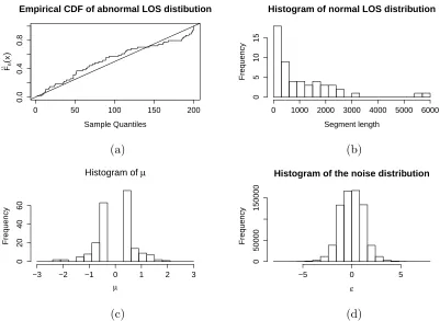
obtained using the PASS method. (a) QQ-plot of length (measured in num-ber of observations) of abnormal segments against a Uniform distribution on {1,2, . . . ,200}; (b) histogram of length (measured in number of observations) of normal segments; (c) histogram of estimated mean for abnormal segments; and (d) histogram of residuals. . . 73 4.5.2 All the time pointstfor which the posterior probability lies in a certain interval
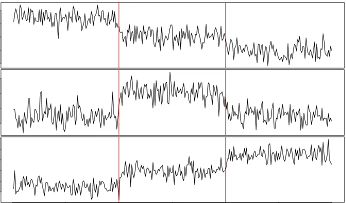
5.1.1 An example of six of the event count time-series. These show different patterns. The left-hand column has two series consistent with a constant positive trend since around week 40. The middle column show series with evidence for a recent increase in trend around week 140. The right-hand column shows series with evidence for a decrease in the rate of events from around week 160. In each case we show our estimate of the most recent changepoint – see Section 5.5.1 for more detail. . . 83 5.4.1 The computational cost when we changed the maximum number of most recent
changepoints to search for. . . 105 5.5.1 The aggregate series segmented into piece wise linear regressions. . . 107 5.5.2 The aggregate series for each of the five groups of series. Their respective
6.1.1 Four plots showing the different data models we consider in this paper. These include data with or without outliers and an underlying process which is con-tinuous or non-concon-tinuous at the changepoints. In each figure we show the true segmentation of the data in red and the standard estimated segmentation under the assumption of Normally distributed residuals (the OLS segmenta-tion) in blue. The standard OLS method works reasonably well for situations with no outliers (Figures 6.1.1a and 6.1.1c). However, for data with outliers (Figures 6.1.1b and 6.1.1d) the standard estimation method is heavily affected. This can be seen from the large deviations from the red and blue lines and the spikes in the blue line at outlier locations. The two figures in the top row show examples of the piece-wise change in regression model whereas the bottom row shows the change in slope model (Figures 6.1.1c and 6.1.1d). The underlying data generating process for the change in slope model is continuous at the changepoints. . . 119 6.3.1 A time series on the left with changepoints shown in red with outliers
high-lighted as thicker black circles. On the right a plot of the (logarithm of the) number of quadratics considered at each time step for the inequality pruning method in black and with no pruning in blue. . . 131 6.3.2 A time series on the left with changepoints shown in red with outliers
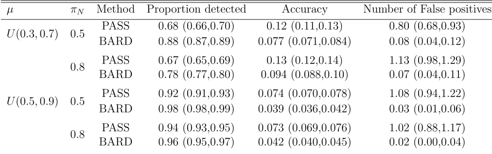
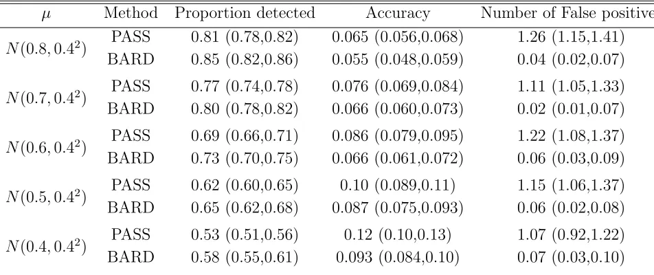
4.5.1 Scenarios differed in the prior for µ and the value ofπN used to simulate the
data. In BARD these same priors were used for the analysis of the data. The results for each scenario are averages across 200 simulated data sets together with 95% confidence interval in brackets. . . 69 4.5.2 The robustness of BARD under a misspecification of pk taking the prior as
µ∼U(0.3,0.7) and πN = 0.8 with the true value of pk being 4%. Values ofpk
were varied between 0.5% and 10% and we simulated 200 data sets for each
pk. The results for each scenario are averages across 200 simulated data sets together with 95% confidence interval in brackets. . . 70 4.5.3 Results based on 200 simulated data sets as we vary the distribution from
whichµwas simulated from but keeping the priorπ(µ) in BARD uniform. The results for each scenario are averages across 200 simulated data sets together with 95% confidence interval in brackets. . . 71
4.5.4 Results based on 40 simulated data sets for two scenarios where the proportion of dimensions affected for each abnormal segment varied between 4% and 6% (of the total number of dimensions d = 50). The prior for |µ| assumed by BARD is uniform on (a,0.7) The results for each case are averages across simulated data sets together with 95% confidence interval in brackets. . . 74 4.5.5 Results based on 40 simulated data sets for each scenario where the proportion
of dimensions affected for each abnormal segment was fixed at 4% and the number of dimensions d = 50. The prior for |µ| used by BARD was (0.3, b). The results for each case are averages across simulated data sets together with 95% confidence interval in brackets. . . 75 4.5.6 Results based on 40 simulated data sets for each scenario where the proportion
of dimensions affected for each abnormal segment was fixed at 4% and the number of dimensions d was varied from 50 to 200. The results for each case are averages across simulated data sets together with 95% confidence interval in brackets. . . 75 4.5.7 Results based on 40 simulated data sets for each scenario where the proportion
4.5.8 Known CNV’s from HapMap found by either method when analysing different replicates of data from chromosome 16. Ticks indicate whether the particular segment was detected or not. . . 78 4.5.9 Known CNV’s from HapMap found by either method when analysing different
replicates of data from chromosome 6. Ticks indicate whether the particular segment was detected or not. . . 78 4.5.10The average consistency measured using the dissimilarity measure for found
CNV’s between replicates and methods. A lower value indicates the inferred segmentations for the two replicates were more similar. . . 79
5.4.1 For all of the methods and differing values ofK we repeated each experiment 100 times and recorded the proportion of true changes we detected (PD), the accuracy in detecting the number of distinct most recent changes (CA), the accuracy of the estimated location of these changes (LA) and the set coverage (D). These values are averaged over the 100 replications alongside their standard deviation, shown in brackets. . . 99 5.4.2 For all of the methods with a fixed value of K = 5 and differing values of
5.4.3 For all of the methods and differing values ofφ we repeated each experiment 100 times and recorded the proportion of true changes we detected (PD), the number of false positives (FP), the accuracy of estimated location of these changes (LA) and the set coverage (D). These values are averaged over the 100 replications alongside their standard deviation, shown in brackets. Fixed values for K = 5 and = 1.0 were used. . . 102 5.4.4 The average Mean Squared Error (MSE) for predictions of each method. The
MSE was calculated for the difference between the truth and predicted values and averaged over 100 replications. . . 102 5.4.5 Average run time calculated on 10 replications of the same data set which was
simulated with fixed values for K = 5 and = 1.0. . . 103 5.5.1 A description of the 12 covariates in the model. . . 113
6.4.1 For all four methods and differing values of p we repeated each experiment 100 times. Three measures were recorded, the MSE between the true and estimated segmentations, the proportion of true changes that were detected and the number of false positives. These values are averaged over the 100 replications and 95% bootstrap confidence intervals are included in brackets. 137 6.4.2 For all four methods and differing values ofpwe repeated each experiment 100
Introduction
The work presented in this thesis considers the detection of changepoints in multivariate time series. There has been a great deal of work in recent years on changepoint detection in univariate time series and the development of many efficient algorithms to solve these problems. However there is much less work on the corresponding problem for multivariate time series due to the increased complexity in modelling such data, together with substantial computational complexity.
The main contribution of this thesis is the development of methodology to detect changepoints in high-dimensional time series where we assume that only a subset of the dimensions are affected by each changepoint. There can be significant benefits in solving problems like this as weaker changes that may not be detectable in the univariate case can now be detected by pooling information across the dimensions of the series.
Our work has been motivated by data sets from Genetics, Finance and the Telecommu-nications sector. These data sets are explained in their respective chapters, however, the Telecommunications data is considered in two chapters and its structure is somewhat
plex so we describe it briefly below.
1.1
Telecommunications event data
This data set contains information about the number of events that occur in a telecommuni-cations network per week. The time series in Figure 1.1.1 shows the number of events that occur over the entire network per week for 175 weeks.
0 50 100 150
Week
Ev
[image:21.612.144.470.274.452.2]ent count
Figure 1.1.1: The number of events that occur per week over the entire telecommunications network measured over a three and a half year time period (175 weeks).
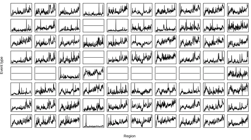
events in each Region with a given event type combination. The series are shown in Figure 1.1.2 where there are 80 possible combinations, however, for some combinations no events occur throughout the entire period and these are shown by horizontal lines in the centre of the grid square.
Region
Ev
[image:22.612.99.500.193.418.2]ent type
Figure 1.1.2: A grid showing all possible combinations of Regions and Event types and the number of events that occur per week for the combination considered.
The primary goal here is to understand the most recent behaviour of the data by analysing all series in the hierarchical time series and fitting a changepoint model to the data.
1.2
Thesis structure
In Chapter 4 we present a novel Bayesian approach to analysing multiple time-series with the aim of detecting abnormal regions. These are regions where the properties of the data change from some normal or baseline behaviour. We allow for the possibility that such changes will only be present in a, potentially small, subset of the time-series. We develop a general model for this problem, and show how it is possible to accurately and efficiently perform Bayesian inference, based upon recursions that enable independent sampling from the posterior distribution. A motivating application for this problem comes from detecting copy number variation (CNVs), using data from multiple individuals. Pooling information across individuals can increase the power of detecting CNVs, but often a specific CNV will only be present in a small subset of the individuals. We evaluate the Bayesian method on both simulated and real CNV data, and give evidence that this approach is more accurate than a recently proposed method for analysing such data.
consideration in this work. This involves pooling information across individual series of the panel to increase the power of detection. We develop a general model for this problem, and show how it is possible to accurately and efficiently perform inference. We present simulations showing that this approach is more accurate than other proposed method for analysing such data. Two real data sets are considered, regarding the number of events that occur over time in a telecommunications network and a data set from the field of Corporate finance where our method gives insights into the different subsets of series that change.
Changepoint detection for univariate
time series
This chapter focuses on changepoint detection in univariate time series. Many of the tech-niques used to analyse multivariate time series described later in this thesis are based upon these univariate methods. Thus understanding them allows us to see their limitations and how they can possibly be extended.
Firstly, in Section 2.2, the changepoint problem is posed as an optimisation problem. Sev-eral different formulations are discussed as well as different solution methods. One of the main concerns is the computational efficiency of the solution methods. We describe several techniques from the literature which are used to reduce the computational complexity of segmenting a time series by an order of magnitude.
In Section 2.3 we then look at modelling changepoints using the Bayesian paradigm, this al-lows more quantification of uncertainty about the locations of changes. However, performing inference for time series of moderate length proves challenging and we find that an acceptably
efficient algorithm comes at the cost of performing approximate inference.
Many of the methods mentioned in this Chapter are implemented in the Changepoint R
package available on CRAN [Killick and Eckley, 2014].
2.1
Notation
Assume we have an ordered sequence of data of lengthnwhich we denotey1:n= (y1, y2, . . . , yn).
Firstly for simplicity consider a single changepoint in the data. Then for some time point
τ ∈ {2, . . . , n−1}, we can split the data into two segments, with the data in the first segment being y1:τ, and that in the second y(τ+1):n. A changepoint model assumes a common model
for data within the same segment but allows different models for data in different segments. Possibly the simplest example is a change in mean model with Normally distributed residuals with some variance σ2. Assume the data in the first segment y
1:τ has a common mean of µ1 and that data in the second segment y(τ+1):n has a different common mean of µ2. The
distribution for this data is as follows Yi ∼ N(µ1, σ2) for i ∈ {1, . . . , τ} and Yj ∼ N(µ2, σ2)
for j ∈ {τ + 1, . . . , n}.
To extend this to the multiple changepoint case, assume there are m changepoints with locations τ1:m = (τ1, τ2, . . . , τm) where τi < τj iff i < j. For notational convenience we define τ0 = 0 and τm+1 = n. These m changepoints segment the data into m+ 1 segments, with
the data in the ith segment being y(τi−1+1):τi.
Y Z
Figure 2.1.1: Three time series having a single change. A mean change on the left, variance change in the middle and change in regression on the right.
2.2
Optimisation methods for changepoint detection
The problem of finding changepoints or, equivalently segmenting a time series into contiguous segments can be formulated as an optimisation problem. This is a popular formulation of the mutiple changepoint detection problem and is the one that the methods in this thesis build on. This formulation gives rise to a relatively simple set of recursions that can be solved exactly to give the location of the changepoints in a time series.
Firstly we discuss two different formulations of the optimisation problem in Sections 2.2.1 and 2.2.2. Efficient methods to perform inference on these two formulations are described in Section 2.2.3.
A penalised cost approach to detecting changepoints involves introducing a cost associated with each putative segment. This cost is often derived by modelling the data within a segment, and then setting the cost to be proportional to minus the maximum likelihood value for fitting that model to a segment of data. If our model for data in a segment is that they are Independently and identically distributed (IID) with some density f(y|θ), where θ
is a segment-specific parameter, then we can define a cost for a segment ys:t as
C(ys:t) =−2 max θ
t
X
i=s
logf(yi|θ).
To make this idea concrete we give an example of a cost function used to model changes in mean. A simple model is that the data in a segment are IID Gaussian with common known variance, σ2, and segment specific mean,θ. In this case we get
C(ys:t) =−2 max
θ −
1 2σ2
t
X
i=s
(yi−θ)2 =
1
σ2
t
X
i=s
yi−
Pt
j=syj t−s+ 1
!2
. (2.2.1)
Once we have defined a segment cost, we then define a cost for a segmentation as the sum of the segment costs for that segmentation.
model to some maximum number of changepoints and the second is to introduce a penalty value each time a changepoint is added. This means that the overall ‘best’ model will provide a good fit using a reasonable amount of changepoints.
The first approach to overcome over-fitting is to consider a constrained optimisation problem where the segmentation is constrained to have a certain number of changepoints (in this case
m)
Qm(y1:n) = min τ1:m
(m+1 X
i=1
C(y(τi−1+1):τi)
)
. (2.2.2)
Usually the number of changes m is unknown so that the number of changes is estimated by minimising the constrained cost plus some penalty which is a function of the number of changes
min
m {Qm(y1:n) +βf(m)}. (2.2.3)
The general form of the penalty function is βf(m). This can be broken down into two parts. Firstly f(m), which is a function of the number of changepoints m. This function is usually chosen to be linear in m. Secondly, β is the term used for model selection (the number of changepoints to be added) which is usually an information theoretic measure. Choices for this term are described in more detail in Section 2.2.4.
constrained problem is known as the penalised optimisation problem. This requires us to take f(m) to be linear in m.
So if f(m) =m and for some β >0, solving (2.2.3) is equivalent to solving
min
m,τ1:m (m+1
X
i=1
C(y(τi−1+1):τi)
+βf(m)
)
, (2.2.4)
which in turn can be written as
min
m,τ1:m
m+1 X
i=1
C(y(τi−1+1):τi) +β
. (2.2.5)
To solve this problem the Optimal Partitioning algorithm described in Section 2.2.2 can be used. Variants of this method are proposed in Section 2.2.3 to decrease the computational cost.
In the following sections we consider the solution of these problems. Both the Segment Neigh-bourhood and Optimal partitioning methods depend on us being able to break the original problem which is difficult to solve into sub problems which are progressively easier to solve via a relatively simple set of recursions. This approach is known as Dynamic programming [Bellman, 1957].
2.2.1
Segment Neighbourhood
The Segment Neighbourhood search algorithm (SN) [Auger and Lawrence, 1989] was devel-oped to solve the constrained optimisation problem described in (2.2.2). In (2.2.2) we defined
the SN recursions we optimise for m changepoints based on the optimal solution for m−1 changepoints. We do this by conditioning on the last changepoint being at s where s < t. Then we can relate Qm(y1:t) to the segmentation ofy1:s withm−1 changepointsQm−1(y1:s)
Qm(y1:t) = min τ1:m
(m+1 X
i=1
C(y(τi−1+1):τi)
)
= min
s∈{τm−1,...,t−1}
Qm−1(y1:s) +C(y(s+1):t)
.
(2.2.6)
Solving this recursion proceeds by going forwards through the data. We need to specify a maximum number of changepoints that we want to consider, say M. We then compute the cost for all possible segmentations, with between 0 and M changepoints.
For each t ∈1, . . . , n we calculate (2.2.6) for all possible change locations, s ∈ m, . . . , t−1. For the full n data points this has computational time of O(n2). This is repeated M times, therefore SN has an overall computational cost ofO(M n2). If, as the observed data increases,
the number of changepoints increases linearly, then M =O(n) and the method will have a computational cost that is cubic in n. This is prohibitive if n is large. One advantage to the SN approach is the ability to use an arbitrary penalty of the form, βf(m) wheref(m) does not have to be linear in m, unlike the Optimal Partitioning method.
2.2.2
Optimal Partitioning
to t is the optimal cost up to s plus the cost of adding a segment from s+ 1 to t (with penalty added as well). Of course we do not know the value of s but we can calculate it via minimising over a set of candidate changepoints for each t.
In order to do this we need to be able to calculate segment costs independently of other segments. This implies that there can be no dependence between the parameters in different segments.
More formally let Tt = {τ : 0 =τ0 < τ1 < . . . < τm < τm+1 =t} be a vector of all possible
segmentations with m changepoints and let F(t) denote the minimisation from (2.2.5) for data y1:t
F(t) = min τ∈Tt
(m+1 X
i=1
C(y(τi−1+1):τi) +β
)
.
Then we can devise a recursion for F(t) as
F(t) = min
s
(
min τ∈Ts
m
X
i=1
C(y(τi−1+1):τi) +β
+C(y(s+1):t) +β
)
,
= min
s
F(s) +C(y(s+1):t) +β .
(2.2.7)
Algorithm 1: Optimal Partitioning algorithm. Input: A data set y1:n= (y1, y2, . . . , yn).
A cost function C(·) dependent on the data. A penalty term β.
Initialize: Let n = the length of the data and set F(0) =−β, cp(0) =N U LL.
for t= 1 to n do
1. Calculate F(t) = min0≤s<t
F(s) +C(y(s+1):t) +β
. 2. Let τ = arg min0≤s<tF(s) +C(y(s+1):t) +β
. 3. Set cp(τ) = (cp(τ), τ)
end
Output: The changepoints recorded incp(n).
In Step 1. of Algorithm 1 for each time step t, we must calculate F(t) by minimising over all the integers between 0 and t−1. Thus for eacht we have to calculatet different expressions and find the minimum. If we have a time series of length n the total number of operations in the full algorithm is of the order of Pn
t=1t ∼ n2. The next section explores how we can
make OP more efficient by removing some integers from consideration.
2.2.3
Pruning
simplest exposition and most efficient algorithm to describe is the OP method. The intuition behind pruning is quite simple if we consider the full OP method.
In the OP algorithm to find F(t) we condition on the most recent changepoint s, prior to
t. This involves searching through all the integers from 0 to t−1 in order to find the best location in which to place the changepoint. Denote the set of candidate changepoints that we must consider at time t as Rt = {0,1, . . . , t−1}. Searching through this entire set of
candidate changepoints Rt at every time step t can be extremely wasteful. For example if we know that the most recent changepoint prior to t is at s then when looking for the most recent changepoint prior to time t+ 1, we should not have to search through the entire list again.
This is where the concept of pruning comes in, we ‘prune’ the setRtremoving those candidate
changepoints that can never be optimal in the future and are left with a smaller subset of
Rt to propagate to the next time step. Intuitively this is clear, however we want the pruned
OP method to remain optimal so we must be careful how we prune Rt.
We now consider two pruning methods that can be used to increase the computational effi-ciency of the OP method whilst ensuring the global minimum of (2.2.5) is still found.
Inequality pruning
Theorem 2.2.1. Killick et al. [2012] Assume there exists a constant K such that for all
t < s < T,
C(y(s+1):t) +C(y(t+1):T) +K ≤ C(y(s+1):T). (2.2.8)
Then, if
F(s) +C(y(s+1):t) +K ≥F(t) (2.2.9)
holds, at a future time T > t, then s can never be the optimal last changepoint prior to T
and so can be removed from all the candidate changepoint sets in the future with no effect on
the exact solution.
Proof. For a proof of this see Section 5 of the supplementary material of Killick et al. [2012].
In condition (2.2.8) if we take cost functions that are based on the log likelihood, such as those described in (2.2.1) we can set K = 0.
Algorithm 2: The PELT algorithm. Input: A data set y1:n= (y1, y2, . . . , yn).
A cost function C(·) dependent on the data. A penalty term β.
A constant K that satisfies Equation (2.2.8).
Initialize: Let n = the length of the data and set F(0) =−β, cp(0) =N U LL,R1 ={0}.
for t= 1 to n do
1. Calculate F(t) = mins∈Rt
F(s) +C(y(s+1):t) +β
. 2. Let τ = arg mins∈Rt
F(s) +C(y(s+1):t) +β
. 3. Set cp(τ) = (cp(τ), τ).
4. Set Rt+1 ={s ∈Rt:F(s) +C(y(s+1):t) +K < F(t)} ∪ {t}
end
Output: The changepoints recorded incp(n).
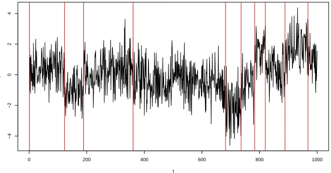
Note how similar this is to the OP algorithm, where the only difference is the addition of the pruning inequality in Step 4. which reduces the size of the candidate changepoint set. In Figure 2.2.1 we show a time series that undergoes a change in mean process which has been segmented with the OP and PELT methods which give identical locations for the changepoints.
Figure 2.2.2 shows the size of the set of candidate changepoints over time i.e. |Rt| for each
time t. For the OP method this line is shown in black and increases linearly with time as |Rt| = t. However, for PELT the corresponding line is in red and with the pruning step
The PELT method is always faster than OP and in certain circumstances when the number of changepoints increases linearly with the length of the data PELT can be shown to beO(n). It performs well in cases where there are a large number of changepoints in the data as lots of pruning can occur throughout time so that the sets Rt cannot grow to be too large.
t
y
0 200 400 600 800 1000
−4
−2
0
2
4
Figure 2.2.1: A time series of length 1000 with the changepoints found using the OP/PELT methods highlighted in red.
0 200 400 600 800 1000
0
200
400
600
800
1000
t
|
Rt
[image:37.612.139.469.196.369.2]|
Functional pruning
Functional pruning, which was first developed by Rigaill [2015] was originally applied to the SN algorithm.
The basic idea behind functional pruning is that conditional on knowing the parameter for the current segment the best location for the most recent changepoint can be calculated easily. Thus only the most recent changepoints that are optimal for some value(s) of the parameter of the current segment need to be considered and the rest can be pruned.
Firstly we define the segmentation cost as a function of the segment parameter which we denote here asθ. A key assumption that underlies functional pruning is that the segmentation costs defined in (2.2.1) can be split into component parts γ(yi, θ) that depend on some
parameter which we minimise over to obtain the overall cost of a segment
C(ys:t) = min θ
t
X
i=s
γ(yi, θ). (2.2.10)
For the change in mean model for Gaussian data the function γ(·) is a quadratic
γ(yi, θ) =
(yi−θ) σ2 .
To develop a set of recursions we follow Maidstone et al. [2016b] and define new cost functions
Costτ
t(θ) as the minimal cost of segmenting the data y1:t with the most recent changepoint
penalty term for a new segment
Costτt(θ) = F(τ) +β+
t
X
i=τ+1
γ(yt, θ). (2.2.11)
Given these cost functions Costτt(θ) we can find F(t) by minimising over both τ and θ by interchanging the order of minimisation
min
τ minθ Cost τ
t(θ) = minτ min θ
"
F(τ) +β+
t
X
i=τ+1
γ(yi, θ)
#
,
= min
τ
"
F(τ) +β+ min
θ t
X
i=τ+1
γ(yi, θ)
#
,
= min
τ
F(τ) +β+C(y(τ+1):t)
,
=F(t).
This relationship is key as it shows that values of the potential last changepoint, τ, can be pruned whilst allowing for a varying θ.
Define the function Cost∗t(θ) as the minimal cost of segmenting data y1:t conditional on the
last segment having parameter θ
Cost∗t(θ) = min
τ Cost τ t(θ).
for Cost∗t(θ) are obtained by splitting the minimisation over τ into τ ≤t−1 andτ =t
Cost∗t(θ) = min
min
τ≤t−1Cost
τ
t(θ), Cost t t(θ)
= minCost∗t−1(θ) +γ(yt, θ), F(t) +β .
To implement these recursions we need to be able to efficiently store and update Cost∗t(θ). This is done by partitioning the space of possibleθvalues, into sets where each set corresponds to a value τ for which Cost∗t(θ) = Costτt(θ). We then need to be able to update these sets, and storeCostτ
t(θ) just for eachτ for which the corresponding set is non-empty. This results
in us storing piece-wise quadratics for the change in mean model.
Functional pruning was combined with the OP algorithm in Maidstone et al. [2016b] result-ing in the Functional Prunresult-ing Optimal Partitionresult-ing (FPOP) algorithm. It was shown that functional pruning always prunes at least as much as inequality based pruning. The FPOP algorithm is especially effective for long data sets which contain few changes for which the PELT algorithm performs poorly.
The FPOP algorithm has seen several modifications, these include the R(obust)-FPOP method [Fearnhead and Rigaill, 2016] which is an approach to changepoint detection that is robust to the presence of outliers. Also the CPOP algorithm [Maidstone et al., 2017a] was developed to fit a continuous piece-wise linear process to a data set.
op-timum for some value of this parameter. Performing this search is easy for a one-dimensional parameter, but computationally intractable for a higher-dimensional parameter. This would occur if we wanted to detect changes in both the mean and variance of a time series at the same time.
2.2.4
Penalty
The penalty function is used to give a parsimonious model that fits the data adequately using a reasonable number of changepoints and so avoids over-fitting.
The general penalty function is βf(m), however, in practice the function that penalises the number of changepoints m, f(m) is linear and increasing in m. For the OP and PELT algorithms we need to take f(m) = m so that we can form the recursion in (2.2.7).
The penalty parameter β has received much more attention in the literature as we rely on this parameter for model selection. In the changepoint problem model selection is basically choosing the “optimal” number of changepoints to put in the data.
The Bayesian Information Criterion (BIC) [Schwarz, 1978] and the Akaike Information Crite-rion (AIC) [Akaike, 1974] are both widely used across statistics for model selection. However, their use in changepoint problems are not theoretically justified, as the likelihood functions involved do not satisfy the required regularity conditions. In Yao [1988] however, weak con-sistency results were established for estimating the number and position of changepoints, in normally distributed data using the BIC penalty.
and variance (µ, σ) then p= 2. The AIC and BIC are then defined as
AIC = 2(p+ 1)
BIC = (p+ 1) logn.
A modified version of the BIC was introduced in Zhang and Siegmund [2007b] which has theoretical justification for one specific model, data consisting of independent normally dis-tributed observations with constant variance and piece-wise constant mean. These informa-tion criteria have also been developed for different and more complex models. For example Ding et al. [2016] derive a consistent BIC like criterion for a piece-wise auto-regressive model. Adaptive procedures for penalty selection were first discussed in Lavielle [August 2005], this leads to the fuller treatment given by the CROPS method [Haynes et al., 2017a]. This paper describes an efficient approach to compare segmentations for different choices of the penalty
β which takes values on some specified continuous range. This method allows us to evaluate the various segmentations and so to identify a suitable choice for the penalty given the specific data set we observe.
2.2.5
Binary Segmentation
The methods we have hitherto described are all exact, meaning they find the optimal solution to the optimisation problem in (2.2.4). Also of interest, and widely applied in practice are approximate methods that do not solve (2.2.4) exactly. These methods can generally be applied more widely to different models and can sometimes be much quicker than their exact counterparts.
A very simple and widely used approximate changepoint method is the Binary segmentation method introduced by Scott and Knott [1974] and Sen and Srivastava [1975]. Binary segmen-tation extends any single changepoint detection method to detect multiple changepoints by repeated application to different subsets of the data. It can be viewed as a greedy heuristic because it makes the locally optimal choice at each stage of the process.
The first step is to apply the chosen single changepoint detection method to the entire data set, if no changepoint is found then we are done. If a changepoint is detected, call thisτ, then the data is split into two segments, y1:τ and y(τ+1):n. We then apply the single changepoint
method to the two segments and repeat iteratively. We stop when no more changepoints are detected.
Assume we are at a step of the algorithm where we consider the segment of data ys:t, firstly
we locate the best location for a single changepoint in this segment of data by minimising
ˆ
τ = arg min
τ∈{s+1,...,t−1}
C(ys:τ) +C(y(τ+1):t)
. (2.2.12)
the fit of the model to warrant its inclusion by testing whether the following inequality holds
C(ys:ˆτ) +C(y(ˆτ+1):t) +β <C(ys:t). (2.2.13)
If this inequality holds then ˆτ is added to the changepoints found and we then split the data into two at time ˆτ so that we have two resulting segments ys:ˆτ and y(ˆτ+1):t. These two new
segments are then analysed using the same procedure, splitting them recursively until the inequality in (2.2.13) does not hold.
Computationally, Binary segmentation is very efficient and is of the order of O(nlogn). The obvious drawback to its use is that it is only approximate in the sense that it does not find the global minimum of (2.2.5), and in certain situations it can break down as estimated change-point locations are conditional on previously identified changechange-points. Practically, however, it often performs very well and the estimated changepoint locations given by this method have been shown to be consistent in a particular sense described in Fryzlewicz [2014b].
There has been some work to develop variants of Binary segmentation in Fryzlewicz [2014b] and Olshen et al. [2004b].
2.3
Bayesian inference for changepoint models
The Bayesian paradigm is also widely used in the changepoint literature. Some examples of these are described in Barry and Hartigan [1993], Green [1995], Fearnhead [2006], Benson and Friel [2016] and Fearnhead and Liu [2007].
The Bayesian approach gives us information regarding the uncertainty in the number of changepoints and their locations from the posterior distribution. This is much more informa-tive than the point estimates given by the optimisation methods mentioned above, however, the disadvantage of Bayesian methods is their larger computational cost.
To perform Bayesian inference we need to specify priors on the parameters of interest, namely the number of changepoints, π(m), locations and segment parameters of the changes condi-tional on the number π(θ(m)|m). The parameter vector θ(m) contains the locations of them
changepoints and the m+ 1 segment specific parameters θi, for i= 1,2, . . . , m+ 1
θ(m) = (τ1, . . . , τm, θ1, . . . , θm+1).
For m changepoints the parameter vector θ(m) has length 2m+ 1. The joint posterior we are interested in can be factorised as
p(m,θ(m)|y)∝π(m)π(θ(m)|m)p(y|θ(m), m). (2.3.1)
differing numbers of changepoints. This is a problem for traditional MCMC samplers as the parameter vector we are aiming to explore and draw samples from θ changes in dimension with each iteration.
One way to perform Bayesian inference on this model is to extend the traditional MCMC methodology and follow the well known Reversible jump Markov chain Monte Carlo (RJM-CMC) method described in Green [1995]. This method allows us to jump between parameter spaces with a different number of dimensions. The traditional MCMC step of proposing a new value for a parameter and deciding whether to accept or reject the move is maintained in the RJMCMC method. However, two more steps are added: a “birth” step, used for the addition of a changepoint to the model and a “death” step, to remove a changepoint. As in standard MCMC the mixing of the chain, autocorrelation of the samples and conver-gence are still an issue here. For general guidelines on designing RJMCMC algorithms see Armstrong et al. [2007]. The problems in diagnosing convergence and the possible substantial errors was highlighted by the analysis of a data set using the RJMCMC method and another approach which we describe below.
An adaptive algorithm was introduced in Benson and Friel [2016] which uses birth and death steps but also learns from the past states of the Markov chain in order to build proposal distributions which can quickly discover where changepoints are likely to be located. It is demonstrated that this algorithm is viable for large datasets and that the MCMC that targets the stationary distribution is ergodic.
extended in Fearnhead [2006]. The advantages of direct simulation methods over MCMC based methods are twofold. Firstly there is no need to concern ourselves with convergence and potentially running the chain for many iterations to prove convergence. Secondly sam-ples from the posterior are independent so quantifying uncertainty is simple. An example of the first problem regarding convergence of the RJMCMC method is clear if we compare the inferences obtained for a Coal-mining disaster data set analysed using RJMCMC in Green [1995] and direct simulation in Fearnhead [2006]. Using the same model resulted in different segmentations because the chain wasn’t run for a sufficient number of iterations.
The disadvantage of direct simulation methods is that they can only be applied to certain changepoint models that satisfy a conditional independence property. In our setting this means that conditional on the changepoint locations parameters of different segments are independent. Many models satisfy this property, for example a change in mean model where the mean parameters of each segment are i.i.d draws from some distribution. However, there are several useful models in practice that do not satisfy this condition. For example if we want to fit piece-wise functions but wish to enforce continuity between functions in neighbouring segments then this introduces dependence between parameters in neighbouring segments. It should be noted that this sort of dependence across segments is a problem for all changepoint detection methods and not only Bayesian methods. Later work in Fearnhead and Liu [2011] showed how the direct simulation method could be adapted to the case where parameters in consecutive segments have a Markov style dependence structure, however their method only calculates an approximation to the posterior.
Fearnhead [2006] and Fearnhead and Liu [2007] are simplest to describe when both the number and position of changepoints are jointly specified via a single prior distribution on the length of a segment. This single prior for the length of a segment implies that the sequence of changepoints forms a discrete renewal process with inter-arrival times that are identically distributed. The simplest inter-arrival distribution commonly used is a geometric distribution which results in the number of changepoints being Binomially distributed. In Section 2.3.1 we show how a series of recursions can be developed following Fearnhead and Liu [2007] to calculate the posterior distribution of interest numerically, and then draw samples from it. We then consider how methods from the particle filtering literature can be used to limit the computational cost of these recursions in Section 2.3.2.
2.3.1
Exact online inference
Following the paper of Fearnhead and Liu [2007] we model the data through a hidden state process, C1:n. This hidden state process will contain information about where the
change-points of the data are located. Our model is defined through specifying the distribution of the hidden state process, p(c1:n), and then the conditional distribution of the data given the
state process, p(y1:n|c1:n).
Our interest lies in inference about this hidden state process given the observations which involves calculating the posterior distribution for the states
p(c1:n|y1:n)∝p(y1:n|c1:n)p(c1:n). (2.3.2)
point prior to time t.
We model Ct as a Markov process, conditional on Ct, either Ct+1 = ct, which corresponds
to no changepoint at time t, or Ct+1 =t, if there is a changepoint at time t. We need that
p(Ct+1 = t|ct) only depends on ct. Thus Ct ∈ {0, . . . , t −1} with Ct = 0 meaning that
the current segment is the first segment. This Markov process is determined by a set of transition probabilities which depend only on the distance between the current time t and the last changepoint.
Due to this process being Markov we can decompose p(c1:n) into factors
p(c1:n) =p(C1 =c1)
n−1 Y
i=1
p(Ci+1 =ci+1|Ci =ci). (2.3.3)
The decomposition in (2.3.3) gives us two aspects of the process to define, namely the tran-sition probabilities p(Ci+1 =ci+1|ci) and the initial distribution, p(C1 =c1).
Firstly consider the transition probabilities. Now either Ct+1 =Ct orCt+1 =t depending on
whether a new segment starts between time t and t+ 1. The probability of a new segment starting is just the conditional probability of a segment being of length t−Ct given that is
at least t−Ct. The probability of a segment continuing is the conditional probability of a
segment having a length greater than t−Ct given that is at least of lengtht−Ct.
1, . . . , t−1 as
p(Ct+1 =j|Ct=i) =
1−G(t−i)
1−G(t−i−1) if j =i
G(t−i)−G(t−i−1)
1−G(t−i−1) if j =t
0 otherwise
This hidden process partitions the time interval into contiguous non-overlapping segments. Using this we want to define a likelihood for the observations conditional on this process
p(y1:n|c1:n), in (2.3.2). To make this model tractable, so we can write down a set of recursions,
we assume a conditional independence between segments:
p(y1:t|Ct=j) = p(y1:j|Ct=j)p(y(j+1):t|Ct=j)
We can then define, for all t < s,
P(t, s) =p(yt:s|Cs=t−1). (2.3.4)
Conditional on the hidden states c1:n the likelihood is
p(y1:n|c1:n) = n
Y
t=1
p(yt|c1:n,y1:t−1)
=
n
Y
t=1
p(yt|ct,y(ct+1):(t−1)).
(2.3.5)
The terms in (2.3.5) can be written as
p(yt|ct,y(ct+1):(t−1)) =
P(ct+ 1, t) P(ct+ 1, t−1)
The main set of recursions is now derived that enable us to calculate the exact posterior numerically. There are two separate cases the first where j < t
p(Ct+1 =j|y1:(t+1))∝p(yt+1|y1:t, Ct+1 =j)p(Ct+1 =j|y1:t)
= P(j+ 1, t+ 1)
P(j+ 1, t) Pr(Ct+1 =j|Ct=j)p(Ct=j|y1:t).
Then the second where j =t
p(Ct+1 =t|y1:(t+1))∝p(yt+1|y1:t, Ct+1 =j)p(Ct+1 =j|y1:t)
=P(t+ 1, t+ 1)
t−1 X
i=0
Pr(Ct+1 =t|Ct=i)p(Ct=i|y1:t).
If we define
wt(+1j) =
P(j+1,t+1)
P(j+1,t) if j < t
P(t+ 1, t+ 1) if j =t
Then we can rewrite the set of recursions above more simply as
p(Ct+1 =j|y1:(t+1))∝
wt(+1j) 1−1−GG(t(−t−i−i)1)p(Ct =j|y1:t) if j < t w(tt+1) Pt−1
i=0
G(t−i)−G(t−i−1)
1−G(t−i−1) p(Ct=i|y1:t)
if j =t
(2.3.7)
Rewriting the recursions in the form shown in (2.3.7) enables us to calculate the posterior distribution ofCt+1 by propagating the posterior for Ct and adding on another support point
for a changepoint at time t.
For many simple models such as a change in mean the weights wt+1 can be calculated
yj+1:t. These summaries can often be calculated and stored before we begin calculating the
recursions and then updated recursively. Indeed for such models the computational cost of calculating any such wt+1 is fixed, and does not increase witht−j.
Simulation
Given that we calculate and store the filtering distributions p(ct|y1:t) for all t = 1, . . . , n,
simulating from the full joint posterior is straightforward. This is done backwards in time by first simulating the last changepoint in the data cn and repeating this until we get to the
beginning of the data.
To simulate one realisation from this joint density:
1. Sett0 =n, and k = 0.
2. Simulate tk+1 from the filtering density p(Ctk|y1:tk), and set k =k+ 1.
3. Iftk >0 return to (2); otherwise output the set of simulated changepoints,tk1, tk2, . . . , t1.
A simple extension of this algorithm allows for efficient simulation of a large sample of realisations of sets of changepoints in a parallel manner. This is described in more detail in Fearnhead [2006].
2.3.2
Approximate filtering
The computational and memory costs of the recursions for exact inference presented in Sec-tion 2.3.1 both increase with time. The filtering distribuSec-tion p(ct|y1:t) has t support points
quadratically in n. The memory costs of storing all of the filtering densities necessary to simulate from the joint posterior of all changepoints also increases quadratically with n. For large data sets, these computational and memory costs become prohibitive.
A similar problem of increasing computational cost occurs in the analysis of some hidden Markov models, though generally computational cost increases exponentially with time [Chen and Liu, 2000]. Particle filters have been successfully applied to these problems [Fearnhead and Clifford, 2003] by using a resampling step to limit the computational cost at each time step. Similar resampling ideas can be applied to the online inference of changepoint models. We follow the methods described by Fearnhead and Liu [2007].
For our problem the particle filtering and resampling methods described here attempt to approximate the discrete distribution p(ct|y1:t) that has t support points with a discrete
distribution with fewer support points or “particles”. This will of course increase the compu-tational efficiency and decrease storage costs. However, due to the nature of these techniques error is introduced in the approximation. The aim is to come up with a method that is a trade off between increased performance while remaining as accurate as possible.
Essentially a threshold value α is chosen that defines the maximum error (as defined by the Kolmogorov Smirnov distance) that is introduced by the resampling procedure at each time step. Then those support points which have a probability less than α are stochastically removed. Note this value α governs the trade-off between a more precise approximation (smaller α) and speed (larger α). The stochastic removal of support points is required so that the process remains unbiased.
in Algorithm 3.
Theoretical guarantees and simulations showing that the SRC algorithm performs well are described in Liu and Chen [1998] and Fearnhead and Liu [2007].
It was found in the analysis of GC content in DNA by Paul Fearnhead [2009] that a value of
α = 10−6introduced negligible error, but greatly increased the speed of the overall algorithm.
The resulting algorithm approximated the filtering densities, by distributions with an average of around 200 support points whereas the true distributions had an average of 80,000 support points, meaning this led to a 400-fold reduction in CPU and memory costs.
Algorithm 3: Stratified rejection control (SRC) Input: An arbitrary cut-off 0< α <1
An ordered set of M particles c(ti) with associated weights w(i) that sum to one, where
i= 1,2, . . . , M.
Initialize: Simulate u a single realisation from Unif(0, α) Set i= 1
while i≤M do if w(i) ≥α then
Keep particle i with weight w(i)
end else
u←u−w(i)
if u≤0then Set w(i)=α u←u+α
end else
Set w(i)= 0
end end
i←i+ 1 end
Output: Remove the particles for whichw(i) = 0 and renormalise the remaining
Changepoint detection for
Multivariate time series
Historically, research on changepoint detection methods has focused on the univariate setting with some of the methods we have looked at in Chapter 2 being developed for this problem. More recently there has been an increased focus on multivariate changepoint detection due to the increase in multivariate series now being collected. There are many sources of this data such as the large array of sensors that record large streaming data sets. This data comes from many diverse fields such as finance where large numbers of asset prices are considered [Cho and Fryzlewicz, 2015] to bioinformatics and signal processing [Vert and Bleakley, 2010]. If we believe that the variables are related somehow and that changepoints occur at the same time in different series, then it makes sense to analyse them together in order to make the best possible use of the information available.
In this setting there are several subtleties that make this problem quite different to its
Figure 3.0.1: A multivariate series with three dimensions where any changes that occur affect all three series at the same time. We call this the full change model.
variate analogue. To show this graphically we have three plots in Figures 3.0.1, 3.0.2 and 3.0.3.
In Figure 3.0.1 we show an example of a three dimensional time series in which both of the changepoints affect all of the dimensions in the series. In future we refer to this problem as the full change model. We can compare this situation to that depicted in Figure 3.0.2 where at each changepoint only a subset of the dimensions are affected, we call this the subset change model.
Another possible subtlety in the multivariate setting is that we can allow for the possibility of different dimensions sharing a common change but the precise location in each dimension is perturbed. We call this the lagged change model and show an example of this in Figure 3.0.3. In the changepoint literature to our knowledge there hasn’t been any work on the lagged change model.
Figure 3.0.2: A multivariate series with three dimensions where the changes that occur only affect a subset of the three series at each changepoint. We call this the subset change model.
Figure 3.0.3: A multivariate series with three dimensions where any changes that occur affect all three series but at slightly different times. We call this the lagged change model.
so we can understand the different types of approaches that have been successful.
3.1
Full change model
[image:58.612.133.478.312.515.2]A simplistic approach to the problem would thus be to try and apply univariate changepoint methods and analyse each time series separately. This method will lose power when detecting changepoints, as it ignores the information that the different time series have changepoints that occur at the same time.
An alternative approach to analysing data of this form is to treat the data as a single time series with multivariate observations. We then model the multivariate data within a segment, and allow for this model to change, in an appropriate way, between segments. This approach is taken by Lavielle and Teyssi`ere [2006], who model data as multivariate Gaussian but with a mean that can change from segment to segment. Lavielle and Teyssi`ere [2006] proposes dynamic programming recursions similar to those described in Chapter 2.
Matteson and James [2014] present a non-parametric approach which is based on a Euclidean style metric known as an energy statistic which takes the role of a cost function. Estima-tion of the changepoint locaEstima-tions is based on hierarchical clustering and both divisive and agglomerative algorithms are developed.
3.2
Subset change model
In some applications, when a changepoint occurs only a subset of the dimensions in a given series are affected. Recently there has been lots of work on certain special cases of the subset change model which are of importance in detecting Copy Number Variants (CNV’s) in Genetics.
important as these variants have been shown to account for much of the variability within a population. More details can be found in Jeng et al. [2013] and the references therein. There are two types of CNV, common CNV which affect all or most of the population and rare CNV which only affect a small subset of the population. Different techniques have been developed to detect the two types of CNV with the methods in Zhang et al. [2010] and Siegmund et al. [2011] designed for the common CNV problem. It was argued in Jeng et al. [2013] that these methods cannot detect rarer CNVs and special methods are required to use the information across the dimensions most efficiently so that it is not drowned out by noise. The Proportion Adaptive Segment Selection (PASS) method developed in Jeng et al. [2013] aims to efficiently detect both common and rare variants without incurring too many false positives.
changepoint to determine the subset of variables each changepoint affects. As estimation is not performed jointly, in that the changepoints and affected variables are not estimated at the same time the methods are approximate. Also when performing the variable specific hypothesis tests problems arise in that certain variables could be falsely claimed to be affected (a Type I error) as well as the converse. For example if many variables were weakly affected by a change but which individually are not significant enough to be flagged by the test (a Type II error). The advantages of both methods, however is that they are relatively computationally efficient and the main idea behind the approaches outlined above is applicable to many different time series models. Indeed Preuss et al. [2015] deviate from the setting of i.i.d. data and aim to detect multiple changes in the autocovariance through the consideration of raw periodograms.
In contrast to the approaches already considered, Pickering [2016] develops a Dynamic pro-gramming method for inference in the full subset change model and outputs changepoint locations as well as the variables that are affected. The two methods (for multivariate data) considered in this thesis are Subset Multivariate Optimal Partitioning (SMOP) and Approximate-SMOP (ASMOP).
The general subset change model is formulated in Pickering [2016] using changepoint vectors. For ap-variate series the changepoint vector at timet,ct= (c
(1)
t , . . . , c
(i)
t , . . . , c
(p)
t ) has length p. The ith element of the vector c(ti) is the location of the most recent change in the ith dimension prior to time t. These vectors encapsulate all the information needed to model the full subset change model.
of a penalised cost function using an exact search. However, this exact search is extremely computationally intensive due to the dependence between segments that exists in the general subset change model. This results in the SMOP method having a computational complexity that is exponential in the length of the data.
An approximate version of this procedure, ASMOP was also presented in this thesis where a substantial reduction in the search space is achieved by identifying “likely” regions in which changepoints are thought to occur and only considering candidates from these areas along with two types of thresholding.
For the univariate and non-parametric case a common and simple approach to detect change-points is to use the CUSUM test [Page, 1954b]. CUSUM statistics are computed over time and track the cumulative distance from the mean for proposed changepoints. These series of CUSUMs are examined to locate changepoints, often where its maximum in the absolute value is attained. With a binary segmentation (BS) algorithm, the CUSUM statistics can consistently detect multiple change-points in a recursive manner (see e.g. Vostrikova [1981], Venkatraman [1993] and Cho and Fryzlewicz [2012]).
This idea can be extended to multivariate data by combining the CUSUMs of each of the dimensions of the series. Care is needed in choosing the method used to combine these. Standard maximum and average methods for doing so often fail in high dimensions when, changepoints only affect a small subset of the series so that the CUSUM statistics are cor-rupted by noise.
high dimensions in order to share information across series. Whenever a thresholding step is introduced in a procedure an additional parameter is usually added. However, the aggregation procedure of Cho [2016] in contrast to Cho and Fryzlewicz [2015], avoids arbitrary choices for the threshold by using a data driven approach which is shown to perform well.
Bayesian detection of abnormal
segments in multiple time series
4.1
Introduction
In this paper we consider the problem of detecting abnormal (or outlier) segments in mul-tivariate time series. We assume that the series has some normal or baseline behaviour but that in certain intervals or segments of time a subset of the dimensions of the series has some kind of altered or abnormal behaviour. By the term abnormal behaviour we mean some change in distribution of the data away from the baseline distribution. For example, this could include a change in mean, variance or auto-correlation structure. In particular our work is concerned with situations where the size of this subset is only a small proportion of the total number of dimensions. We attempt to do this in a fully Bayesian framework. This problem is increasingly common across a range of applications where the detection of abnormal segments (sometimes known as recurrent signal segments) is of interest
larly in high dimensional and/or very noisy data). Some example applications include the analysis of the correlations between sensor data from different vehicles [Spiegel et al., 2011] or for intrusion detection in large interconnected computer networks [Qu et al., 2005]. An-other related application involves detecting common and potentially more subtle objects in a number of images, for example Jin [2004] and the references therein look at this in relation to multiple images taken of astronomical bodies.
We will focus in particular on one specific example of this type of problem, namely that of detecting copy number variants (CNV’s) in DNA sequences. A CNV is a type of structural variation that results in a genome having an abnormal (generally 6= 2) number of copies of a segment of DNA, such as a gene. Understanding these is important as these variants have been shown to account for much of the variability within a population. For a more detailed overview of this topic see Zhang [2010], Jeng et al. [2013] and the references therein.
Data on CNVs for a given cell or individual is often in the form of “log-R ratios” for a range of probes, each associated with different locations along the genome. These are calculated as log base 2 of the ratio of the measured probe intensity to the reference intensity for a given probe. Normal regions of the genome would have log-R ratios with a mean of 0, whereas CNVs would have log-R ratios with a mean that is away from zero.
−3
−1
1
3
−4
−2
0
2
4
−1.0
0.0
1.0
−3
−1
1
3
−2
−1
0
1
2
−4
0
2
4
[image:66.612.125.474.80.432.2]32400 32450 32500
Figure 4.1.1: Log-R ratios from 6 individuals for a small portion of chromosome 16. We indicate the baseline level (mean zero) by a horizontal line in blue and the identified CNV (abnormal region) is highlighted between two vertical black lines with the mean of the affected individuals in red.
for the data in Figure 4.1.1, which shows data from a small portion of chromosome 16, we have identified a single CNV which affects only three individuals. This can seen by the raised means (indicated by the red lines) in these three series for a segment of data. By comparison, the other individuals are unaffected in this segment.
a subset of dimensions has received less attention. Exceptions include methods described in Zhang et al. [2010] and Siegmund et al. [2011]. However Jeng et al. [2013] argue that these methods are only able to detect common variants, that is abnormal segments for which a large proportion of the dimensions have undergone the change. Jeng et al. [2013] propose a method, the PASS algorithm, which is also able to detect rare variants.
suggest that BARD is more accurate than PASS, particularly in terms of having fewer false positives. Furthermore, we see evidence that posterior probabilities are well-calibrated and hence are accurately representing the uncertainty in the inferences. The paper ends with a discussion.
4.2
The Model
We shall now describe the details of our model. Consider a multiple time series of dimension
d and length n, Y1:n = (Y1,Y2, . . . ,Yn) where Yi = (Yi,1, Yi,2, . . . , Yi,d) T
. We model this data through introducing a hidden state process, X1:n. The hidden state process will contain
information about where the abnormal segments of the data are. Our model is defined through specifying the distribution of the hidden state process, p(x1:n), and the conditional
distribution of the data given the state process, p(y1:n|x1:n). These are defined in Sections
4.2.1 and 4.2.2 respectively.
Our interest lies in inference about this hidden state process given the observations. This involves calculating the posterior distribution for the states
p(x1:n|y1:n)∝p(x1:n,y1:n) = p(x1:n)p(y1:n|x1:n). (4.2.1)