The impact of China’s one child policy on intergenerational and gender relations

(1)

Contemporary Social Science

Themed Issue on ‘Family change, intergenerational relations and policy responses’

Guest editors: Fran Bennett, Julia Brannen and Linda Hantrais (corresponding guest

editor)

The impact of China’s one-child policy on intergenerational and gender relations

Yang Hu (Corresponding author),Department of Sociology, Lancaster University Address: Bowland North, Bailrigg, Lancaster University, Lancaster LA1 4YN, UK Email: [email protected]

ORCID: 0000-0003-2027-8491

Yang Hu is a Lecturer in the Department of Sociology at Lancaster University, UK. He is also an early career fellow at the Work Family Researchers Network, USA. His research focuses on the sociology of families and intimate relationships, race/ethnicity and migration, and East Asian societies. He is author of Chinese–British Intermarriage: Disentangling Gender and Ethnicity (Palgrave Macmillan, 2016). He has published in the Journal of Marriage and Family, European Sociological Review, Journal of Sex Research,

Demographic Research, Environment and Planning A, Journal of Family Issues,and British Journal of Sociology of Education.

Xuezhu Shi, Department of Economics, London School of Economics Address: Houghton Street, London, WC2A 2AE, UK

Email: [email protected]

(2)

Xuezhu Shi is a doctoral researcher in the Department of Economics at the London School of Economics, UK. Her research interests are health, gender and family economics in

developing countries, and in China in particular. In her research, she draws on economic theories and uses panel surveys and administrative datasets to examine health, wealth and gender inequalities, and the interrelations between public policies and individual decision-making.

Acknowledgements

The data used in this research are from the China Family Panel Studies (CFPS), funded by the 985 Programme of Peking University and carried out by the Institute of Social Science Survey of Peking University. The authors are solely responsible for the analyses and interpretations presented in this article.

(3)

The impact of China’s one-child policy on intergenerational and gender relations

Abstract

Drawing on data from the China Family Panel Studies, this article assesses the state of gender equality among Chinese children under the one-child policy. We demonstrate the importance of conducting intra-gender and inter-gender comparisons taking into account the perspectives of parents and children and the intergenerational (in)congruence between these two

perspectives. Our results show that parents invest more financial resource and time in educating singleton than non-singleton children, which partially supports the hypothesis of intra-gender equality. The findings for children’s subjective perceptions of their own life circumstances do not consistently support this hypothesis. Since gender differences in intergenerational investment and children’s subjective perceptions varied little by sibship structure, the hypothesis of inter-gender equality is not consistently supported. We found a stronger negative association between the presence of male and elder siblings and

intergenerational investment in girls, and a larger male–female gap in intergenerational investment in urban than in rural areas. We also report a considerable intergenerational incongruence between parents’ and children’s perspectives. Our findings call into question the effectiveness of intervening solely in parental behaviour and intergenerational investment to enhance children’s outcomes. They underline the importance of considering both intra-gender and inter-intra-gender inequalities in moving the intra-gender revolution forward.

Keywords

(4)

Introduction

Introduced in 1979, China’s one-child policy was replaced by the universal two-child policy in 2016 (Wang, Gu, & Cai, 2016). As the world’s most extensive population control policy, the one-child policy has been a major driver of otherwise unlikely demographic shifts in aspects such as family downsizing and the rise of patriarchal demographics featuring a highly skewed sex ratio (Basten & Jiang, 2014). These shifts led to considerable yet unintended changes in intergenerational and gender relations in the Chinese family (Kim & Fong, 2014; Tsui & Rich, 2002). A major change, according to many scholars (Fong, 2004; Lee, 2012), was the rise of gender equality among singleton girls who enjoyed unprecedented

intergenerational support and investment ‘because they do not have to compete with brothers’ for resources (Fong, 2002: 1098), particularly in urban areas (Xu & Yeung, 2013; Zhai & Gao, 2010).

In this article, drawing on data from the China Family Panel Studies (CFPS), we assess the state of gender equality among Chinese children under the one-child policy by examining the ways in which intergenerational investment and children’s subjective perceptions of their own circumstances vary by sibship structure and differ between daughters and sons. In doing so, we make two contributions to existing scholarship. First, claims about rising gender equality under the one-child policy are founded primarily on evidence that, compared to children with siblings, singletons in the one-child generation receive greater financial and time investment from their parents and extended family members (Fong, 2002; Liu, 2016; Tsui & Rich, 2002). We contend that this intra-gender evidence does not suffice to

demonstrate the achievement of gender equality between girls and boys. Underlining the importance of comparison referents, we argue that substantially different evaluation

(5)

comparison between singleton girls and boys and their same-sex counterparts with siblings. Second, following the tradition of social mobility and stratification research, previous and, particularly, quantitative research has focussed on parent-to-child intergenerational transfers (Lee, 2012; Xu & Yeung, 2013; Zhai & Gao, 2010). This approach overlooks children’s subjective views on their own life circumstances, and the presence or absence of gender disparities in such views. Since the gendered pattern of children’s perceptions does not necessarily mirror that of parents’ intergenerational investment, we suggest that scholars should examine the perspectives of both parents and children, and scrutinise the

intergenerational (in)congruence between the two perspectives.

The one-child policy and social change in post-reform China

In 1979, the one-child policy was formally introduced to curb population growth, although the state framed it as a public health policy and claimed that ‘family planning benefits the health of mothers and children’ (see Supplemental Figure S1). Despite the strict enforcement of the policy, particularly at its early stage in the 1980s and early 1990s, exceptions were permitted for certain social groups to have a second child, such as ethnic minorities

(6)

female infanticide to secure male heirs, creating a highly imbalanced sex ratio at birth of an estimated 116 males per 100 females in 2010 (Greenhalgh, 2012).

[Figure 1 about here]

A vast rural–urban gulf underlies the implementation and consequences of the one-child policy (Greenhalgh, 2012; Murphy et al., 2011), as depicted in Figure 1. From its inception, the policy was more rigorously implemented in urban than in rural areas across most Chinese provinces. In 1978–1979, China initiated its market reforms and the open-door policy, which were followed by the state-guided programmes of societal modernisation, privatisation, and urbanisation (Chan, 2015). Due to uneven socioeconomic and cultural development and the rapid rise of urban centres, urban China today remains socioeconomically better off than rural areas, and patrilineal son preference is de-traditionalised to a greater degree in urban than in rural areas (Hu & Scott, 2016). Rural–urban disparities have been exacerbated by the hukou

system, which distinguishes between rural and urban household registration and thereby confers differentiated access to socioeconomic and welfare resources such as medical, education and unemployment subsidies in rural or urban places of registration (Chan, 2015).

The one-child policy and intergenerational gender equality

(7)

children (Hu, 2017). Although patriarchal traditions oblige male more than female children to observe filial obligations (Hu & Scott, 2016), singleton sons and daughters — as the only children in their respective families — may equally be required to ensure their parents’ old-age security (Hu, 2017).

A shift has also occurred in the social, cultural and political context of gender equality in recent decades. Patrilineal son preference has received less support from members of the post-reform generation than from their predecessors (Hu & Scott, 2016). The highly skewed sex ratio may have unintendedly elevated the status of young women as ‘rare’ resources in social arenas such as the marriage market (Greenhalgh, 2012). Under the one-child policy, the presence or absence of siblings and specific sibship structures are imbued with cultural and symbolic meaning. Patrilineal son preference may have encouraged parents to have

multiple children to secure a male heir, despite hefty fines for breaking the law (Murphy et al., 2011). Although ethnic minorities and many rural families were allowed to have a second child, the segmented implementation of the ‘second-child policy’ was inherently selective, with the aim of accommodating the stubborn persistence of patrilineal values in these social groups (Murphy et al., 2011). By contrast, however, parents’ conscious preference to have only one child, and particularly one daughter, may in part reflect their self-selective departure from patrilineal values (Hu, 2017). In recent years, progress toward gender equality may also have been propelled by state and activist campaigns such as the Care for Girl and MeToo movements.

Comparing perspectives: Parents vs children

(8)

life circumstances. The market transition and dissolution of work units unmoored the one-child generation from collectivist and patriarchal traditions (Yan, 2009), fostering a sense of individual personhood (Fong, 2002). Such individuality is often projected through

individualised educational and career aspirations (Fong, 2002; Liu, 2016) and the

self-reflexive approach adopted by singleton children to construct a sense of subjective wellbeing (Kim & Fong, 2014; Wang & Fong, 2009).

However, children’s subjective perception remains largely absent from the assessment of gender equality under the one-child policy. Following the tradition of socioeconomic mobility research, previous studies on China have predominantly focussed on the one-way traffic of parent-to-child care provision and the transfer of economic and human capital (Lee, 2012; Liu, 2016; Xu & Yeung, 2013). Irrespective of parental investment, children construct independent views on their own lived experiences (Fong, 2002; Hu, 2015), and these views may help shape their life aspirations, subjectively perceived sense of gender (in)equality, and subjective wellbeing. In this article, we contend that how children make sense of, and act upon, their own lives is at least as important as the amount of intergenerational investment they receive.

Distinguishing between parents’ and children’s perspectives also enables us to explore potential intergenerational (in)congruence. If familial resources are concentrated on singleton children (compared to children with siblings), and intergenerational investment in singleton girls and boys tends to be equal (Fong, 2002; Kim & Fong, 2014), it is important to

(9)

which children make sense of their lives. Intergenerational (in)congruence also has direct policy relevance, shedding light on the potential effectiveness of intervening solely in adult family members’ behaviour in an attempt to enhance children’s outcomes.

Intra-gender vs inter-gender comparison

It is widely acknowledged that gender equality is defined through relative social comparisons, and such comparisons are conducted in multiple dimensions (Hu & Yucel, 2018). The claim that greater gender equality existed among Chinese children under the one-child policy was based one-sidedly on intra-gender evidence comparing singleton girls and boys to those with siblings (Fong, 2002; Liu, 2016; Xu & Yeung, 2013). Only a small number of studies have considered male–female equality, and conducted inter-gender comparison between singleton daughters and sons (Lee, 2012). It is necessary to distinguish between intra-gender and inter-gender comparisons. Conceptually, the two comparative dimensions represent distinct pathways in the gender revolution. Whilst the former underlines the need to move the gender revolution forward by reducing within-gender disparities, the latter capitalises on the

(10)

Hypotheses

H1 (intra-gender difference): Singleton children enjoy a greater amount of

intergenerational investment (H1A) and more positive subjective perceptions of their life circumstances (H1B) than their counterparts with siblings; and the intra-gender difference between singleton and non-singleton children is greater in urban than in rural areas (H1C).

H2 (inter-gender difference): The gender gap in intergenerational investment (H2A) and children’s subjective perceptions of their life circumstances (H2B) is smaller between singleton girls and boys than that between girls and boys with siblings; and the difference in the female–male gap between singleton and non-singleton children is greater in rural than in urban areas (H2C).

H3 (intergenerational congruence): Differentials in intergenerational investment mediate and thus explain gender and sibship-structure differences in children’s subjective perceptions.

If singleton daughters indeed enjoyed gender equality under the one-child policy, we would expect both Hypothesis 1 and Hypothesis 2, which take account of both parents’ and

children’s perspectives and distinct comparative dimensions, to hold. Due to the persistence of son preference in rural as opposed to urban China (Hu & Scott, 2016), we expect the inter-gender discrepancy between girls and boys to be greater in rural than in urban areas. As the one-child policy was more rigorously implemented and patrilineal ideals are

(11)

differentials in intergenerational investment are primarily responsible for disparities in children’s subjective perceptions, we would expect Hypothesis 3 to hold.

Data and methods

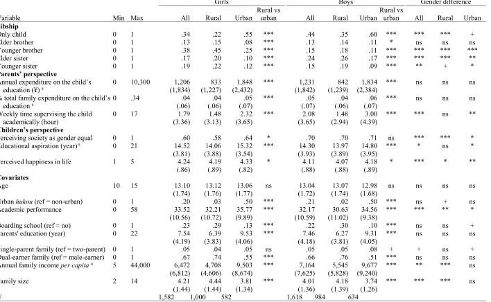
We used data from the 2010 CFPS. In the survey, individual face-to-face interviews were conducted with both child and adult members of the sampled households, thereby capturing the perspectives of both parents and children. Multi-stage probability-proportional-to-size sampling was used to construct a nationally representative sample of 16,000 households from 25 provinces. The response rate at the household level was 81.28%. The self-completion module was only completed by children aged 10–15 in 2010 (N = 3,464). To construct our analytical sample, we first eliminated children outside this age range and 120 children who did not attend school. We then eliminated 144 cases with missing information for key variables (4.2% of the original sample), yielding a final analytical sample of 3,200 school children, of whom 49% were female and 38% were from urban areas. The mean age of the girls was 13.10 and that of the boys was 13.04. The Little’s test was conducted to ensure that our list-wise deletion of missing cases was completely at random. Table 1 displays detailed sample characteristics.

[Table 1 about here]

Dependent variables

(12)

family expenditure represented by educational expenditure on the child; and the total weekly time spent by parents and extended family members on supervising the child’s academic work. No statistically significant gender difference was noted at the 10% level for

intergenerational pecuniary investment. However, a stark rural–urban gap was found in both absolute (t = 15.54, p < .001) and relative (t = 6.34, p < .001) educational expenditure and parents’ non-pecuniary investment of time in their children (t = 9.47, p < .001).

The CFPS also asked the child respondents the following question: ‘Do you think girls are faced with greater pressure than boys in society?’. The survey interviewers were instructed to elaborate on the term ‘pressure’ as the ‘stress and challenge perceived by an individual’. Although the nature and source of ‘stress’ and ‘challenge’ may differ considerably for girls and boys, the measure usefully captures the diffuse sense of gender (in)equality as

subjectively perceived by children. The responses were recorded on a binary ‘yes’ or ‘no’ scale, which we reversed so that the baseline category (‘0’) indicated perceived gender inequality and ‘1’ indicated perceived gender equality. Around two-thirds of the children perceived that, compared to boys, girls are under greater ‘pressure’ in society. A higher proportion of boys (70%) than girls (60%, χ2_{= 36.01,}_{p < .}_{001) perceived society to be}

gender equal, and the rural–urban gulf was noted only among girls (χ2_{= 5.51,}_{p < .}_{05). The}

(13)

responses were recorded on a 5-point scale ranging from ‘very unhappy’ (1) to ‘very happy’ (5). On balance, urban children reported enjoying greater happiness in their lives than their rural counterparts (t = 3.87, p < .001).

Sibship structure

The key independent variables were a series of dummy variables capturing children’s sibship structure, i.e. whether the children had one or more elder and younger brothers, elder and younger sisters, respectively. As it was rare for more than one person to appear in each sibship role, we coded as ‘yes’ (1) cases in which a child had one or more siblings in a given sibship position. We experimented with disaggregating each sibling position by more specific age groups, such as pre-school and school-age. However, this distinction was not found to make a statistically significant difference to the outcome variables, and did not contribute to increasing the overall model fit. It was therefore excluded from our final analysis.

The results confirm that the one-child policy has only been loosely implemented, particularly in rural areas, as 34% of the girls and 44% of the boys were the only children in their

respective families. While 57% of the urban children were the only children in their

respective families, only 28% of the rural children were the only child (χ2 _{= 3.87,}_p_{< .001).}

The results also delineate a nuanced demographic reality under the policy: Whereas the girls (38%) were much more likely than the boys (15%) to have younger brothers (χ2_{= 202.40,}_p < .001), the boys (24%) were more likely than the girls (17%) to have elder sisters (χ2₌

(14)

Covariates

We controlled for children’s age and its quadratic form to account for non-linearity. As well as distinguishing between rural and urban (38%) location of residence, we controlled for rural vs urban (20.5%) hukou (household registration) status (Chan, 2015). Children’s academic performance may influence both their self-perception and the educational investment they receive from parents. We measured the children’s academic performance by adding up their scores in standardised maths and literacy tests conducted as part of the CFPS. We included a dummy variable for boarding school (zhudu) attendance (22.9%), as this may influence the time children could spend with their parents and siblings as well as children’s own sense of independence. We also controlled for parents’ years of schooling (M = 7.50, SD = 4.19) and single-parenthood (5.4%). As parents’ gender roles may influence gendered intergenerational relations (Hu, 2015), we distinguished dual-earner families (66.6%) from male-earner

families. At the family level, we also controlled for annual family income per capita and the number of routine residents in the household (M = 4.12, SD = 1.40) (see online supplemental material for the covariates tested in our preliminary analysis but excluded from this article).

Analytical strategy

We used hierarchical regression models with random intercepts at the family level to account for the clustering of multiple children within the same family and any unobserved

(15)

interaction terms between rural vs urban residence and the sibship dummies were then added to the models to explore rural–urban differences. The second set of models were fitted using the full sample to enable inter-gender comparison between boys and girls across sibship structures. Similarly, the rural–urban interaction terms were added to the models. Third, we included the intergenerational investment measures in the models predicting children’s subjective perceptions to test whether differences in the former mediated the relationships between sibship, gender and rural/urban residence, respectively, and children’s subjective perceptions. To aid the interpretation of the results and conserve space, we graphed the marginal effects for the key variables (see supplemental online material for full results). The variance inflation factor (VIF values < 5) test was conducted to ensure that no

multicollinearity existed between the predictors. Although parents may self-select to have more than one child, our additional tests correcting for this selection yielded results that were consistent with those reported in this article. This may be because the self-selection is closely related to, and thus captured by, observed traits such as rural vs urban hukou and residence (for example differentiated endorsement of patrilineal values) and family socioeconomic status such as capability to pay fines.

Findings

In this section, we first present the intra-gender comparative findings, separately for girls and boys. We then present the inter-gender comparative findings. Lastly, we report the results for the intergenerational (in)congruence between the perspectives of children and parents.

Intra-gender comparison: Girls

(16)

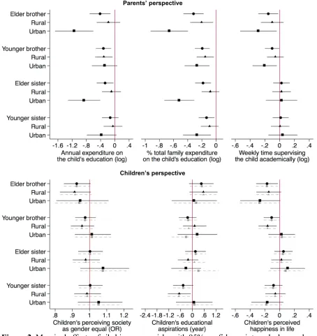
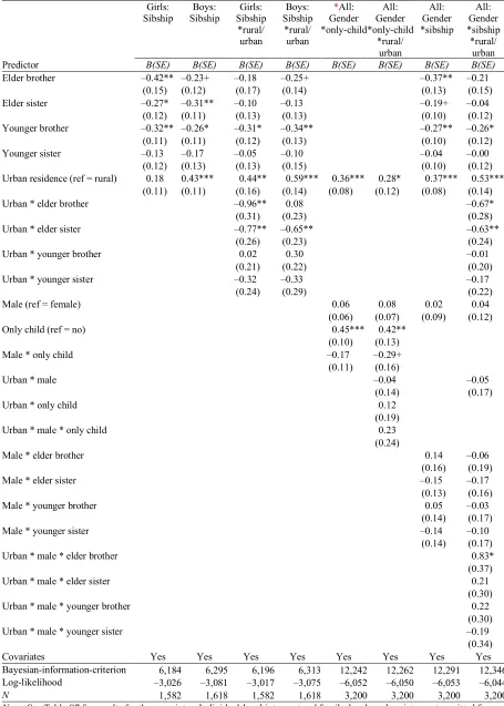
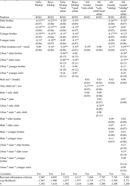
Figure 2 depicts the marginal effects of sibship on intergenerational investment in girls and on their subjective perceptions. The results support Hypothesis 1A: Compared to singleton girls, those with siblings received less financial investment in their education. Specifically, financial investment in girls’ education was negatively associated with the presence of

younger brothers, elder brothers and elder sisters, respectively, but not that of younger sisters. These negative associations were found to be similar in both the absolute amount of

investment and the relative proportion of the family’s total expenditure represented by such investment. The proportion of family expenditure spent on girls’ education was negatively associated with the presence of younger sisters. These findings are consistent with China’s traditional patriarchal hierarchy, which gives precedence to male and elder siblings: the distribution of resources trickles down the gender-cum-age lineage (Hu & Scott, 2016). Moreover, a low level of correlation was found between financial and non-pecuniary

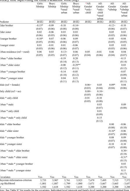
investment in girls (Pearson’s r = .09, p < .10), and sibship seemed to have varying effects on intergenerational time and financial investment in girls’ education. Parents spent less time supervising their daughters academically in the presence of male but not female siblings.

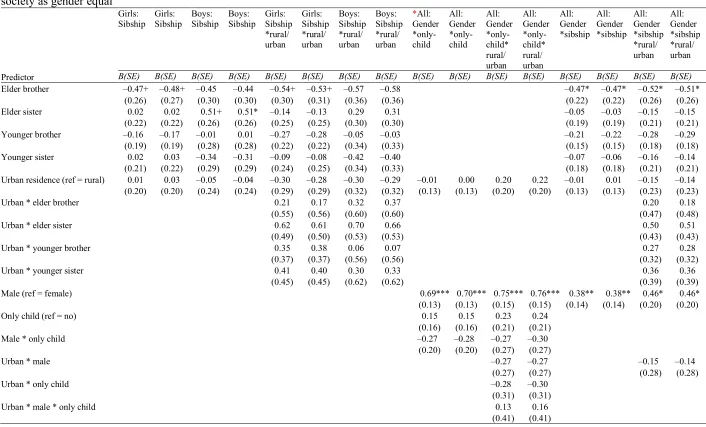
The results do not consistently support Hypothesis 1B, as the girls’ subjective perceptions and aspirations varied little by sibship structure. Only a few exceptions were noted.

(17)

particularly younger brothers (B = –0.16, p < .01) reported feeling less happy with life than their singleton counterparts.

Supporting Hypothesis 1C, the negative associations between the presence of siblings and intergenerational investment of both financial resources and time in girls were stronger in urban than in rural areas. In part, this may be because of the higher cost associated with raising a child and tighter time constraints faced by parents in urban as opposed to rural areas.

Intra-gender comparison: Boys

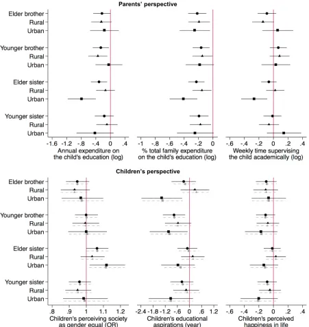
Figure 3 depicts the results for boys’ intra-gender comparisons. Hypothesis 1A is supported by the results: The presence of siblings consistently predicted a smaller proportion of

intergenerational investment in boys’ education relative to total family expenditure. In terms of boys’ subjective perceptions, the results do not consistently support Hypothesis 1B. The presence of elder sisters positively predicts the perception of urban boys that girls and boys are faced with similar levels of ‘pressure’ in society (OR = 1.12, p< .05). In urban areas, elder sisters may serve as role models for their younger brothers, sending positive signals regarding gender equality (Lu & Trieman, 2008). Urban boys with elder brothers (B = –1.37,

(18)

No consistent empirical support was found for Hypothesis 1C. Compared to singleton boys, boys with elder brothers in rural areas (B = –0.25, p < .10), younger brothers in rural areas (B = –0.34, p < .01) and elder sisters in urban areas (B = –0.79, p < .001) received less financial investment in their education. No consistent rural–urban differences were observed in the associations between sibship structure and intergenerational investment in boys and in boys’ subjective perceptions.

Inter-gender comparison: Girls and boys

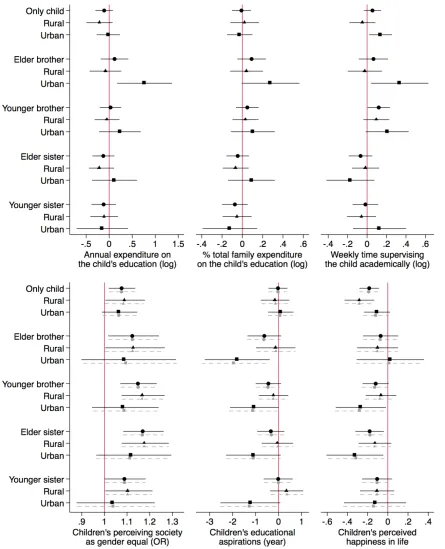
Figure 4 depicts the marginal differences between girls and boys in intergenerational

investment and in children’s subjective perceptions across sibship structures. The findings do not support Hypothesis 2A, which predicts that singleton boys and girls enjoy greater inter-gender equality in intergenerational investment than their counterparts with siblings (see Liu, 2016; Tsui & Rich, 2002). We found little gender difference (at the 5% level) in

intergenerational investment, irrespective of sibship structure. The only exception was that urban parents invested more in the education of boys with elder brothers than girls with elder brothers, in terms of both financial resources (Bmale-female = 0.77, p < .05) and time (Bmale-female

= 0.34, p < .05).

(19)

counterparts, rural girls and boys were more likely to differ in their views on the presence (or absence) of differentiated levels of societal ‘pressure’ on girls and boys.

No statistically significant gender difference was found in educational aspiration among singleton children. In families with siblings, however, girls had higher educational aspirations than boys, particularly in urban areas. This finding may have two concurrent explanations. First, boys with siblings may be less likely to perceive themselves as their families’ ‘only hope’, reducing their aspirations relative to those of singleton boys (Fong, 2004). Second, girls with siblings may attach particular value to education as a means of changing their gendered fate (Lee, 2012), resulting in high aspirations.

On balance, the girls reported having enjoyed greater happiness in life than the boys. The gender gap was particularly prominent among singleton children in rural areas (Bmale-female = – 0.28, p < .01). This may be because, compared to rural girls with siblings, singleton girls in rural areas are less likely to live in families that closely endorse patrilineal ideals. In urban areas, the gender gap in children’s perceived happiness in life was prominent among children with younger brothers (Bmale-female = –0.27, p < .05) and elder sisters (Bmale-female = –0.33, p

< .05), respectively. These results may be related to the divergent ways in which urban girls and boys are influenced by the presence of younger brothers and elder sisters. Whereas urban boys’ perceived happiness in life was negatively associated with the presence of younger brothers and elder sisters (see Figure 3), urban girls with younger brothers and particularly elder sisters enjoyed greater happiness in life than their singleton counterparts (see Figure 2). These results may partly reflect the de-traditionalisation of patrilineal values in urban China (Hu & Scott, 2016). As a result, it is unlikely that the presence of younger brothers

(20)

as it may do in rural areas. By contrast, the presence of elder sisters may act as a positive role model that helps to enhance girls’, but not boys’, subjective wellbeing in urban areas (Lu & Trieman, 2008).

Comparative perspectives and intergenerational incongruence

In Figures 2, 3 and 4, the grey dashed lines represent the marginal effects of the models, including intergenerational financial and time investment, in predicting children’s subjective perceptions. Our findings did not support Hypothesis 3 that differentials in intergenerational investment mediate and therefore explain disparities in children’s subjective perceptions. The inclusion of intergenerational investment measures made almost no difference to the marginal effects of sibship, gender and rural–urban residence on children’s subjective perceptions. This intergenerational incongruence may in part be due to the (re)production of cross-generational gender inequalities through channels other than the intercross-generational pecuniary and non-pecuniary investment investigated in this research, such as the gendered

performance of domesticity (Hu, 2015), marital orientation and mobility (Hu, 2016), and gendered work and occupational orientations (Bian, 2002).

Conclusions

(21)

First, our findings show that substantially different evaluative outcomes may arise from intra-gender and inter-intra-gender comparison. Singleton children received more financial investment in their education than their non-singleton counterparts; and parents spent less time

supervising girls’ academic work in the presence of male siblings. These findings may appear to support the argument that, under the one-child policy, Chinese families were able to

concentrate their resources on their singleton children (Wang & Fong, 2009). Nevertheless, the results from inter-gender comparisons revealed little discrepancy in intergenerational investment of money and time in the education of boys and girls, irrespective of sibship structure. Arguably, the resource concentration on singleton children — girls and boys alike — may simply be an artefact of the financial strain faced by families with multiple children (as opposed to one-child families), which may affect the available resources parents can invest in a given child rather than the ways in which resources are distributed. The discrepant findings of the intra-gender and inter-gender comparisons challenge the assumption that the intra-gender advantages enjoyed by singleton daughters over their non-singleton counterparts (Fong, 2002; Liu, 2016) can readily add up to female–male gender equality. Therefore, it is pertinent to consider both intra-gender and inter-gender disparities in moving the gender revolution forward (Hu & Yucel, 2018).

(22)

findings also suggest that differentials in parental behaviour across sibship conditions cannot be assumed to explain how children make sense of their own lives. The results therefore problematise the assumption undergirding mainstream policy interventions in China that gender equality among children can be achieved solely by changing the ways in which parents behave and by equalising intergenerational investment (Zhai & Gao, 2010).

Third, our findings problematise the assumption that greater gender equality may exist among urban as opposed to rural children under the one-child policy (Fong, 2002; Fong, 2004). The results for rural–urban disparity differed considerably between parents’ and children’s perspectives. Consistent with the observation that urbanites adhere less closely to patriarchal values than rural Chinese (Hu & Scott, 2016), we found that rural boys and girls differed more than their urban counterparts in their perceived sense of societal ‘pressure’ on them. In contrast, however, the negative association between the presence of male and elder siblings and intergenerational investment in girls’ education was stronger in urban than in rural areas. This observation may be attributed to an endogenous selection effect: given the strict

implementation of the one-child policy and hefty extra-child fines in urban China (Murphy et al., 2012), urbanites who chose to break the policy may have a particularly strong preference for sons, although the overall level of adherence to patrilineality remains stronger in rural than in urban areas (Hu & Scott, 2016).

The limitations of our study indicate several promising directions for further research. First, intergenerational relations and the progress toward gender equality are dynamic, and are closely embedded in their socio-historical contexts. Yet our analysis provided only a static snapshot of the dynamic processes. Ideally, future efforts should be made to collect

(23)

temporal dynamics of intergenerational and gender relations under the one-child policy and the new universal two-child policy. Second, our analysis focused specifically on the

intergenerational relations between parents and adolescent children. However, given the rapid pace of population ageing in China, members of the one-child generation may soon take on the responsibility of providing socioeconomic support and care for their elderly parents and grandparents. As the life course dynamics of the singleton children unfold, future scholars could usefully explore how the one-child family structure may influence the potentially gendered provision of old-age care in a multigenerational framework.

References

Basten, S., & Jiang, Q. (2014). China’s family planning policies: Recent reforms and future prospects. Studies in Family Planning, 45(4), 493–509. https://doi.org/10.1111/j.1728-4465.2014.00003.

Bian, Y. (2002). Chinese social stratification and social mobility. Annual Review of Sociology,

28(1), 91–116. doi: 10.1146/annurev.soc.28.110601.140823

Chan, K.W. (2015). Five decades of the Chinese hukou system. In R.R. Iredale & F. Guo (Eds.), Handbook of Chinese migration: Identity and wellbeing (pp. 23-47). Cheltenham: Edward Elgar. doi: 10.4337/9781783476640

Fong, V.L. (2002). China’s one-child policy and the empowerment of urban daughters.

American Anthropologist, 104(4), 1098–1109. doi: 10.1525/aa.2002.104.4.1098

Fong, V.L. (2004). Only hope: Coming of age under China’s one-child policy. CA: Stanford University Press.

(24)

mainland China. Journal of Marriage and Family, 79(3), 739–757. https://doi.org/10.1111/jomf.12391

Hu, Y. (2015). Gender and children’s housework time in China: Examining behavior modeling in context. Journal of Marriage and Family, 77(5), 1126–1143. doi: 10.1111/jomf.12225

Hu, Y. (2016). Marriage of matching doors: Marital sorting on parental background in China.

Demographic Research, 35, 557–580. doi: 10.4054/DemRes.2016.35.20

Hu, Y., & Scott, J. (2016). Family and gender values in China: Generational, geographic, and gender differences. Journal of Family Issues, 37(9), 1267–1293. doi:

10.1177/0192513X14528710

Hu, Y., & Yucel, D. (2018). What fairness? Gendered division of housework and family life satisfaction across 30 countries. European Sociological Review, 34(1), 92–105.

https://doi.org/10.1093/esr/jcx085

Kim, S.W., & Fong, V.L. (2014). A longitudinal study of son and daughter preference among Chinese only-children adolescence to adulthood. The China Journal, 71(1), 1–24. doi:10.1086/674551

Lee, M.H. (2012). The one-child policy and gender equality in education in China: Evidence from household data. Journal of Family and Economic Issues, 33(1), 41–52. doi: 10.1007/s10834-011-9277-9

Liu, Y. (2016). Women rising as half of the sky? An empirical study on women from the one-child generation and their higher education participation in contemporary China. Higher Education, 1–16. doi: 10.1007/s10734-016-0102-0

Lu, Y., & Treiman, D.J. (2008). The effect of sibship size on educational attainment in China: Period variations. American Sociological Review, 73(5), 813–834. doi:

(25)

Murphy, R., Tao, R., & Lu, X. (2011). Son preference in rural China: Patrilineal families and socioeconomic change. Population and Development Review, 37(4), 665–690. doi: 10.1111/j.1728-4457.2011.00452.x

Tsui, M., & Rich, L. (2002). The only child and educational opportunity for girls in urban China. Gender & Society, 16(1), 74–92. doi: 10.1177/0891243202016001005

Wang, F., Gu, B., & Cai, Y. (2016). The end of China’s one-child policy. Studies in Family Planning, 47(1), 83–86. doi: 10.1111/j.1728-4465.2016.00052.x

Wang, Y., & Fong, V.L. (2009). Little emperors and the 4:2:1 generation: China’s singletons.

Journal of the American Academy of Child & Adolescent Psychiatry, 48(12), 1137–1139. doi: 10.1097/CHI.0b013e3181bc72f8

Xu, Q., & Yeung, W.J.J. (2013). Hoping for a phoenix: Shanghai fathers and their daughters.

Journal of Family Issues, 34(2), 184–209. doi: 10.1097/CHI.0b013e3181bc72f8 Yan, Y. (2009). The individualization of Chinese Society. London: Bloomsbury.

(26)

Variable Min Max All Rural Urban Rural vs urban All Rural Urban Rural vs urban All Rural Urban

Sibship

Only child 0 1 .34 .22 .55 *** .44 .35 .60 *** *** *** +

Elder brother 0 1 .13 .15 .08 *** .13 .14 .11 * ns ns ns

Younger brother 0 1 .38 .45 .25 *** .15 .18 .11 *** *** *** ***

Elder sister 0 1 .17 .20 .10 *** .24 .26 .17 *** *** *** **

Younger sister 0 1 .19 .22 .12 *** .15 .19 .09 *** ** + *

Parents’ perspective

Annual expenditure on the child’s

education (¥) a 0 10,300 _(1,834)1,206 _(1,227)833 _(2,432)1,848 *** _(1,842)1,231 _{(1,239) (2,384)}842 1,834 *** ns ns ns

% total family expenditure on the child’s

education a 0 .34 _(.06).04 _(.06).04 _(.07).05 *** _(.07).05 _(.06).04 _(.07).06 *** ns ns ns

Weekly time supervising the child

academically (hour) 0 17 (3.36) 1.79 (3.13) 1.48 (3.65) 2.32 *** (3.65) 2.08 (2.94) 1.48 (4.39) 3.00 *** *** ns **

Children’s perspective

Perceiving society as gender equal 0 1 .60 .58 .64 * .70 .70 .71 ns *** *** *

Educational aspiration (year) a ₀ ₂₁ _14.52 _14.06 _15.32 _*** _14.30 _13.97 _{14.80 ***} _* _ns _*

(3.81) (3.88) (3.54) (3.93) (3.89) (3.95)

Perceived happiness in life 1 5 4.24 4.19 4.33 * 4.11 4.07 4.18 * *** * **

(.86) (.89) (.82) (.88) (.88) (.89)

Covariates

Age 10 15 13.10 13.12 13.06 ns 13.04 13.07 12.98 ns ns ns ns

(1.74) (1.76) (1.77) (1.72) (1.74) (1.68)

Urban hukou (ref = non-urban) 0 1 .20 .03 .50 *** .21 .02 .50 *** ns + ns

Academic performance 0 58 33.52 32.21 35.77 *** 32.17 30.63 34.56 *** *** ** *

(10.56) (10.72) (9.89) (10.59) (11.02) (9.38)

Boarding school (ref = no) 0 1 .23 .29 .13 *** .22 .30 .10 *** ns ns +

Parents' education (year) 0 22 7.54 6.39 9.53 *** 7.46 6.27 9.31 *** ns ns ns

(4.19) (3.83) (4.06) (4.18) (3.81) (4.05)

Single-parent family (ref = two-parent) 0 1 .05 .04 .05 ns .05 .05 .08 + + ns +

Dual-earner family (ref = male-earner) 0 1 .67 .74 .55 *** .66 .76 .51 *** ns ns ns

Annual family income per capitaa ₅ _44,000 _6,472 _4,708 _9,503 _*** _7,164 _5,545 _{9,677 ***} _** _*** _ns

(6,812) (4,606) (8,674) (7,625) (5,828) (9,240)

Family size 2 14 4.21 4.44 3.81 *** 4.01 4.18 3.74 *** *** *** ns

(1.44) (1.44) (1.34) (1.36) (1.39) (1.26)

N 1,582 1,000 582 1,618 984 634

Note: a_{Top 1% replaced to be equal to the 99}th_{percentile to minimise the influence of outlier cases. Standard deviations in parenthesis. Mean score for continuous}

[image:26.842.66.774.68.504.2]

(27)

[image:27.595.146.450.72.261.2]

Figure 1. Gender ratio at birth in China 1982–2010, by rural–urban context

(28)

[image:28.595.70.524.62.543.2]

Figure 2. Marginal effects ofsibship among girls, with 95% confidence intervals, by rural– urban residence (reference = singleton girls, N =1,582).

Note: OR = Odds Ratio.

Logistic regression for perceived gender equality. All covariates held constant.

(29)

[image:29.595.73.524.60.536.2]

Figure 3. Marginal effects ofsibship among boys, with 95% confidence intervals, by rural– urban residence (reference = singleton boys, N = 1,618).

(30)

[image:30.595.75.520.59.608.2]

Figure 4. Marginal male-female differences, with 95% confidence intervals, by sibship status and rural/urban residence (reference = female, N = 3,200).

(31)

for

The impact of China’s one-child policy on intergenerational and gender relations

In this document, we present further contextual information about the one-child policy and full results for the two-level random-intercept regression models. In Figure S1, we present an official poster promoting the one-child policy as a public health campaign, instead of a population control policy.

(32)

[image:32.595.183.414.54.395.2]

Figure S1. ‘Family planning benefits the health of mothers and children’. Poster created and produced by the Family Planning Office of Kunming, circa 1978.

Source: National Library of Medicine, National Institute of Health, USA.

(33)

annual expenditure on the child’s education (log)

Girls:

Sibship Sibship Boys: Sibship Girls: *rural/ urban Boys: Sibship *rural/ urban *All: Gender *only-child All: Gender *only-child *rural/ urban All: Gender *sibship All: Gender *sibship *rural/ urban

Predictor B(SE) B(SE) B(SE) B(SE) B(SE) B(SE) B(SE) B(SE)

Elder brother –0.42** –0.23+ –0.18 –0.25+ –0.37** –0.21 (0.15) (0.12) (0.17) (0.14) (0.13) (0.15)

Elder sister –0.27* –0.31** –0.10 –0.13 –0.19+ –0.04

(0.12) (0.11) (0.13) (0.13) (0.10) (0.12) Younger brother –0.32** –0.26* –0.31* –0.34** –0.27** –0.26*

(0.11) (0.11) (0.12) (0.13) (0.10) (0.12)

Younger sister –0.13 –0.17 –0.05 –0.10 –0.04 –0.00

(0.12) (0.13) (0.13) (0.15) (0.10) (0.12) Urban residence (ref = rural) 0.18 0.43*** 0.44** 0.59*** 0.36*** 0.28* 0.37*** 0.53***

(0.11) (0.11) (0.16) (0.14) (0.08) (0.12) (0.08) (0.14)

Urban * elder brother –0.96** 0.08 –0.67*

(0.31) (0.23) (0.28)

Urban * elder sister –0.77** –0.65** –0.63**

(0.26) (0.23) (0.24)

Urban * younger brother 0.02 0.30 –0.01

(0.21) (0.22) (0.20)

Urban * younger sister –0.32 –0.33 –0.17

(0.24) (0.29) (0.22)

Male (ref = female) 0.06 0.08 0.02 0.04

(0.06) (0.07) (0.09) (0.12)

Only child (ref = no) 0.45*** 0.42**

(0.10) (0.13)

Male * only child –0.17 –0.29+

(0.11) (0.16)

Urban * male –0.04 –0.05

(0.14) (0.17)

Urban * only child 0.12

(0.19)

Urban * male * only child 0.23

(0.24)

Male * elder brother 0.14 –0.06

(0.16) (0.19)

Male * elder sister –0.15 –0.17

(0.13) (0.16)

Male * younger brother 0.05 –0.03

(0.14) (0.17)

Male * younger sister –0.14 –0.10

(0.14) (0.17)

Urban * male * elder brother 0.83*

(0.37)

Urban * male * elder sister 0.21

(0.30)

Urban * male * younger brother 0.22

(0.30)

Urban * male * younger sister –0.19

(0.34)

Covariates Yes Yes Yes Yes Yes Yes Yes Yes

Bayesian-information-criterion 6,184 6,295 6,196 6,313 12,242 12,262 12,291 12,346 Log-likelihood –3,026 –3,081 –3,017 –3,075 –6,052 –6,050 –6,053 –6,044

N 1,582 1,618 1,582 1,618 3,200 3,200 3,200 3,200

Note: See Table S7 for results for the covariates. Individual-level intercept and family-level random intercepts omitted from the table.

[image:33.595.68.523.85.722.2]

(34)

the percentage of total family expenditure spent on the child’s education (log)

Girls:

Sibship Sibship Boys: Sibship Girls: *rural/ urban Boys: Sibship *rural/ urban *All: Gender *only-child All: Gender *only-child*rural/ urban All: Gender *sibship All: Gender *sibship* rural/ urban

Elder brother –0.32*** –0.22*** –0.20* –0.19* –0.26*** –0.18* (0.07) (0.06) (0.08) (0.08) (0.06) (0.07) Elder sister –0.18*** –0.23*** –0.08 –0.15* –0.14** –0.05

(0.06) (0.06) (0.06) (0.07) (0.05) (0.05) Younger brother –0.19*** –0.16** –0.15* –0.14* –0.17*** –0.12*

(0.05) (0.06) (0.06) (0.07) (0.05) (0.06) Younger sister –0.13* –0.19** –0.09 –0.17* –0.09+ –0.06

(0.06) (0.07) (0.06) (0.07) (0.05) (0.06) Urban residence (ref = rural) 0.06 0.10+ 0.24** 0.19* 0.10* –0.00 0.11* 0.24***

(0.06) (0.06) (0.08) (0.07) (0.04) (0.06) (0.04) (0.07)

Urban * elder brother –0.46** –0.06 –0.28*

(0.15) (0.13) (0.14)

Urban * elder sister –0.44*** –0.26* –0.35**

(0.12) (0.11) (0.11)

Urban * younger brother –0.12 –0.04 –0.13

(0.10) (0.12) (0.10)

Urban * younger sister –0.18 –0.07 –0.10

(0.11) (0.14) (0.10)

Male (ref = female) 0.03 0.03 0.02 0.06

(0.03) (0.03) (0.04) (0.06)

Only child (ref = no) 0.27*** 0.17**

(0.05) (0.06)

Male * only child –0.04 –0.00

(0.05) (0.08)

Urban * male 0.02 –0.07

(0.07) (0.08)

Urban * only child 0.26**

(0.09)

Urban * male * only child –0.06

(0.11)

Male * elder brother 0.09 0.02

(0.08) (0.09)

Male * elder sister –0.07 –0.11

(0.06) (0.07)

Male * younger brother 0.05 0.01

(0.06) (0.08)

(0.07) (0.08)

Urban * male * elder brother 0.27

(0.18)

Urban * male * elder sister 0.19

(0.14) Urban * male * younger

brother

0.09

(0.14)

Urban * male * younger sister –0.09

(0.16)

N 1,582 1,618 1,582 1,618 3,200 3,200 3,200 3,200

[image:34.595.73.525.84.729.2]

(35)

weekly time supervising the child’s academic work (log)

Girls:

Sibship Sibship Boys: Sibship Girls: *rural/ urban Boys: Sibship *rural/ urban *All: Gender *only-child All: Gender *only-child *rural/ urban All: Gender *sibship All: Gender *sibship *rural/ urban

Elder brother –0.15* –0.09 –0.10 –0.14+ –0.12+ –0.10

(0.07) (0.06) (0.08) (0.08) (0.06) (0.07)

Elder sister 0.02 –0.06 0.03 0.03 0.05 0.03

(0.06) (0.05) (0.06) (0.06) (0.05) (0.06)

Younger brother –0.10* 0.07 –0.06 0.09 –0.05 –0.04

(0.05) (0.06) (0.06) (0.07) (0.05) (0.05)

Younger sister 0.01 –0.01 0.01 –0.06 0.05 0.03

(0.05) (0.06) (0.06) (0.07) (0.05) (0.06) Urban residence (ref = rural) 0.06 0.03 0.13+ 0.06 0.05 –0.01 0.06 0.04

(0.05) (0.05) (0.07) (0.07) (0.04) (0.06) (0.04) (0.07)

Urban * elder brother –0.19 0.20 –0.13

(0.14) (0.13) (0.14)

Urban * elder sister –0.00 –0.29** 0.03

(0.12) (0.11) (0.12)

Urban * younger brother –0.14 –0.05 –0.07

(0.10) (0.12) (0.09)

Urban * younger sister 0.04 0.21 0.04

(0.11) (0.13) (0.11)

Male (ref = female) 0.06+ 0.05 0.09* 0.04

(0.03) (0.04) (0.04) (0.06)

Only child (ref = no) 0.08+ 0.10+

(0.05) (0.06)

Male * only child –0.01 –0.10

(0.05) (0.08)

Urban * male 0.03 0.09

(0.07) (0.08)

Urban * only child 0.01

(0.09)

Urban * male * only child 0.15

(0.12)

Male * elder brother 0.00 –0.06

(0.08) (0.10)

Male * elder sister –0.16* –0.06

(0.07) (0.08)

Male * younger brother 0.08 0.09

(0.07) (0.08)

Urban * male * elder brother 0.30+

(0.18)

Urban * male * elder sister –0.31*

(0.15)

Urban * male * younger brother 0.03

(0.15)

Urban * male * younger sister 0.11

(0.17)

N 1,582 1,618 1,582 1,618 3,200 3,200 3,200 3,200

[image:35.595.75.522.79.737.2]

(36)

[image:36.842.71.777.92.519.2]

Table S4. Results for the key variables from two-level random-intercept logistic regression models predicting the odds of children’s perceiving society as gender equal

Girls:

Sibship Girls: Sibship Boys: Sibship Boys: Sibship Girls: Sibship *rural/ urban Girls: Sibship *rural/ urban Boys: Sibship *rural/ urban Boys: Sibship *rural/ urban *All: Gender *only-child All: Gender *only-child All: Gender *only-child* rural/ urban All: Gender *only-child* rural/ urban All: Gender *sibship All: Gender *sibship All: Gender *sibship *rural/ urban All: Gender *sibship *rural/ urban

Predictor B(SE) B(SE) B(SE) B(SE) B(SE) B(SE) B(SE) B(SE) B(SE) B(SE) B(SE) B(SE) B(SE) B(SE) B(SE) B(SE)

Elder brother –0.47+ –0.48+ –0.45 –0.44 –0.54+ –0.53+ –0.57 –0.58 –0.47* –0.47* –0.52* –0.51* (0.26) (0.27) (0.30) (0.30) (0.30) (0.31) (0.36) (0.36) (0.22) (0.22) (0.26) (0.26) Elder sister 0.02 0.02 0.51+ 0.51* –0.14 –0.13 0.29 0.31 –0.05 –0.03 –0.15 –0.15

(0.22) (0.22) (0.26) (0.26) (0.25) (0.25) (0.30) (0.30) (0.19) (0.19) (0.21) (0.21) Younger brother –0.16 –0.17 –0.01 0.01 –0.27 –0.28 –0.05 –0.03 –0.21 –0.22 –0.28 –0.29

(0.19) (0.19) (0.28) (0.28) (0.22) (0.22) (0.34) (0.33) (0.15) (0.15) (0.18) (0.18) Younger sister 0.02 0.03 –0.34 –0.31 –0.09 –0.08 –0.42 –0.40 –0.07 –0.06 –0.16 –0.14

(0.21) (0.22) (0.29) (0.29) (0.24) (0.25) (0.34) (0.33) (0.18) (0.18) (0.21) (0.21) Urban residence (ref = rural) 0.01 0.03 –0.05 –0.04 –0.30 –0.28 –0.30 –0.29 –0.01 0.00 0.20 0.22 –0.01 0.01 –0.15 –0.14

(0.20) (0.20) (0.24) (0.24) (0.29) (0.29) (0.32) (0.32) (0.13) (0.13) (0.20) (0.20) (0.13) (0.13) (0.23) (0.23)

Urban * elder brother 0.21 0.17 0.32 0.37 0.20 0.18

(0.55) (0.56) (0.60) (0.60) (0.47) (0.48)

Urban * elder sister 0.62 0.61 0.70 0.66 0.50 0.51

(0.49) (0.50) (0.53) (0.53) (0.43) (0.43)

Urban * younger brother 0.35 0.38 0.06 0.07 0.27 0.28

(0.37) (0.37) (0.56) (0.56) (0.32) (0.32)

Urban * younger sister 0.41 0.40 0.30 0.33 0.36 0.36

(0.45) (0.45) (0.62) (0.62) (0.39) (0.39)

Male (ref = female) 0.69*** 0.70*** 0.75*** 0.76*** 0.38** 0.38** 0.46* 0.46* (0.13) (0.13) (0.15) (0.15) (0.14) (0.14) (0.20) (0.20)

Only child (ref = no) 0.15 0.15 0.23 0.24

(0.16) (0.16) (0.21) (0.21)

Male * only child –0.27 –0.28 –0.27 –0.30

(0.20) (0.20) (0.27) (0.27)

Urban * male –0.27 –0.27 –0.15 –0.14

(0.27) (0.27) (0.28) (0.28)

Urban * only child –0.28 –0.30

(0.31) (0.31)

Urban * male * only child 0.13 0.16

(37)

Male * elder brother 0.08 0.08 0.02 0.01 (0.29) (0.29) (0.35) (0.35)

Male * elder sister 0.46+ 0.45+ 0.40 0.40

(0.25) (0.25) (0.29) (0.29)

Male * younger brother 0.32 0.32 0.35 0.35

(0.24) (0.24) (0.29) (0.29)

Male * younger sister –0.09 –0.09 –0.09 –0.09

(0.25) (0.25) (0.30) (0.30)

Urban * male * elder brother 0.06 0.11

(0.64) (0.65)

Urban * male * elder sister 0.00 –0.03

(0.57) (0.57)

Urban * male * younger brother –0.25 –0.23

(0.52) (0.52)

Urban * male * younger sister –0.12 –0.12

(0.59) (0.59) Covariate Yes Yes Yes Yes Yes Yes Yes Yes Yes Yes Yes Yes Yes Yes Yes Yes Parental investment No Yes No Yes No Yes No Yes No Yes No Yes No Yes No Yes Bayesian-information-criterion 2,209 2,228 2,057 2,076 2,236 2,254 2,084 2,104 4,173 4,192 4,195 4,214 4,206 4,226 4,273 4,293 Log-likelihood –1,042 –1,040 –966 –964 –1,040 –1,039 –965 –963 –2,022 –2,019 –2,021 –2,018 –2,014 –2,012 –2,011 –2,009

N 1,582 1,582 1,618 1,618 1,582 1,582 1,618 1,618 3,200 3,200 3,200 3,200 3,200 3,200 3,200 3,200

(38)

[image:38.842.73.765.85.516.2]

Table S5. Results for the key variables from two-level random-intercept models predicting children’s educational aspirations Girls: Sibship Girls: Sibship Boys: Sibship Boys: Sibship Girls: Sibship *rural/ urban Girls: Sibship *rural/ urban Boys: Sibship *rural/ urban Boys: Sibship *rural/ urban *All: Gender *only-child All: Gender *only-child All: Gender *only-child *rural/ urban All: Gender *only-child *rural/ urban All: Gender *sibship All: Gender *sibship All: Gender *sibship *rural/ urban All: Gender *sibship *rural/ urban

Elder brother 0.45 0.48 –0.29 –0.21 0.57 0.56 0.27 0.34 0.28 0.35 0.41 0.44 (0.31) (0.31) (0.30) (0.30) (0.36) (0.36) (0.36) (0.36) (0.30) (0.30) (0.35) (0.35) Elder sister 0.15 0.16 –0.11 –0.04 0.12 0.11 0.16 0.19 0.07 0.09 0.11 0.11

(0.26) (0.26) (0.25) (0.25) (0.30) (0.30) (0.29) (0.29) (0.26) (0.26) (0.29) (0.29) Younger brother –0.24 –0.21 –0.76** –0.75** –0.22 –0.19 –0.56+ –0.57+ –0.37+ –0.33 –0.30 –0.27

(0.23) (0.23) (0.28) (0.28) (0.26) (0.26) (0.33) (0.33) (0.21) (0.21) (0.26) (0.25) Younger sister –0.47+ –0.47+ –0.38 –0.33 –0.67* –0.68* –0.16 –0.11 –0.53* –0.52* –0.65* –0.65* (0.26) (0.26) (0.29) (0.29) (0.29) (0.29) (0.32) (0.32) (0.25) (0.25) (0.29) (0.29) Urban residence (ref = rural) –0.01 –0.03 –0.37 –0.39 –0.06 –0.11 0.17 0.13 –0.14 –0.17 0.16 0.15 –0.14 –0.18 0.06 –0.00

(0.24) (0.24) (0.24) (0.24) (0.34) (0.34) (0.32) (0.32) (0.17) (0.18) (0.27) (0.27) (0.17) (0.17) (0.31) (0.31)

Urban * elder brother –0.47 –0.35 –1.64** –1.67** –0.32 –0.21

(0.67) (0.67) (0.60) (0.60) (0.66) (0.66)

Urban * elder sister 0.14 0.20 –0.73 –0.61 –0.04 0.03

(0.58) (0.58) (0.49) (0.49) (0.58) (0.58)

Urban * younger brother –0.10 –0.12 –0.47 –0.42 –0.11 –0.09

(0.44) (0.44) (0.56) (0.56) (0.44) (0.44)

Urban * younger sister 0.76 0.79 –0.76 –0.81 0.57 0.59

(0.53) (0.53) (0.62) (0.62) (0.53) (0.53)

Male (ref = female) –0.24 –0.26 0.04 0.03 –0.17 –0.19 –0.21 –0.23

(0.16) (0.16) (0.19) (0.19) (0.19) (0.19) (0.27) (0.27)

Only child (ref = no) 0.09 0.02 0.09 0.04

(0.22) (0.22) (0.29) (0.29)

Male * only child 0.22 0.24 –0.19 –0.16

(0.26) (0.26) (0.36) (0.36)

Urban * male –1.05** –1.06** 0.13 0.12

(0.36) (0.36) (0.38) (0.38)

(0.42) (0.42)

Urban * male * only child 1.31* 1.28*

(0.55) (0.55)

(39)

(0.40) (0.40) (0.48) (0.48)

Male * elder sister –0.10 –0.06 0.10 0.13

(0.33) (0.33) (0.39) (0.39)

Male * younger brother –0.25 –0.26 –0.12 –0.13

(0.32) (0.32) (0.39) (0.39)

Male * younger sister 0.29 0.31 0.58 0.60

(0.34) (0.34) (0.40) (0.40)

Urban * male * elder brother –1.33 –1.48+

(0.88) (0.88)

Urban * male * elder sister –0.68 –0.65

(0.74) (0.74) Urban * male * younger

brother

–0.46 –0.48

(0.70) (0.70)

Urban * male * younger sister –1.29 –1.32+

(0.80) (0.80) Covariates Yes Yes Yes Yes Yes Yes Yes Yes Yes Yes Yes Yes Yes Yes Yes Yes Parental investment No Yes No Yes No Yes No Yes No Yes No Yes No Yes No Yes Bayesian-information-criterion –4,244 –4,240 –4,393 –4,388 –4,243 –4,239 –4,388 –4,383 –8,639 –8,634 –8,633 –8,628 –8,631 –8,626 –8,624 –8,619 Log-likelihood 8,621 8,635 8,919 8,931 8,648 8,662 8,938 8,950 17,414 17,429 17,427 17,442 17,448 17,462 17,506 17,520

N 1,582 1,582 1,618 1,618 1,582 1,582 1,618 1,618 3,200 3,200 3,200 3,200 3,200 3,200 3,200 3,200

(40)

[image:40.842.66.769.79.518.2]

Table S6. Results for the key variables from two-level random-intercept models predicting children’s perceived happiness in life Girls:

Sibship Sibship Girls: Sibship Boys: Sibship Boys: Sibship Girls: *rural/ urban Girls: Sibship *rural/ urban Boys: Sibship *rural/ urban Boys: Sibship *rural/ urban *All: Gender *only-child All: Gender *only-child All: Gender *only-child *rural/ urban All: Gender *only-child *rural/ urban All: Gender *sibship All: Gender *sibship All: Gender *sibship *rural/ urban All: Gender *sibship *rural/ urban

Elder brother –0.17* –0.17* –0.10 –0.09 –0.15+ –0.15+ –0.11 –0.10 –0.17* –0.17* –0.16+ –0.15+ (0.07) (0.07) (0.07) (0.07) (0.08) (0.08) (0.08) (0.08) (0.07) (0.07) (0.08) (0.08) Elder sister 0.05 0.04 –0.02 –0.01 0.02 0.02 0.03 0.03 0.03 0.03 0.00 0.00

(0.06) (0.06) (0.06) (0.06) (0.07) (0.07) (0.07) (0.07) (0.06) (0.06) (0.07) (0.07) Younger brother –0.11* –0.11* –0.11 –0.11+ –0.16** –0.16** –0.08 –0.08 –0.13* –0.12* –0.19** –0.19**

(0.05) (0.05) (0.07) (0.07) (0.06) (0.06) (0.08) (0.08) (0.05) (0.05) (0.06) (0.06) Younger sister –0.08 –0.09 –0.09 –0.08 –0.06 –0.06 –0.05 –0.04 –0.11+ –0.11* –0.10 –0.10

(0.06) (0.06) (0.07) (0.07) (0.07) (0.07) (0.08) (0.08) (0.06) (0.06) (0.07) (0.07) Urban residence (ref = rural) 0.02 0.02 0.02 0.02 –0.02 –0.02 0.09 0.09 0.02 0.02 0.04 0.05 0.02 0.03 –0.04 –0.03

(0.06) (0.06) (0.06) (0.06) (0.08) (0.08) (0.07) (0.07) (0.04) (0.04) (0.06) (0.06) (0.04) (0.04) (0.07) (0.07)

Urban * elder brother –0.12 –0.12 0.04 0.04 –0.10 –0.11

(0.16) (0.16) (0.14) (0.14) (0.16) (0.16)

Urban * elder sister 0.08 0.06 –0.16 –0.15 0.09 0.08

(0.13) (0.13) (0.12) (0.12) (0.14) (0.14)

Urban * younger brother 0.19+ 0.20+ –0.09 –0.08 0.19+ 0.19+

(0.10) (0.10) (0.13) (0.13) (0.10) (0.10)

Urban * younger sister –0.11 –0.12 –0.15 –0.17 –0.09 –0.10

(0.12) (0.12) (0.14) (0.14) (0.13) (0.13)

Male (ref = female) –0.09* –0.09* –0.06 –0.06 –0.17*** –0.17*** –0.24*** –0.24*** (0.04) (0.04) (0.04) (0.04) (0.04) (0.04) (0.06) (0.06)

Only child (ref = no) 0.12* 0.11* 0.17* 0.16*

(0.05) (0.05) (0.07) (0.07)

Male * only child –0.10 –0.10 –0.22* –0.22*

(0.06) (0.06) (0.09) (0.09)

Urban * male –0.09 –0.09 0.14 0.13

(0.09) (0.09) (0.09) (0.09)

(0.10) (0.10)

Urban * male * only child 0.26* 0.26*

(0.13) (0.13)

(41)

(0.09) (0.09) (0.11) (0.11)

Male * elder sister –0.04 –0.03 0.05 0.05

(0.08) (0.08) (0.09) (0.09)

Male * younger brother 0.04 0.03 0.14 0.13

(0.07) (0.07) (0.09) (0.09)

Male * younger sister 0.05 0.05 0.07 0.08

(0.08) (0.08) (0.10) (0.10)

Urban * male * elder brother 0.13 0.12

(0.21) (0.21)

Urban * male * elder sister –0.27 –0.24

(0.18) (0.18) Urban * male * younger

brother

–0.29+ –0.29+

(0.16) (0.16)

Urban * male * younger sister –0.04 –0.05

(0.19) (0.19) Covariates Yes Yes Yes Yes Yes Yes Yes Yes Yes Yes Yes Yes Yes Yes Yes Yes Parental investment No Yes No Yes No Yes No Yes No Yes No Yes No Yes No Yes Bayesian-information-criterion 4,034 4,048 4,230 4,244 4,058 4,071 4,256 4,271 8,148 8,157 8,167 8,176 8,186 8,195 8,250 8,259 Log-likelihood –1,951 –1,947 –2,048 –2,045 –1,948 –1,944 –2,047 –2,043 –4,005 –3,998 –4,003 –3,995 –4,000 –3,993 –3,996 –3,988

N 1,582 1,582 1,618 1,618 1,582 1,582 1,618 1,618 3,200 3,200 3,200 3,200 3,200 3,200 3,200 3,200

(42)

[image:42.595.77.524.100.396.2]

Table S7. Results for the covariates from two-level random-intercept models (N = 3,200 for all models)

Annual expenditure on the child’s

education (log)

% of total family expenditure on the child’s

education Weekly time supervising the child academically (log) Children’s perceiving society as gender equal Children’s educational aspirations Children’s perceived happiness in life

Covariate B(SE) B(SE) B(SE) B(SE) B(SE) B(SE)

Age –0.69** –0.28* –0.52*** –0.47 –0.48 –0.19

(0.26) (0.12) (0.13) (0.47) (0.62) (0.15)

Age2 _0.03** _0.01* _0.02** _0.01 _0.00 _0.00

(0.01) (0.00) (0.00) (0.02) (0.02) (0.01)

Urban hukou (ref = rural) 0.48*** 0.26*** 0.20*** 0.40* 0.81*** –0.03

(0.10) (0.05) (0.05) (0.16) (0.22) (0.05)

Academic performance 0.02*** 0.01*** –0.01*** 0.00 0.09*** 0.01***

(0.00) (0.00) (0.00) (0.01) (0.01) (0.00)

Boarding school (ref = no) 0.71*** 0.46*** –0.12*** 0.04 0.25 0.03

(0.07) (0.03) (0.03) (0.12) (0.17) (0.04)

Parents’ schooling years 0.03*** 0.00 0.04*** –0.01 0.10*** 0.01*

(0.01) (0.00) (0.00) (0.01) (0.02) (0.00)

Single-parent family (ref = no) –0.23+ 0.02 –0.14* 0.02 –0.10 –0.21**

(0.14) (0.07) (0.06) (0.22) (0.30) (0.07)

Dual-earner family (ref = male-earner) –0.08 –0.03 0.06+ 0.11 0.19 0.05

(0.07) (0.03) (0.03) (0.11) (0.15) (0.03)

Family income per capita (log) 0.32*** –0.03+ 0.04* –0.02 0.28*** 0.05**

(0.04) (0.02) (0.02) (0.06) (0.08) (0.02)

Family size –0.01 –0.05*** 0.04** –0.04 –0.03 –0.01

(0.03) (0.01) (0.01) (0.04) (0.06) (0.01)

Note: Because the results for the covariates predicting each dependent variable changed little across the models with different specifications of the key predictors, we report the results for the covariates based on the full samples (models marked by a red asterisk ‘*’). The results continue from the first models for the full sample in Tables S1–S6. Individual-level intercept and family-level random intercepts omitted from the table.