ISSN Online: 2152-7393 ISSN Print: 2152-7385
DOI: 10.4236/am.2018.98067 Aug. 30, 2018 985 Applied Mathematics
Modeling and Numerical Solution of a Cancer
Therapy Optimal Control Problem
Melina-Lorén Kienle Garrido
1, Tim Breitenbach
1, Kurt Chudej
2, Alfio Borzì
1 1Institut für Mathematik, Universität Würzburg, Würzburg, Germany2Lehrstuhl für Wissenschaftliches Rechnen, Fakultät für Mathematik, Physik und Informatik,
Universität Bayreuth, Bayreuth, Germany
Abstract
A mathematical optimal-control tumor therapy framework consisting of ra-dio- and anti-angiogenesis control strategies that are included in a tumor growth model is investigated. The governing system, resulting from the com-bination of two well established models, represents the differential constraint of a non-smooth optimal control problem that aims at reducing the volume of the tumor while keeping the radio- and anti-angiogenesis chemical dosage to a minimum. Existence of optimal solutions is proved and necessary condi-tions are formulated in terms of the Pontryagin maximum principle. Based on this principle, a so-called sequential quadratic Hamiltonian (SQH) me-thod is discussed and benchmarked with an “interior point optimizer—a mathematical programming language” (IPOPT-AMPL) algorithm. Results of numerical experiments are presented that successfully validate the SQH solu-tion scheme. Further, it is shown how to choose the optimisasolu-tion weights in order to obtain treatment functions that successfully reduce the tumor vo-lume to zero.
Keywords
Cancer, Radiotherapy, Anti-Angiogenesis, Sparse Controls, Optimal Control, Pontryagin’s Maximum Principle, SQH Method
1. Introduction
Cancer has a growing impact on our society, because it is among the main causes of illness and death worldwide. On account of this, there exist many treatment options as surgery, chemotherapy, radiation therapy, hormonal therapy, immu-notherapy and anti-angiogenic treatment. For all these therapies, it is important
How to cite this paper: Kienle Garrido, M.-L., Breitenbach, T., Chudej, K. and Borzì, A. (2018) Modeling and Numerical Solution of a Cancer Therapy Optimal Control Problem. Applied Mathematics, 9, 985-1004.
https://doi.org/10.4236/am.2018.98067
Received: July 23, 2018 Accepted: August 27, 2018 Published: August 30, 2018
Copyright © 2018 by authors and Scientific Research Publishing Inc. This work is licensed under the Creative Commons Attribution International License (CC BY 4.0).
DOI: 10.4236/am.2018.98067 986 Applied Mathematics to balance the benefits of each treatment with its negative side effects. Therefore a natural mathematical approach to cancer therapy is to consider a mathematical model of the time evolution of tumor that includes the action of the therapy as a control mechanism with the purpose to minimize the tumor volume, while keeping at a minimum the negative side effects on the healthy cells. In order to find an optimal therapy, we formulate an optimal control problem that requires to minimize the tumor volume in a given time horizon and to maximize the health-related quality of life of the patient.
Concerning previous works on optimal control in drug therapy, we refer to, e.g., [1][2][3]. However, while these references discuss models for immunothe-rapy, the combination of radiation therapy and anti-angiogenic treatment as in
[4] and in our work is not considered. Another new aspect of our cancer therapy model is the combination of two tumor growth systems, one proposed by Hahn-feld et al.[5] and the other one by Ergun et al.[6]. We discuss our model in Sec-tion 2, where we illustrate the inclusion of control mechanisms and provide val-ues of the model’s parameters that result from real data.
The typical optimization objective used in cancer therapy models that are considered in the literature is to minimize the tumor volume at the terminal time; see [3] and [4]. In this paper, we investigate a more general cost functional that corresponds to minimizing the tumor volume along the entire time horizon and including L1- and L2-costs of the treatment modelled by the control
func-tions. In Section 2.3, we discuss this new cost functional and formulate our op-timal control problem. In Section 3, we provide a detailed analysis of our tumor development and treatment model and discuss equilibrium points of this dy-namical system and the positivity of solutions. In Section 4, we prove existence of optimal solutions to our optimal control problem and their characterization by the optimality conditions in the framework of the Pontryagin maximum principle (PMP). In Section 5, we illustrate the sequential quadratic Hamiltonian (SQH) method. Also in this section, we consider the operating mode of the “in-terior point optimizer—a mathematical programming language” (IPOPT-AMPL) solver that we use as a benchmark for our optimization method, before we focus on our SQH scheme. In Section 6, we present results of numerical experiments that successfully validate the effectiveness of our numerical optimization proce-dure that computes the same results as the IPOPT-AMPL scheme, while requir-ing considerably less time. Further, we use our SQH solution scheme to show that it is possible to set the optimisation weights in such a way to obtain treat-ment functions that successfully reduce the tumor volume to zero. A section of conclusion completes this work.
2. Mathematical Modeling of Cancer Development and
Treatment
DOI: 10.4236/am.2018.98067 987 Applied Mathematics models consider the dynamics between the tumor volume p and the carrying capacity q. One of the most commonly used models for tumor growth is based on the Gompertzian growth law as follows
( )
(
ln)
, 0.p p a = −ξ p a> >ξ
While the proliferation rate a of the cells is constant, the death rate ξln
( )
p increases with a growing tumor volume p. The value q, where the proliferation rate equals the death rate, is called the carrying capacity given byexp a .
q= ξ Using this normalized carrying capacity, we obtain
( )
( )
ln ln exp ln ln .
a a p
p p p p p p
q
ξ ξ ξ
ξ ξ
= − = − = −
(1)
For p q< the tumor grows (p>0) until p q= . For p q> the tumor shrinks (p<0) again until p q= is reached.
Next, we consider a time-varying carrying capacity q. The basic idea is a com-bination of stimulatory (S) and inhibitory (I) effects as follows
(
,) (
, .)
q S p q= −I p q
A modelling issue is the choice of S and I, and for this reason we consider the model proposed by Hahnfeldt et al.[5] as follows
2 3 ,
q bp dp q= − (2) with the birth rate b>0 and the death rate d>0. This is a well-recognized
mathematical model for time-varying carrying capacity. However, it couples the tumor volume variable to the carrying capacity.
On the other hand, a model of time-varying carrying capacity that does not involve the tumor volume explicitly is due to Ergun et al. [6]. This model is computationally convenient since p does not appear in the equation. We have
2 4
3 3.
q bq= −dq (3) Based on validation with real data [5] [6], both models appear promising in the quest of an accurate description of tumor growth. For this reason, we con-sider a combination of the two models (2) and (3) as follows
(
)
2 4 2
3 3 1 3 ,
q=κbq −dq + −κ bp dp q−
where κ∈
[ ]
0,1 . Together with the equation for the tumor growth (1), weob-tain the following differential system that models the evolution of the tumor vo-lume and of the carrying capacity of the vasculature. We have
(
)
2 4 2
3 3 3
ln p , 1 .
p p q bq dq bp dp q
q
ξ κ κ
= − = − + − −
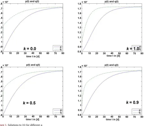
DOI: 10.4236/am.2018.98067 988 Applied Mathematics In Figure 1, we show the evolution of this system for initial values with
( )
0( )
0p <q and for different
κ
. We see that the dynamics obtained with0
κ= , that is with (2), dominates the evolution of our model given by (4). The
model (4) exhibits a steep increase at the initial time for the variable q for
0≤ ≤κ 0.5 and, choosing
κ
close to one a slower increase of q can be ob-served. From this result, it appears that κ =0.5 andκ
=1 are representativeof two different dynamical behaviour and we shall consider these choices in the numerical experiments.
In the next two sections, we introduce two control mechanisms in (4) that represent the treatment of cancer by anti-angiogenesis and radiotherapy, respec-tively [3].
2.1. Anti-Angiogenesis
[image:4.595.68.536.314.722.2]The angiogenesis is a process where a growing tumor develops its own blood vessels, which provide the tumor with oxygen and nutrients. The anti-angiogenesis
DOI: 10.4236/am.2018.98067 989 Applied Mathematics therapy is an indirect treatment since it does not fight the tumor cells directly but influences the tumor’s micro-environment, in particular the vasculature. The lack of oxygen and nutrients will force the tumor to shrink.
To model this treatment, we introduce a control u that takes its values in
[
0,umax]
and represents the dose of the anti-angiogenic medicine. With thean-ti-angiogenic elimination parameter γ >0, we can augment the equation for q
in (4) as follows
(
)
2 4 2
3 3 1 3 .
q=κbq −dq + −κ bp dp q− −γqu
Hence, our model for an anti-angiogenetic mono-therapy is given by
(
)
2 4 2
3 3 3
ln p , 1 .
p p q bq dq bp dp q qu
q
ξ κ κ γ
= − = − + − − −
(5)
The anti-angiogenic treatment influences the carrying capacity of the vascu-larity q, but as q appears in the equation for p, it also influences the tumor vo-lume p.
2.2. Radiotherapy
Radiotherapy is a treatment that uses ionizing radiation to kill cancer cells. For this purpose and to minimize damage on healthy tissues the tumor should be well localized.
To model this treatment, we introduce the control w, which represents the dose of radiation and takes its values in
[
0,wmax]
. Following a model from Wein et al.[7], the damage that is done to the tumor by radiation is modelled as fol-lows( )
(
( )
( ))
( )
0 e d ,
t t s
p t α β w s −ρ − s w t
− +
∫
with the radiosensitive parameters α β, >0 depending on the treated tissue
and the tissue repair rate ρ>0. To simplify the expression above, we introduce the function
( )
( )
( ) 0: t e t sd .
r t = w s −ρ − s
∫
This is the solution to a linear ODE given by
( )
, 0 0.
r= −ρr w r+ =
Hence, the term that quantifies the damage done to the tumor can be written as follows
(
α βr pw)
.− +
Now, we have to take into account that the radiation has also a damaging ef-fect on the healthy tissues. Specifically, the damage on the carrying capacity of the vascularity q is given by
(
η δr qw)
.DOI: 10.4236/am.2018.98067 990 Applied Mathematics Notice that the radiosensitive parameters η δ, >0 have different values,
be-cause malignant and healthy tissues have different characteristics.
Summarizing, our controlled model of cancer’s development and treatment is given by
(
)
(
)
(
)
2 4 2
3 3 3
ln ,
1 ,
.
p
p p r pw
q
q bq dq bp dp q qu r qw
r r w
ξ α β
κ κ γ η δ
ρ
= − − +
= − + − − − − +
= − +
(6)
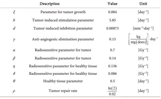
This model is completely specified by giving the values of the parameters ap-pearing in it. These values are specified in Table 1; see [6] and [8].
2.3. The Optimal Control-Treatment Problem
Usually, in the context of optimal control of cancer development models, the objective of the control is to minimize the volume of the tumor at final time, i.e.
( )
p T . See Schättler and Ledzewicz [3] for a detailed discussion of this setting. Now, while we keep this objective, we introduce additional terms that include a reduction of the tumor volume p along the time evolution, and L2- and L1-norms
of the controls u and w. With respect to the side effects of anti-angiogenetic medi-cine and radiotherapy, it is reasonable to have penalty terms for the corres-ponding controls.
We define our optimal control problem with anti-angiogenesis and radiothe-rapy as follows
(
) (
)
(
)
( )
( )
22( ) 1( ) 22( ) 1( )2 2
0, 0, 0, 0,
0
min , , , ,
: d
2 2 2 2
T u w
u w
L T L T L T L T
J p q r u w
p t t p T ν u u ν w w
σ ϑ µ µ
=
∫
+ + + + + [image:6.595.206.540.522.728.2](7)
Table 1. Model parameters.
Description Value Unit
ξ Parameter for tumor growth 0.084 [day−1]
b Tumor-induced stimulation parameter 5.85 [day−1]
d Tumor-induced inhibition parameter 0.00873 [mm−2∙day−1]
γ Anti-angiogenic elimination parameter 0.15 (kg ) day1 mg does
−
⋅
α Radiosensitive parameter for tumor 0.7 [Gy−1]
β Radiosensitive parameter for tumor 0.14 [Gy−2]
η Radiosensitive parameter for healthy tissue 0.136 [Gy−1]
δ Radiosensitive parameter for healthy tissue 0.086 [Gy−2]
θ Healthy tissue parameter 0.5 [day−1]
ρ Tumor repair rate ln 2
( )
DOI: 10.4236/am.2018.98067 991 Applied Mathematics subject to
(
)
(
)
(
)
2 4 2
3 3 3
ln ,
1 ,
,
p
p p r pw
q
q bq dq bp dp q qu r qw
r r w
ξ α β
κ κ γ η δ
ρ = − − + = − + − − − − + = − + (OCAR3)
with the initial conditions
( )
0 0, 0( )
0, 0( )
0,p = p q =q r =
and the Lebesgue measurable functions u
( )
⋅ and w( )
⋅ take their values in[
0,umax]
and[
0,wmax]
, respectively.The parameters σ ϑ ν µ ν µ ≥, , , , ,u u w w 0 can be chosen differently to obtain
different settings. We refer to this optimal control problem as the (OCAR3) control problem. Notice that in [9] a similar model is considered where only the tumor volume at the final time enters in the controls’ objective.
3. Analysis of the Anti-Angiogenesis and Radio-Therapy
Model
In this section, we analyse our cancer development and treatment differential system in (OCAR3). We have the following lemma.
Lemma 1 The model (6) with κ∈
[ ]
0,1 and u w= =0 has the equilibriumpoints
(
p q r1, ,1 1) (
= 0,0,0)
and(
p q r2, ,2 2) (
= p q, ,0)
with3 2 b p q d = = . Proof. Consider
ln p 0 0
p p p q
q
ξ
− = ⇒ = ∨ =
(
)
2 4 2
3 3 1 3 0
bq dq bp dp q
κ − + −κ − =
0 0
r r
ρ
− = ⇒ =
From the second equation with q p= , we obtain
2 2 2 2
3 3 0 3 0 0 3 0.
p b dp − = ∨p b dp − = ⇒ p q= = ∨b dp− =
Altogether, we have
3 2
0 b
p q p q
d
= = ∨ = = and r=0. □
To show that the equilibrium point
(
p q, ,0)
is locally asymptotically stable, we set z: ln= p, y: ln= q and obtain(
)
( )
(
)
( )
1 2 : , , 2exp exp : , .
3
z z y f z y
z
y b z y d f z y
ξ = − − = = − − =
(8)
DOI: 10.4236/am.2018.98067 992 Applied Mathematics
ln
z= p and y=lnq. We do not consider the third equation for r, because r is not relevant for our analysis since it neither appears in the p or the q equations, nor does p or q appear in the equation for r. Notice that the r-equation is asymptotically stable.
Using Taylor expansion, we obtain the following Jacobi matrix
( )
( )
1 1
2 3
2 2
, , 2 .
e e e
3
z
f z y z y
f f
z y
A z y z y
f f b d b
z y ξ ξ − − ∂ ∂ − ∂ ∂ = = ∂ ∂ − − ∂ ∂
At the equilibrium point
(
z y,)
, we obtain(
)
23
, 2 e .
e 3
z
f z y
A z y
b d b
ξ ξ − − = − −
We have that the trace is trA z yf
(
,)
= − − <ξ b 0 and the determinant is(
)
2 23det , e 0
3
z f
A z y = d > . Since the trace is the sum of the eigenvalues and the determinant is the product of the eigenvalues of Af, we conclude λ λ1+ 2<0 and λ λ >1 2 0. That implies λ λ <1, 2 0, hence the equilibrium point
(
z y,)
is locally asymptotically stable.Next, we show that the solution to (6) with u w= =0 is always non-negative, if the initial values are non-negative. From a medical point of view this is rea-sonable, because it makes no sense to have negative volumes and capacities. Also values for p and q that are larger than the equilibrium point
(
p q,)
cannot be reached according to the stability discussion above. On this account, we restrict our examination to the following domain(
)
{
}
(
)
3 2
2 2
, | 0 , 0 , | 0 , b .
p q p p q q p q p q
a
= ∈ < < < < = ∈ < <
(9)
Next, we consider the uncontrolled case with
κ
=1 and neglect the equationfor r since in this case r is not coupled to the
(
p q,)
-system. We haveln p
p p
q
ξ
= −
2
2 4 2 2 2 3
3 3 3 1 d 3 3 1 q .
q bq dq bq q bq
b q = − = − = −
The equation for q does not depend on p, hence q grows (independently of p) until q q= (equilibrium point) is reached. As we start with initial values
(
p q0, 0)
∈ with p0<q0, the tumor volume initially grows until p q= , but since q is growing (independently of p), we will again have p q< and the tu-mor continues to grow until p p q q= = = (equilibrium point) is reached. Hence in this case a solution that starts in will never leave .DOI: 10.4236/am.2018.98067 993 Applied Mathematics
0
κ= . Consider the following problem
(
)
(
)
2 3 ln , , . pp p r pw
q
q bp dp q qu r qw
r r w
ξ α β
γ η δ
ρ = − − + = − − − + = − + (10)
Theorem 1 The set is positively invariant for the system (10).
Proof. We show that if
(
p q0, 0)
∈ and u w, are arbitrary admissible con-trols defined on some interval[ ]
0,T , then the solution(
p( ) ( )
⋅ ,q ⋅)
with the initial condition(
p( ) ( )
0 , 0q)
=(
p q0, 0)
exists for all t∈[ ]
0,T and( ) ( )
(
p t q t,)
∈.Consider r= −ρr w r+ , 0
( )
=0. Because of w∈[
0,wmax]
, the unique solution exists and is given by( )
( )
( )0 e d 0.
t t s
r t = w s −ρ − s≥
∫
On the boundary set
{
(
p q,)
∈:p p= , 0< <q q}
, we have
(
)
0 1
ln p 0,
p p r pw
q
ξ α β
> >
= − − + <
thus the vector field points into .
Now, we look at the boundary set
{
(
p q,)
∈: 0< <p p q q, =}
. Note that the nullclines for q=0 are given by(
)
(
)
2 3
, : bp ,
q E p r
dp r
νω
γν η δ ω
= =
+ + +
for the constant controls u=ν and w=ω. We rewrite the q-equation as fol-lows
(
)
(
)
(
)
(
)
2 3 2 3 0 , .q bp dp q uq r qw
Eνω p r q dp dp q q r q
γ η δ
γν η δ ω
> = − − − + = − − − − +
We obtain that q>0 for q E< νω
(
p r,)
and q<0 for q E> νω(
p r,)
.Eνω is strictly increasing for fixed r with Eνω
( )
0,r =0 and(
,)
(
b)
.E p r p p
b r
νω = +γν+ η δ ω+ ≤
Therefore, for all p with 0< <p p , all constant controls ν∈
[
0,umax]
,[
0,wmax]
ω∈ and for every r≥0, we have
(
,)
(
,)
.Eνω p r <Eνω p r ≤ =p q
DOI: 10.4236/am.2018.98067 994 Applied Mathematics On the coordinates axes for p=0 and q=0 the dynamics has singularities,
in the sense that pln p
q
ξ
−
is not defined. Therefore, we consider the lines p xq= for x=0. Now, it is sufficient to show that x is positive for small
0
x> as follows
( )
(
)
( )
(
)
2 3 d ln d ln 0 px x x x bx dp u r w
t q
x x bx
ξ γ η δ
ξ
= = − − − − − +
> − − >
for x small enough. On the other hand, x is negative for large x
[ ]
[ ] 2
3
max 0, max
0, max max max max 1 0 r T r T
x x bx dp u r w
r
bx u w x
b b
γ η δ
η δ γ
∈
∈
< − + + + +
+
= + + − <
for
[ ]0,
max max
max
1 r T r .
x u w
b b
η δ
γ + ∈
> + +
Notice that maxr∈[ ]0,T r exists, because as we discuss below, our differential equation has an absolutely continuous solution. Hence, the region is posi-tively invariant for system (10). □
Now, let us again look at the system (6) with u w, =0. We take a closer look at the q-equation given by
(
)
2 4 2
3 3 1 3 .
q=κbq −dq + −κ bp dp q−
For initial values in the solutions to this equation with κ=0 or
κ
=1are positive and tend to zero as the equilibrium point
(
p q, ,0)
is reached (see Lemma 1). Since q is the linear combination for 0< <κ 1, it is also positive and tends to zero as the equilibrium is reached. The p- and r-equations do not depend onκ
and therefore we can deduce that for initial values(
p q r0, ,0 0)
∈ ×{ }
0 the solution cannot be negative for an arbitrary κ∈[ ]
0,1 .The model is well defined and by applying Caratheodory’s Theorem (see for example [10], Theorem 54 Proposition C.3.6) one can show existence and uni-queness of a solution to (6).
4. Optimal Solutions and the Pontryagin Maximum Principle
In this section, we discuss existence of optimal controls and their characteriza-tion by optimality condicharacteriza-tions.The existence of an optimal solution to the (OCAR3) control problem can be shown as follows. We know that all solutions x=
(
p q r, ,)
to (6) are in( )
2 0, : 0 , 0 , 0 wmax
X =x L∈ T ≤ ≤p p ≤ ≤q q ≤ ≤r ρ
DOI: 10.4236/am.2018.98067 995 Applied Mathematics
(
) ( )
[
]
{
2}
max
: 0, : 0,
ad
u U∈ = u L∈ T u t ∈ u and
(
) ( )
[
]
{
2}
max
: 0, : 0,
ad
w W∈ = w L∈ T w t ∈ w . The set X U× ad×Wad is weakly
sequen-tially compact (see [11] Theorem 2.11). As our objective J X U: × ad×Wad →,
(
x u w, ,)
J x u w(
, ,)
is convex and continuous (see [12] Theorem 2.14) and thus weakly lower semicontinuous (see [11] Theorem 2.12). Therefore we apply the direct method in calculus of variation and obtain the existence of an optimal solution to our problem (OCAR3).Next, we discuss the characterization of optimal solutions in the framework of the Pontryagin maximum principle (PMP). For this purpose and for ease of ex-position, we consider a general controlled differential model and control setting with the following properties. We have
1) An open and connected state space M ⊆n. 2) A control set U⊆m.
3) The controlled dynamical system
(
, , ,)
x f t x u= (11)
is given by the function f : 0,
[ ]
T M U× × →n,(
t x u, ,)
f t x u(
, ,)
. We assume that the partial derivative f t x u(
, ,)
x ∂
∂ is continuous as a function of all variables. 4) The class of admissible controls is taken to be a set of piecewise conti-nuous functions u defined on a compact interval
[ ]
0,T ⊆ with values in the control set U.Definition 1 The pair
(
x( ) ( )
⋅ ,u ⋅)
is called admissible if it is a solution to thedifferential Equation (11) and if u t
( )
∈U for all t∈[ ]
0,T .The objective of the control u∈ is to minimize the following functional
( )
, : 0T(
,( ) ( )
,)
d(
( )
)
.J x u =
∫
L s x s u s s g x T+Where g:n→ is continuously differentiable and L: 0,
[ ]
T M U× × → is continuous in(
t x u, ,)
, differentiable in x for fixed( )
t u, ∈ × U, and the de-rivative with respect to x is continuous.Our optimal control problem is now given as follows
( )
(
( ) ( )
)
(
( )
)
( ) ( )
(
)
( )
( )
[ ]
0
0
min , , , d
s.t. , , , 0 ,
0, .
T
J x u L s x s u s s g x T
x f t x t u t x x
u t U t T
= +
= =
∈ ∀ ∈
∫
(12)
Notice that the optimal control problem (OCAR3) that was introduced in Sec-tion 1 is of this form.
Definition 2 The Hamiltonian function H: × n× n× m→ for the
optimal control problem (12) is defined as follows
(
)
(
)
T(
)
0
, , , , , , , ,
H t x u
λ
=λ
L t x u +λ
f t x u with λ ∈0 and λ ∈n.gene-DOI: 10.4236/am.2018.98067 996 Applied Mathematics rality. This situation is called normal extremal lift; see [13].
Theorem 2 (Pontryagin’s maximum principle) Let
(
x*( ) ( )
⋅ ,u* ⋅)
be admiss-ible for the optimal control problem (12). If(
x*( ) ( )
⋅ ,u* ⋅)
is optimal, then in every point t∈[ ]
0,T in which u*( )
⋅ is continuous, we have( ) ( ) ( )
(
, * , * , *)
min(
, *( ) ( )
, * , ,)
u UH t x t λ t u t H t x t λ t u
∈
= (13)
where
λ
*( )
⋅ is the solution to the adjoint equation( ) ( ) ( )
(
)
* , * , * , * .
x
H t x t t u t
λ = − λ
For a proof see ([14], 2.4.2).
By applying PMP to our optimal control problem (OCAR3), we obtain the following necessary conditions for an optimal solution.
Proposition 3 Let
(
(
p q r*, ,* *) (
, u w*, *)
)
be an optimal solution to (OCAR3). Then in every point t∈[ ]
0,T in which(
u*( )
⋅ ,w*( )
⋅)
is continuous, we havethat the Hamiltonian
(
) (
)
(
)
(
)
( ) (
) (
)
(
)
(
(
)
)
(
)
2 2 2
1
2 1 2 2 3
, , , , , ,
ln
2 2 2
1 ,
u w
u w
H t p q r u w
p
p u w u w p r pw
q
M q M p q qu r qw r w
λ
ν ν
σ µ µ λ ξ α β
λ κ κ λ γ η δ λ ρ
= + + + + − + +
+ + − − + + + − +
at
(
t p q r, , , ,* * * λ*)
is minimized by(
u w*, *)
in[
] [
]
max max
0,u × 0,w , where
( )
*
λ
⋅ is the solution to the adjoint equation(
)
(
)
( )
( )
( )
(
)
( )
(
)
1 *
* * * * * * * 3 *
1 1 * 2
1 1
*
* * * * 3 * 3
2 1 * 2
2
* 3 * * *
* * * * * * * *
3 1 2 3
2 ln 1 3 2 4 3 3 1 p
p r w b d p q
q
p b q d q
q
d p u r w
p w q w
λ σ λ ξ ξ α β λ κ
λ λ ξ λ κ
κ γ η δ
λ λ β λ δ λ ρ
− − = − + + + + − − − = − − − + − − − − + = + + (14)
with the terminal conditions
( )
( )
* *
1 T p T
λ
=ϑ
( )
*
2 T 0
λ
=( )
* 3 T 0.
λ
=5. Numerical Optimization
DOI: 10.4236/am.2018.98067 997 Applied Mathematics for benchmarking our SQH scheme.
The main idea of the SQH scheme is the straightforward pointwise minimiza-tion of the Hamiltonian funcminimiza-tion in a way that has been first proposed in [16] [17]. Notice that, in this approach, the pointwise update of the control is per-formed on all grid points and only thereafter the corresponding state is com-puted. However, this pointwise update of the control may result in large changes of the value of the state variable that makes the proposed approach less robust. This problem is also discussed in [16] where this issue is left open. On the other hand, we have the quadratic regularisation method proposed in [18], where the Hamiltonian function is augmented with a weighted quadratic term that pena-lizes deviations from the previous control value to keep the updates of the con-trol sufficiently small. Further, in [18] every pointwise update of the control is followed by a global update of the state variable, which makes this approach very time consuming. In the SQH scheme, we combine the advantages of the two schemes performing a pointwise update of the augmented Hamiltonian on all grid points and recalculating the state variable after the control update. The augmented Hamiltonian is given by
(
) (
) (
)
(
)
(
) (
)
(
)
(
(
( ) ( )
)
2(
( )
( )
)
2)
ˆ ˆ , , , , , , , ,
ˆ ˆ
: , , , , , , ,
K t p q r u w u w
H t p q r u w u t u t w t w t
λ
λ
= + − + −
where >0 and 3 3 0
:
K +× × × × →U U
with U=
[
0,umax] [
× 0,wmax]
. We remark that by increasing a sufficient descent of the cost functional in each iteration can be achieved, see ([19], Lemma 4.1).While we refer to [19] for a detailed analysis of convergence of the SQH scheme, in the following algorithm we present the implementation of this me-thod. For this purpose, we denote x:=
(
p q r, ,)
and v=(
u w,)
.Algorithm 1 (SQH method)
1) Choose >0, κˆ 0> , σˆ 1> ,
ζ
ˆ∈( )
0,1 , ηˆ∈(
0,∞)
, v0, compute x0 from (10) corresponding to v0 and λ0 from (14) corresponding to x0 and0
v , set k←0.
2) Minimise K pointwise
(
)
arg min , , , ,k k k .
v U
v K t x λ v v
∈ =
3) Calculate x from (10) corresponding to v and calculate
( ) ( )
2 2
2 2
0, 0,
ˆ : k k
L T L T
u u w w
τ
= − + − .4) If
( )
,(
k, k)
> ˆ ˆJ x v −J x v −
ητ
: Choose ←σˆElse if
( )
,(
k, k)
ˆ ˆJ x v −J x v ≤ −
ητ
: Choose ←ζˆ, xk+1←x, vk+1←v, calculate 1k
λ + from (14) corresponding to xk+1 and vk+1 and k← +k 1. 5) If τ κˆ< ˆ: STOP and return vk.
DOI: 10.4236/am.2018.98067 998 Applied Mathematics We remark that the update of v=
(
u w ,)
is given by( )
2( ) ( )
( )
max
2
min ,max 0, ,
2
u u
t q t u t
u t = u −µ +λ ν γ +
+
( )
1( )
(
( ) ( )
2( )
(
( )
)
( )
3( )
( )
)
max2
min ,max 0, .
2
w
w
t r t p t t r t q t t w t
w t = w −µ +λ α β+ +λν η δ+ −λ +
+
To benchmark our novel method with a well-known solution scheme, we re-mark that the numerical approximation of an optimal control problem as (OCAR3) can interpreted as a nonlinear optimization problem that can be solved by using a nonlinear programming approach; see, e.g., [20]. The way we choose to perform this task is by using the modeling language AMPL [21] and the solver IPOPT [22]. We refer to the resulting optimization framework as the IPOPT-AMPL solver.
6. Numerical Experiments
This section is devoted to the investigation of the effectiveness of our numerical optimization procedure. We present results of experiments with the (OCAR3) optimization problem solved by the SQH method given by Algorithm 1. Further, to assess the computational efficiency of our scheme, we compare results of si-mulation with those obtained with the IPOPT-AMPL solver.
For all numerical experiments of this section, we consider T=10 (unless other-wise stated) and set N=1000. The two-dimensional control, denoted by
(
u w,)
, takes values in the set U=[
0,umax] [
× 0,wmax]
with umax=15 and wmax =1. For the discretization of U we choose u =50, w=10. As initial guess for the controls, we take the zero function. Further, we initialize our state variables with0 8000
p = , q0=10000 and r0 =0. The parameters in Algorithm 1 are chosen
as κˆ 10= −7, σˆ 50= , ζˆ 0.15= , ηˆ 10= −7 and the initial guess =0.1.
For the first experiment setting, we choose additionally κ =0.5 and the L1-
and L2-penalty parameters are given by 0
u w
µ =µ = and νu=νw=1, respectively.
By using Algorithm 1 with this setting, we obtain the optimal solution showed in
Figure 2. An almost identical solution is obtained with the IPOPT-AMPL solver. The tumor volume reduces to p T
( )
=22.2847, that is, a reduction of more than two orders of magnitude of the initial volume. However, as the carrying capacity of the vasculature with q T( )
=325.253 is larger than p T( )
the tu-mor will grow again after the treatment.In Table 2, we further compare the results obtained with the SQH and IPOPT-AMPL schemes showing that the resulting values of the objective and the states at the terminal time T are similar. In both cases, the control w is a constant function taking the maximum value wmax =1 in the entire interval
[ ]
0,T . However, the SQH method only needs a 1/50 of the CPU time needed by the IPOPT-AMPL scheme.DOI: 10.4236/am.2018.98067 999 Applied Mathematics Figure 2. Optimal solution obtained with the IPOPT-AMPL and SQH schemes for the first experimental setting.
Table 2. Comparison of the results of the SQH and IPOPT-AMPL methods for the first experimental setting.
SQH IPOPT-AMPL
J 424.6 430.1
( )
p T 22.2847 22.4486
( )
q T 325.253 325.235
time 0.128 6.514
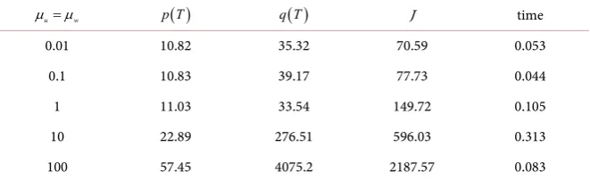
Table 3. Results for increasing L1 penalty parameters.
u w
µ =µ p T( ) q T( ) J time
0.01 10.82 35.32 70.59 0.053 0.1 10.83 39.17 77.73 0.044
1 11.03 33.54 149.72 0.105
10 22.89 276.51 596.03 0.313 100 57.45 4075.2 2187.57 0.083
rest of the setting remains as in our first example. We see, that the increase of the penalty parameters µu and µw results in higher values for p, q and J. This is reasonable since the increase of µu and µw describes higher costs for the controls.
In the second numerical experiment, we consider
κ
=1 and the L1-penaltyparameters µu=µw=0.01. The L2-penalty parameters and the other
parame-ters are the same as for the first experimental setting. With this setting and using Algorithm 1, we obtain the solution displayed in Figure 3.
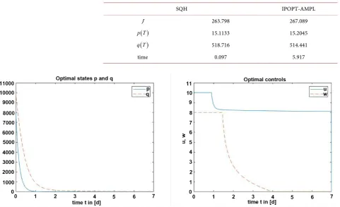
[image:15.595.208.539.443.544.2]DOI: 10.4236/am.2018.98067 1000 Applied Mathematics Figure 3. Optimal solution obtained by the IPOPT-AMPL and SQH schemes for the second experimental setting.
setting, but now the carrying capacity of the vasculature is larger with
( )
518.716q T = , so again the tumor will grow after the treatment. As above, IPOPT-AMPL provides a comparable solution and the results presented in Ta-ble 4 also confirm this fact. Again the computation time for the SQH method is less than the one needed by IPOPT.
In the experiments above, our focus was the comparison of the SQH method with the IPOPT-AMPL scheme. For this reason, less attention has been put on the ability of our optimal control formulation to deliver effective treatment. In the following experiments, we would like to show that it is indeed possible to find an optimisation setting that results in control functions that are able to re-duce the volume and carrying capacity to zero at final time. In particular, we show the importance of the L1-cost towards this task.
Indeed, control costs of L1-type are considered in the literature for their ability
to promote sparsity of controls. However, this feature is usually validated with a single control function, whereas in our case two control functions are considered that act on a nonlinear coupled system. In fact, as results of our experiment show, the choice of the weights of the costs of the control is a delicate issue.
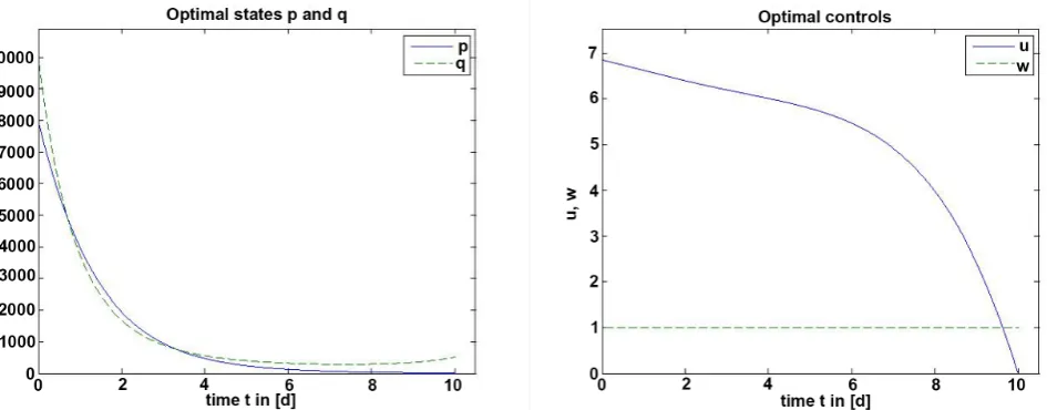
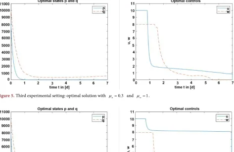
For our experiments, we choose a time horizon T=7 (7 days), and the fol-lowing control bounds umax=10, wmax =8. The other parameters are chosen as follows: σ =1, ϑ=1, κ=0.5. We focus on the L1 weights while choosing
0.01
u w
ν =ν = for the L2 costs of the controls. This is our third experimental
setting that is organised as follows.
DOI: 10.4236/am.2018.98067 1001 Applied Mathematics Table 4. Comparison of results with the SQH and the IPOPT-AMPL schemes for the second experimental setting.
SQH IPOPT-AMPL
J 263.798 267.089
( )
p T 15.1133 15.2045
( )
q T 518.716 514.441
time 0.097 5.917
Figure 4. Third experimental setting: optimal solution with µu=0.1 and µw=1.
reason, we keep all weights equal but slightly increase µ =u 0.3. The results of
this experiment are shown in Figure 5. As expected, we can see a reduction of the control function u towards zero. However, it remains non-zero, and it has the effect that the control w is less sparse. Even more important, with this setting the carrying capacity remains non-zero. This result may suggest that we should increase both µu and µw, as we do in a third experiment, choosing µ =u 1 and µ =w 6. The corresponding results are depicted in Figure 6. Notice that
this result is qualitatively similar to the first one with µ =u 0.1 and µ =w 1: we do not get a striking better result. Finally, we choose µ =u 2 and µ =w 10. In this case, the L1 weights are large enough to get sparse control functions, but this
is achieved at the cost of a non-zero and increasing carrying capacity; see Figure 7. Therefore our control framework allows to make the appropriate tuning of the optimisation weights in order to obtain promising successful treatments as with the first and third experiments.
7. Conclusions
DOI: 10.4236/am.2018.98067 1002 Applied Mathematics Figure 5. Third experimental setting: optimal solution with µu=0.3 and µw=1.
[image:18.595.60.536.289.478.2]Figure 6. Third experimental setting: optimal solution with µu=1 and µw=6.
[image:18.595.61.539.514.704.2]DOI: 10.4236/am.2018.98067 1003 Applied Mathematics To determine these therapies, an optimal control problem was formulated considering a cost functional including the tumor volume and L1- and L2-penalty
terms for the controls. After the proof of existence of minimizers, the necessary optimality conditions that characterize these minimizers were deduced in the framework of the Pontryagin maximum principle. Based on this PMP frame-work, the SQH method was used for numerical solution. This algorithm was used to solve the optimal cancer therapy problem with different experimental settings. Furthermore, optimal solutions obtained by the SQH algorithm were compared with the optimal solution obtained by the IPOPT solver together with the programming language AMPL. This comparison showed that the SQH me-thod is faster by a factor 10 than IPOPT. In a final series of experiments it was shown that it is actually possible to choose the optimisation parameters in such a way to reduce the volume of the tumor and the related carrying capacity to zero.
Acknowledgements
We thank the Referee for helpful comments and pointers to the literature. This publication was funded by the German Research Foundation (DFG) and the University of Würzburg in the funding programme Open Access Publishing.
Conflicts of Interest
The authors declare no conflicts of interest regarding the publication of this pa-per.
References
[1] Azizi, M. and Hesameddini, E. (2017) Grünwald-Letnikov Scheme for System of Chronic Myelogenous Leukemia Fractional Differential Equations and Its Optimal Control of Drug Treatment. Journal of Mahani Mathematical Research Center, 5, 51-57.
[2] Moore, H. (2018) How to Mathematically Optimize Drug Regimens Using Optimal Control. Journal of Pharmacokinetics and Pharmacodynamics, 45, 127-137.
https://doi.org/10.1007/s10928-018-9568-y
[3] Schättler, H. and Ledzewicz, U. (2015) Optimal Control for Mathematical Models of Cancer Therapies. Springer, Berlin/Heidelberg.
https://doi.org/10.1007/978-1-4939-2972-6
[4] Chudej, K., Huebner, D. and Pesch, H.J. (2016) Numerische Lösung eines mathe-matischen Modells für eine optimale Krebskombinationstherapie aus An-ti-Angiogenese und Strahlentherapie. In: Tagungsband ASIM 2016-23 Symposium Simulationstechnik, Dresden, Volume 52 of Argesim Report, ARGESIM Verlag, Wien, Austria, 169-176.
[5] Hahnfeldt, P., Panigrahy, D., Folkman, J. and Hlatky, L. (1999) Tumor Develop-ment under Angiogenic Signaling. Cancer Research, 59, 4770-4775.
[6] Ergun, A., Camphausen, K. and Wein, L.M. (2003) Optimal Scheduling of Radio-therapy and Angiogenic Inhibitors. Bulletin of Mathematical Biology, 65, 407-424.
https://doi.org/10.1016/S0092-8240(03)00006-5
Li-DOI: 10.4236/am.2018.98067 1004 Applied Mathematics
near-Quadratic Model with Incomplete Repair and Volume-Dependent Sensitivity and Repopulation. International Journal of Radiation Oncology, Biology, Physics, 47, 1073-1083. https://doi.org/10.1016/S0360-3016(00)00534-4
[8] Bellomo, N. and Preziosi, L. (2000) Modelling and Mathematical Problems Related to Tumor Evolution and Its Interaction with the Immune System. Mathematical and Computer Modelling, 32, 413-452.
https://doi.org/10.1016/S0895-7177(00)00143-6
[9] Chudej, K., Wagner, L. and Pesch, H.J. (2015) Numerical Solution of an Optimal Control Problem in Cancer Treatment: Combined Radio and Anti-Angiogenic Therapy. IFAC-PapersOnLine, 48, 665-666.
https://doi.org/10.1016/j.ifacol.2015.05.082
[10] Sontag, E.D. (2013) Mathematical Control Theory: Deterministic Finite Dimen-sional Systems. Volume 6. Springer Science & Business Media, Berlin/Heidelberg. [11] Tröltzsch, F. (2010) Optimal Control of Partial Differential Equations. Graduate
Studies in Mathematics. American Mathematical Society, Providence.
[12] Adams, R.A. and Fournier, J.J.F. (2003) Sobolev Spaces. Volume 140. Academic Press, Cambridge.
[13] Schättler, H. and Ledzewicz, U. (2012) Geometric Optimal Control: Theory, Me-thods and Examples. Volume 38. Springer Science & Business Media, Ber-lin/Heidelberg.
[14] Ioffe, A.D. and Tihomirov, V.M. (2009)Theory of Extremal Problems. Volume 6. Elsevier, Amsterdam.
[15] Mehne, H.H. and Mirjalili, S. (2018) A Parallel Numerical Method for Solving Op-timal Control Problems Based on Whale Optimization Algorithm. Know-ledge-Based Systems, 151, 114-123.
[16] Krylov, I.A. and Chernous’ko, F.L. (1963) On a Method of Successive Approxima-tions for the Solution of Problems of Optimal Control. USSR Computational Ma-thematics and Mathematical Physics, 2, 1371-1382.
https://doi.org/10.1016/0041-5553(63)90353-7
[17] Krylov, I.A. and Chernous’ko, F.L. (1972) An Algorithm for the Method of Succes-sive Approximations in Optimal Control Problems. USSR Computational Mathe-matics and Mathematical Physics, 12, 15-38.
https://doi.org/10.1016/0041-5553(72)90063-8
[18] Sakawa, Y. and Shindo, Y. (1980) On Global Convergence of an Algorithm for Op-timal Control. IEEE Transactions on Automatic Control, 25, 1149-1153.
https://doi.org/10.1109/TAC.1980.1102517
[19] Breitenbach, T. and Borzì, A. (2018) A Sequential Quadratic Hamiltonian Method for Solving Parabolic Optimal Control Problems with Discontinuous Cost Func-tionals. Journal of Dynamical and Control Systems.
[20] Betts, J.T. (2001) Practical Methods for Optimal Control and Estimation Using Nonlinear Programming. SIAM, Philadelphia.
[21] Fourer, R., Gay, D. and Kernighan, B.W. (2003) AMPL: A Modeling Language for Mathematical Programming. Pacific Grove, Duxbury/Thompson.