Algorithms for sorting nearly sorted lists

cosc

460

Department of Computer Science

University of Canterbury

Supervisor: Dr. A. Moffat

John Wright

CONTENTS

Abstract . . . 3

1.0 Introduction . . . 4

2.0 Preliminary Testing . . . 5

2.1 Sortedness Ratio . . . . . . . . . . . . . . . . . . . . . . . . . . . . . 5

2.2 Inversions . . . 6

2.3 Number of Ascending Sequences . . . 7

2.4 Longest Ascending Sequences . . . 7

2.5 Number of Exchanges . . . 8

2.6 Results . . . 10

2. 7 Conclusions . . . 11

3.0 The Implementation of Five Algorithms . . . 12

3.1 Linear Insertion Sort . . . 13

3.2 Ysort . . . 14

3.3 Cksort . . . 16

3.4 Natural Mergesort . . . 17

3.5 Smoothsort . . . 19

3.6 Results . . . . . . . . . . . . . . . . . . . 23

3.7 Conclusions . . . 25

4.0 Improvements, Modifications and Other Ideas . . . 26

4.1 Improvements to Y sort . . . 26

4.2 Improvements to Cksort . . . 27

4.3 Alterations to Smoothsort . . . 29

4.4 Alterations to Linear Insertion Sort . . . 30

5.0 Conclusions . . . 33

Appendix A . . . 34

Appendix B . . . . . . . . . . . . . . . . . . . . . . . . . . . . . . . . . . 37

Appendix C . . . . . . . . . . . . . . . . . . . . . . . . . . . . . . . . . . . . . 42

References . . . 44

ABSTRACT

The following five algorithms for sorting in situ are examined: linear

insertion sort, cksort, natural mergesort, ysort and smoothsort. Quicksort and

heapsort are also considered although they are not discussed in detail. The

algorithms have been implemented and compared, with particular emphasis

being placed on the algorithms' efficiency when the lists are nearly sorted.

Five measures of sortedness are investigated. These are sortedness ratio, number of inversions, longest ascending sequence, number of ascending

sequences, and number of exchanges. The sortedness ratio is chosen as a

basis for comparison between these measures and is used in experiments on

the above algorithms.

Improvements to cksort and ysort are suggested, while modifications to

smoothsort and linear insertion sort failed to improve the efficiency of these

algorithms.

1.0 INTRODUCTION

One of the most widely studied problems in computer science is sorting. Algorithms for

sorting were developed early and have received considerable attention from mathematicians and

computer scientists. A large number of algorithms were developed, but no one algorithm is best

for all situations and in many cases the files to be sorted are just too large and need to be sorted

externally using discs or tapes as the storage medium. In recent years the interest in sorting has concentrated on algorithms that exploit the degree of sortedness of the input.

Quicksort is an internal sorting algorithm that was first proposed by C.A.R Hoare [1] in

1962 and has been studied extensively. It has been widely accepted as the most efficient internal sorting algorithm and achieves a lower bound of O(n log n), but has a worst case complexity of O(n2) and the algorithm does not attempt to exploit the degree of sortedness of the input. Many

modifications to quicksort have occurred and there exists a large number of algorithms based on the original theme. Other algorithms such as heapsort and mergesort achieve an O(n log n) lower

bound and yet do not have quicksort's worst case complexity, but these algorithms also do not

take into account the sortedness of the input.

Considered here are five algorithms for sorting in situ. Each algorithm is claimed to have

good behaviour on nearly sorted lists. In particular linear insertion sort, natural mergesort,

ysort, cksort and smoothsort have been studied. Both ysort and cksort have utilized the

quicksort algorithm or one of its descendants. Natural mergesort is an extension of the merge

sorting technique, but uses natural runs, ascending or descending sequences, in the data.

Smoothsort is a new algorithm, proposed by Dijkstra [8] that uses a sophisticated data structure

based on heaps and was designed specifically to sort nearly sorted lists in linear time and have a

worst case complexity of O(n log n). Finally insertion sort has been included as its performance

on nearly sorted lists is widely known although it has a worst case complexity of O(n2).

All of the algorithms attempt to utilize the sortedness of the data in some way and each is

claimed to have O(n) complexity on nearly sorted lists.

2.0 PRELIMINARY TESTING

In dealing with sorting algorithms the phrases " ... on a nearly sorted list ... " and " ... on a randomly sorted list ... " arise frequently, but a list may be "nearly" sorted according to one

terminology and "randomly" sorted according to another. Intuitively a list is nearly sorted if only

a few of its elements are out of order. The problem is to define an easily computable measure

that coincides with intuition.

A list will be considered sorted if all its elements form a non decreasing sequence and a list is reverse sorted if all its elements form a non ascending sequence. A list of length n can be sorted

in O(n) time if the number of operations on all the elements of the list is proportional ton by

some constant factor. For example the list,

5 6 7 8 4 3 2 1,

can be sorted in O(n) since n/2 comparisons and n/2 swaps are needed to sort the list, provided the list is sorted by merging sequences from opposite ends.

This chapter discusses and relates five measures of sortedness, the sortedness ratio,

inversions, number of ascending sequences, longest ascending sequence and the number of

exchanges. The first measure discussed [2] provides a basis from which to compare the other

four measures. Results have been graphed and also included in Appendix A.

2.1 Sortedness ratio

Cook and Kim [2] defined the sortedness ratio of a list of length n as,\

sortedness ratio

=

kin,

where k is the minimum number of elements that need to be removed to leave the list sorted. For

a sorted list this ratio is O since all the elements are in their correct positions and for a list in reverse sorted order this ratio approaches 1. For example,

21354

has sortedness 2/5 since the removal of 5 or 4 and 1 or 2 will leave the list sorted.

This measure of sortedness is by no means perfect. Consider the following lists:

87654321 21436587

The first list has a sortedness ratio of 7/8, the maximum possible sortedness ratio for a list, yet it can be sorted in O(n) time by reversing the list. The second list contains local disorder and has a

sortedness ratio of 4/8, indicating a high degree of unsortedness. Yet it too can be sorted in O(n)

time by an algorithm that will exploit local disorder.

2.2 Inversions

For a list on n elements; x_1, x_2, x_{3, ...} xn, the number of inversions is defined to be,\

number of inversions

=

Ii=l,n-l Ij=i+l,n inv,

where inv

= {

0 if xi ~ xj, { 1 if xi > xj.

If the list is in reverse order there are n(n - 1)/2 inversions. The number of inversions is bounded below by 0, for the sorted list, and above by n(n - 1)/2, for the reverse sorted list. For

example in the list,

423865

there are 5 inversions, namely (4,2), (4,3), (8,6), (8,5) and (6,5).

This measure of sortedness indicates a list in reverse order would be less sorted than a list of

elements chosen from a random distribution. For example, in

10987654321

87531492610

the first list has 45 inversions, indicating a high degree of unsortedness but certainly can be

sorted in O(n) time. The second list contains 22 inversions but has no obvious properties that

allow it to be sorted in O(n) time.

2.3 Number of ~scending Sequences

_t

'>,

The number of ascending sequences in a list of length n is defined as,

number of ascending sequences = I,i=l,n-l (run) + 1,

where run= { 1 if xi+l <xi, { 0 if xi+l :::: xi.

For example in the list,

5 4 9 2 6 7 8 3 10 11 15,

there are 4 ascending sequences partitioned as follows,

(5) (4 9) (2 6 7 8) (3 10 11 15).

For a list in sorted order there is just 1 ascending sequence and for a list in reverse order

there are n ascending sequences. This method has its disadvantages in lists which have a high

degree of local disorder. For example, lists such as,

2 1 4 3 6 5 8 7 ... ,

have a large number of ascending sequences but certainly have properties that allow linear time

sorting since each element is only one position from its correct position in the sorted list.

2.4 Longest Ascending Sequence

The longest ascending sequence of a list can be seen from the following example,

1541236798

which is partitioned into the following ascending sequences,

(1 5) (4) (12367 9) (8),

with the longest ascending sequence of length 6.

A sorted list has a single ascending sequence of length n and a reverse sorted list has n

ascending sequences of length 1 and generally the greater the number of ascending sequences

the less sorted the list. But consider the following lists:

21436587109

10987654321

10563582174

Both the 1st and 2nd lists have immediate properties that allow O(n) time for sorting. In the first

list each element is 1 position from its sorted position, even though the longest ascending

sequence is of length 1. The 3rd list has no obvious properties yet its longest ascending sequence is of length 3, and according to this measure it is more sorted than the first two lists.

2.5 Number of Exchanges

The number of exchanges in a list is the smallest number of exchanges of elements needed to

bring the list into a sorted order. For example the list,

13879546,

requires 3 exchanges to move the elements into their correct position:

1 3

.a

7 9 5

.4

6 1 3 4

₁

9

5.

8 6 1 3 4 5

_.2.

7 8 .Q

1 3 4 5 6 7 8 9

A sorted list clearly requires O exchanges, on the other hand a reverse sorted list requires [n/2J exchanges.

Since each exchange will move at least 1 element into its correct place there will be at most

O(n) exchanges required to construct the sorted list. For example in the list,

5 1 2 3 4,

n-1 or 4 exchanges are required to sort the list as follows.

page8

·-5.

1

2 3 4

1

5.

2

3 4

125.:14

1 2 3

5.

~

1 2 3 4 5

One of the disadvantages of this measure can be seen in the above example which required the

maximum number of exchanges to sort the list, indicating a high degree of unsortedness, but the

list can certainly be sorted in O(n) time by swapping the first element into the last position of the

list.

The main disadvantage of this measure is illustrated in figure 4 and shows that the number of

exchanges does not correlate well with the sortedness ratio and other sorting measures

compared. Consider a sorted list of length n. If just one element is removed and inserted at a

random position elsewhere in the list then the average distance between the element's new

position and its correct position will be 1/3n. O(n) or l/3n exchanges will be required to move

the element to its correct position, so_ a sortedness ratio of 1/n will have l/3n or O(n) exchanges.

As n increases 1/n becomes a smaller fraction but will still result in O(n) exchanges, whereas a

list with a smaller sortedness ratio should require less effort to sort.

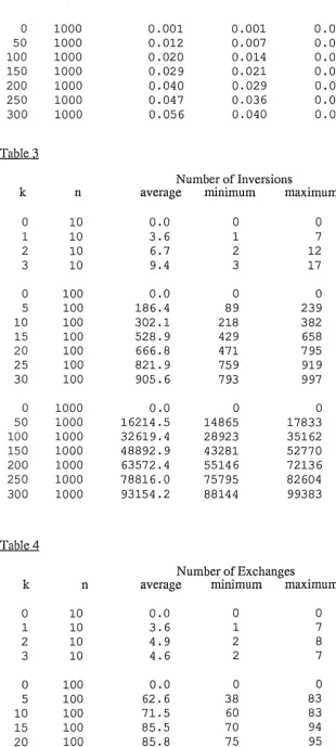
2.6 Results

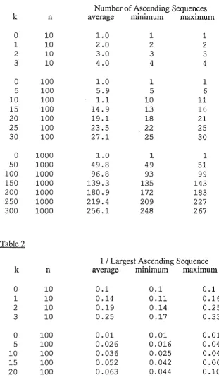
Experiments were run on lists of length 10, 100 and 1000. The lists were generated by first

taking a sorted list and removing k elements, from random positions within the list, and then inserting these k elements at new random positions within the list. If the inserted elements

formed an ascending sequence with its two adjacent elements then it was shifted either left or

right to ensure the list had a sortedness ratio of kin. The sortedness ratio was varied between 0%

and 30% and for each list generated the number of inversions, ascending sequences, exchanges

and the longest ascending sequence was determined. Results obtained were graphed, the point

graphed being the average of 10 trials. Results have also been included in Appendix A along

with the maximum and minimum values for each trial.

Of particular interest was the relationship with other measures of sortedness when the list

was nearly sorted. Further analysis showed that as the sortedness ratio became higher than

30%, the first two measures considered, number of inversions and number of ascending sequences, began to approach an upper bound asymptotically. This can be seen in figures 1 and

2 where a linear line has approximated the points plotted, but as the sortedness ratio has increased the points have fallen below the line plotted.

It can be seen from the graphs that the first three measures considered correlated successfully with the sortedness ratio. The number of inversions, figure 1, increases quadratically as the

sortedness ratio increases, but a linear relationship has been obtained when the number of

inversions have been scaled by l/n2. The number of ascending sequences, figure 2, gives a

good linear approximation especially when the sortedness ratio is small, but as the sortedness

ratio approaches 25% this relationship begins to deteriorate. The inverse of the longest

ascending sequence, figure 3, has the closest relationship with the sortedness ratio and the

deterioration in the linear correlation was not apparent as the sortedness ratio was varied from

0% to 30%. The last measure considered, number of exchanges, shows a poor correlation with

the sortedness ratio for reasons explained in 2.5. As n increases the number of exchanges more

rapidly approaches the upper bound of n-1 exchanges.

C,0

Q.12

0,11

0.10

0.09

C\lc 0.08

~

om

.Q VJ

tJ

C).06

>

c

4--

0.05

0

L

1s

o.04

E

::J

Z a.OJ

-·-·-·-·-· ---.---_{·.-.-_-::..-:} --... ::;~/-::~

n

~

the length of the list

0.1 _Q,2

.So

c.

tedness

Ratio

I I

n

=

the length of the list

Sortedness Ratio

n

=

the

length

of the

list

l\:i'IOO

0.1

Sortedness Ratio

,

fiigure

3.

Sortedness

Ratio

and

the Largest Ascending

Sequence.

( ... .::·.-"..·

I ..

C,ORMACI ( n n p PE n ( t r

l

ll

{ I

l]IT

_I

_ljj!

+

~, I

_$

f

_I

Hi

! 1: : ',I 'lj l I It

l

:j

111

11

:r J

I I

i=r,

l"l

I i

ltl _I

_ji

_I

..

,I

ij

ii 1, " 11!

I

_{j1 I}

_I

:c CL

I' I _I 1

1 1! I,

I

1

il

:I

i

!

r

~

·~

~-I~

t

+

ll

11 11 ' t ,

1

_

I

'I

!l

1

?

11 I, JI

11

ill

l i

," lj

_n

I,-++ tt

I

I

t'

! I

Iii

r

I I Ii 11! _t

I!

I~!

Ill

I, +

1.0

,11

T

+

1_{1 I r}

I 111

It

o.9

1111 ,

''\I

1

o.S

It

I

1, 1 I

i

J

,II

It

o.1

!11 i

I I : c

11: ,,i,

iii I•:

---I'' U) _0.6

"

11 \ (lJ

ii!

!

en c

it!!

!

ro _().$ ..c

1,11 I u x

II

!t

w

II, _OA !

~i

~

I

!

l....

(lJ

0.3 I

..0

E:

I

' :t _:0 '

I

z

O.?,'

I

I

, ,

'\:

v

:11 : 1:.1 _'0.1

! ' I

~I,

1Ht 11:i

+I-rl, 1••

I I ' ! I J

r

'lj!

t

i1l _~-0

j

I

If

I''

t

t ,++ •

t

~:

'

t

t

I

I

' l_

' !

-t-+

=

the

length

of

the list

0.1

Sortedness

Ratio

I

J I

j:

1

t

1J1 I

11

111 + j

II Ji

'if

I

\

Fj

i

g

u~

~

~

+

Ii

!1H

t

r

jl

*

I t

'Ji

E l , .,

rJ

Ir f

i

I

d

!

/i

+

t

~+ t

r·

+I

i l ' ! I

1

,-:. , H:, rt. ::It _l

4.

Sortedness

Ratio

and

the

Nurn\Jer

of

Exchanges.

+

I .

I

I.

2.7

Conclusions

The problem still remains to find a measure of sortedness that returns appropriate values for

all lists that have properties that allow O(n) sorting. For the measures discussed here, a list may

be nearly sorted by one measure and very unsorted by another.

Algorithms that have been claimed to give good performance on nearly sorted lists have

typically been tried on lists in which the measure of sortedness has been the measure that the

algorithm best exploits. For example natural mergesort utilizes the natural runs, ascending or

descending sequences, and compared with alternative algorithms, gives good results on lists

which contain a high percentage of runs. Insertion sort performs well on list that have a high

degree of local disorder, for example sequences of the form,

2, 1, 4, 3, 6, 5 ...

This type of sequence has a low number of inversions but is almost totally unsorted according to the other measures discussed.

3.0 THE IMPLEMENTATION OF FIVE ALGORITHMS

Five algorithms, linear insertion sort, ysort, cksort, natural mergesort and smoothsort, were

chosen and implemented in Pascal and run on a Prime 750 at the University of Canterbury.

These algorithms have been chosen as their authors have claimed they have good performance on nearly sorted lists, although in many cases a precise definition of a nearly sorted list has not

been given, and justification for the algorithm's efficiency has only been provided by way of

worked examples or a general discussion of the algorithms behaviour.

In addition to these five algorithms, quicksort and heapsort have been implemented. Quicksort is generally accepted as the best internal sorting algorithm and is often implemented as

a system sort. It has been implemented here as a hybrid algorithm with linear insertion sort and uses the middle element as the partition element [3]. Heapsort was included as its worst case and

average case complexity is O(n log n), unlike quicksort which has an O(n2) worst case

complexity. For this reason heapsort is often implemented in situations where the sorting time of

an algorithm is critical, since its O(n log n) behaviour can be guaranteed.

3.1 Linear Insertion Sort

The simplest of the algorithms implemented was linear insertion sort [ 4]:

begin

i := 2;

while i ::;;; n do begin

j := i;

while j > 1 cand A[j] < A[j-1] do begin

swap(A[j],A[j-1]);

j := j - 1;

end;

i := i + 1;

end;

end

The simplicity of this algorithm makes it very useful and for small values of n it is frequently

implemented, even if the structure of the list is unknown.

The algorithm has an O(n2) worst case complexity, but on lists in which each element is no

more thank positions from its final position it has an O(kn) complexity. This fact makes it very

useful for a sorting algorithm on nearly sorted lists and also makes it very useful in hybrid

algorithms. For example, Sedgewick [3] used insertion sort to very good effect in a hybrid algorithm with quicksort.

3.2 Ysort

Ysort [5] is a variation on the quicksort algorithm. Its main difference from quicksort occurs

in the construction of the sublists as shown in the following description of the algorithm.

Unsorted array is in A[l .. r], initially l is 1 and r is n.

begin

i, j, T := 1, r, partition element

while i <= j do begin

while A[i] < T do begin

i := i + 1

get position of minimum and maximum values of left subfile, A[l .. i] end;

while A[j] > T do begin

j := j - 1;

get position of minimum and maximum values of right subfile, A[j .. r] end

i, j, A[i], A[j] := i+l, j-1, A[j], A[i)

get positions of minimum and ~aximum values for left and right subfiles end

swap minimum and maximum values into position, if necessary

if left subfile not sorted then sort the sublist A[l+l] .. A[j-1) if right subfile not sorted then sort the sublist A[i+l] .. A[r-1)

end

As the sublists are constructed the location of the minimum and maximum elements of each

sublist are recorded. When the partitioning step is completed the minimum and maximum

elements are exchanged with the left and right elements of each sublist respectively. Ysort is

then used again to sort the left and right sublist. The new sublists to be sorted exclude the end

elements as these are the minimum and maximum elements and are now in their correct position.

After a partitioning step on an unsorted array, A[l..r], the array will have the following

properties.

11 ::::; T

l

subfile to l>e sorted

m. iD.im. 'U.Ill. Thlue of Mt subfile

j i r

I I I

~T 11

l l

,.i,m,

to ) t " " ' '

l

m.~ 'U.Ill.

ruv.e

m.i.D.im. 'U.Ill.

ruv.e

m.~ 'U.Ill.

ruv.e

of ~ft subfile of right subfile of right subfile

T :is the value of the p arti.tion element.

The advantage with this algorithm is that it also keeps track in the construction of each sublist

whether the new element placed in the sublist is the new maximum element for the left sublist or

the new minimum element for the right sublist. If for the left sublist each new element placed in the list becomes the new maximum element then the list will be sorted and needs not be partitioned any further. A similar argument applies for the right sublist. For a nearly sorted list

ysort needs only to partition until it finds a sorted sublist. Since there will be many sorted

sublists in a nearly sorted list few partitioning steps will be required to sort the list completely.

The cost of this algorithm compared with quicksort is the additional number of comparisons

it needs to make to keep track of the maximum and minimum elements of each sublist.

3.3 Cksort

Cksort as proposed by Cook and Kim [2] is essentially a hybrid sorting technique based on three sorting algorithms: quicksort, linear insertion sort and merging. Like all hybrid algorithms

it attempts to exploit the advantages of each of its composite algorithms.

A is the unsorted list, Bis used for processing.

begin

first, second, place, upto := 1, 2, 1,1 while second<= n do

begin

if A[first] > A[second] then begin

B[place], B[place+l], place := A[first], A[second], place+2

first, second:= previous element compared, next uncompared element end

else begin

A[upto], A[upto+l] := A[first], A[second]

first, second, upto := upto+l, second+l, upto+2 end

end

if place -1 > 30 then

quicksort B[l] .. B[place-1] else

- number of elements in list B

insertion sort B[l] .. B[place-1]

merge list A[l] .. A[upto-1] and B[l] .. B[place-1] end

The first pass of cksort scans the list and removes all unordered pairs of elements and places

them in a separate list. After a pair of unordered elements has been removed, the next pair

compared are the elements immediately preceding and immediately following the pair just

removed. Upon completion of the first pass the original list will be sorted since it contains only

ordered pairs. The second list, of unordered pairs, is then sorted by either quicksort if there is

more than 30 elements or by inse1iion sort, otherwise. Finally the two sorted lists are merged.

For a nearly sorted list there will be few unordered pairs removed, which are then sorted

efficiently by either quick sort or linear insertion sort and merged with the first list. The removal

of unordered pairs in a nearly sorted list will take O(n) time, the sorting of the small number of

unordered pairs will be efficiently perf01med by quicksort or linear insertion sort, and finally the

merging with the first list will take O(n) time, giving the algorithm a complexity of O(n) on a

nearly sorted list. For an unsorted list, the list will consist of mostly unordered pairs which will

be placed in the second list to be sorted by quicksort. In this case the algorithm deteriorates to

the average case complexity of quicksort, namely O(n log n).

3.4 Natural Mergesort

Natural mergesort is described by Knuth [6] and takes advantage of the runs, ascending and

descending sequences, within a list. The algorithm merges runs from opposite ends of the

unsorted list, the merged sequences being placed at alternate ends of a separate list. When all

runs from the first list have been merged the separate list will contain half the number of runs as

the first. The separate list is then processed in a similar manner to the first until eventually a list

contains only one non decreasing sequence.

listl contains the unsorted list list2 is the list used in processing

begin

number of runs := n - some arbitrary value> 1 lista, listb := listl, list2

while number of ascending runs> 1 do begin

1, r := 1, n while l <= r do

begin

merge ascending sequence starting at l with the ascending sequence (right to left) starting at r put merged sequence in opposite end of listb

l := next ascending sequence from left r := next ascending sequence from right end

listb, lista := lista, listb end

if listb = list2 then

listl := listb

end

- copy unsorted array to sorted array

If the list is nearly sorted there will be few passes, but on a random list there will be about 1/2n runs, resulting in O(log n) passes, since each pass halves the number of runs. For each

pass there will be O(n) comparisons giving the algorithm an average case and worst case

complexity of O(n log n).

In the following example the arrows indicate the natural runs in the list. Each pass merges

natural runs from opposite ends placing the merged sequences at alternate ends of the new list.

E E ~

-503 087 512 061 908 170 897 275 653 426 154 509 612 677 765 703

--;>----> - - - - > ---3> - - - - ' ; ) ,

<; ~ ~ -503 703 765 061 612 908 154 275 426 653 897 509 170 677 512 087

---,> - - - ' ; ) ,

- - -

----:>

E ~

-087 503 512 677 703 765 154 275 426 653 908 897 612 509 170 061

---> ---

>

<---061 087 170 503 509 512 612 677 703 765 897 908 653 426 275 154

---~---~--- a>

~-061 087 154 170 275 426 503 509 512 612 653 677 703 765 897 908

~--->

3.5 Smoothsort

Smoothsort is a sorting algorithm proposed by Dijkstra [8][9]. It attempts to address the problem of sorting nearly sorted lists with O(n) complexity while retaining a worst case complexity of only O(n log n), and to provide a smooth transition between the two. The

implementation of the algorithm has also been described by Hertel [10], with a slight variation

on Dijkstra's proposal. However the asymptotic behaviour of the algorithm remains the same. Hertel's description is easier to analyse and implement and was chosen as the algorithm to be

coded and explained.

begin

while elements still remaining do begin

k := llog2(number of remaining elements) I

Make a complete heap of the 2k-1 remaining elements. Swap the new root leftwards until the

roots form a non decreasing sequence. Sift the root into its correct place in the heap. end

m := n

while m > 1 do begin

if size of last heap is 1 then

Remove the heap from consideration,

element is in its correct position. else

begin

Remove the root form consideration, the root element is in its correct positionand split the remainder of the heap into two heaps of equal size.

Swap new roots leftwards so that the

roots form a non decreasing sequence.

Sift the new roots into their correct place within their heaps. end

m := m - 1

end

- one more element in its correct place

end

The algorithm uses a sophisticated data structure based on heaps and consists of two passes.

The first pass builds a forest of complete heaps. Each of the heaps constructed has 2k-1

elements, k ~ 0, so each element of the heap has either O or 2 sons. The first heap is as large as possible and will contain at least half the elements of the list. Successive heaps are of decreasing

size. The exception to this rule occurs for the last two heaps constructed which may be of the

same size. The root of each heap is at the right most position of the elements of the heap. Each

heap is constructed over A[i .. j] so that a root at position j has sons at position j-1 and at position

_ i + (j-1) div 2 - 1.

For example, in an array of size 28 the size of the heaps constructed will be 15,7,3 and 3, the

roots of each heap being located at positions 15, 22, 25, and 28 respectively. The last two heaps

constructed are of size 3. The sons of each element are indicated by arrows.

1 2 3 4 5 6 7 8 9 1 0 11 12 13 14 15 16 17 18 1 9 20 21 22 23 24 25 26 27 28

I I I I I I I I I I I I I I

~

I I I I I

l%a

I

l%a

I

~

e:iJte:iJVJlC:-!JlC:-!JVf.!JC:-!Jl C:-!JUJ

t

UJ

t

UJ

In addition to the above properties the forest of heaps is constructed so that the roots of the

heaps form a non decreasing sequence. The last heap then constructed will have a root at

position n and A[n] will be the largest element of all the roots and therefore all the heaps.

A heap of size k can be constructed in O(k:) time [4] and since the sum of sizes of all heaps

constructed is n then the construction of the forest of heaps will take O(n) time. To keep the

roots of all the heaps in non decreasing order will take 0(2 log n) time since the root can be

swapped left at most log n times and then sifted to its maximum depth of log k, where k is less

than or equal to n, in one of the heaps. The first pass then takes time

O((log n)2 + n)

=

O(n).

For a list already in sorted order the forest of heaps exists already and no swapping is required

thus only the construction of the heaps is required, which will take O(n) time.

An example of the first pass of smoothsort on list A consisting of 11 elements follows. The roots of the current heaps being considered and the heaps constructed are boldfaced.

7 45 2 54 5 32 45 5 23 53 4

The size of the first heap is 7, with the root of the heap at position 7. Sons of the root are located at positions 3 and 6. Firstly two heaps are constructed in A[l..3] and A[4 .. 6].

7 2 45 32 5 54 45 5 23 53 4

A heap is constructed over A[l..7] by combining the two heaps in A[l..3] and A[4 .. 6] and the

new root A[7].

7 2 45 32 5 45 54 5 23 53 4

The root of the next heap is at position 10, sons of the root are at positions 8 and 9. A heap is constructed in A[8 .. 10].

7 2 45 32

5

45 54

5

23 53 4

The new root 53 is swapped with roots to the left so that the roots form a nondecreasing sequence. The new root is then sifted, if necessary, into its correct place within the heap.

7 2 45 32

5

45 53

5

23 54 4

The root of the last heap is at position 11 and contains no sons. The root is swapped left until the roots form an ascending sequence.

7 2 45 32

5

45 4 5 23 53 54

The element 4 is sifted to its correct place within the heap and the first pass is completed.

4 2 7 32 5 45 45 5 23 53 54

The second pass of smoothsort passes from right to left in the list and consists of removing

the root of the last heap being considered (since this root is the largest current element) and

dividing the remainder of the heap into two heaps of equal size. Suppose the heap being

considered is in the list A[i..j] then the sons will be at positions i

+

(j -i) div 2 - 1 and j-1 and

will be roots of the heaps over A[i .. i + (j - i) div 2 -1] and A[i + (j -i) div 2 .. j-1]. The

structure is then rebuilt so that the roots of all the heaps form a non decreasing sequence. Each

step in the second pass removes one element from consideration as it will be in its correct place

and after all n elements have been removed the list will be sorted.

For a nearly sorted list each step in the second pass will remove one element from consideration, but the new roots will need to be swapped leftwards infrequently as they are

usually in their correct position within the forest of heaps. Thus there will be O(n) steps for the

second pass giving the complete algorithm a complexity of O(n) on sorted or nearly sorted lists.

If the list is unsorted then the second pass may need to swap each new root O(log n) roots

leftwards and sift the new root to its maximum depth of O(log n) in its new heap. Since there

may be O(n) new roots constructed in the second pass, the second pass will have a complexity of O(n (2 log n))

=

O(n log n). Thus the complete algorithm has a complexity of O(n log n) for lists that are unsorted.

An example of the second pass of smoothsort follows. The forest of heaps is constructed in the example for the first pass of smoothsort. Roots of the heaps are at positions 7, 10 and 11.

4 2 7 32 5 45 45 5 23 53 54

The last element is removed from consideration, since it is in its correct position, and because it is a heap of only one element it cannot be divided further.

4 2 7 32 5 45 45 5 23 53

54

The last element, 53, is removed and its heap divided into two smaller heaps of equal size.

4 2 7 32

5

45 45 5 23

53 54

The structure is then rebuilt by swapping the roots of the two new heaps leftwards so that the roots form an ascending sequence and then sifting the elements into their correct position within their new heaps.

4 2 7 5 5 23 32 45 45

53 54

The last two elements are removed from consideration as they are both heaps of size one.

4 2 7 5 5 23 32

45 45 53 54

The root of the last heap is removed, dividing the remaining elements into two heaps. The new roots form an ascending sequence, as required.

4 2 7 5 5

23

32 45 45 53 54

The last root,

23, is removed and its sons divided into two heaps of size

1. The roots are then sorted so that they form a non decreasing sequence.

4 2 5 5 7

23 32 45 45 53 54

The last two elements are removed since they are heaps of size one. The root of the last remaining heap is removed and its two sons form the roots of two more heaps which are then sorted.

2 4

5 5 7 23 32 45 45 53 54

The last two elements are removed as they are heaps of size one.

2 4 5 5 7 23 32 45 45 53 54

The list is sorted.

3.6 Results

The main measure of the algorithms efficiency has been taken to be the number of

comparisons required to sort the list. Also measured were the number of array accesses and the

CPU time required to sort each list. The CPU time required to sort each list does not include the

time taken to collect statistics on the number of comparisons or array accesses.

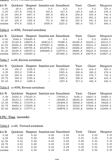
The number of comparisons has been plotted against the sortedness ratio on lists of length

64, 256, 1024 and 4096 and the sortedness ratio was varied between 0% and 25% and between

0% and 25% on a reverse ordered list. Results were gathered on reverse ordered lists as the

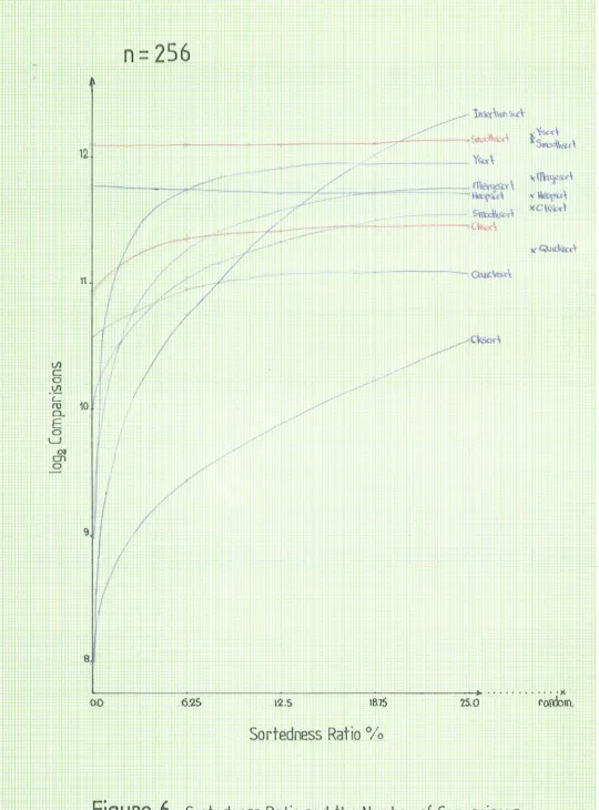
decision of a list being sorted when its elements form a non decreasing sequence is arbitrary. The number of comparisons were also plotted against lists with a completely random order

which highlighted some algorithms which had good performance on nearly sorted lists but bad

performance on lists in which the elements were in a random order. For the lists of length 4096 the CPU time was also plotted against the sortedness ratio. The CPU time was not considered

the main criterion for evaluation of the algorithm's efficiency as the time may depend on

machine features such as system overhead, disc accesses, time slicing etc, but the CPU time

should reflect the algorithms complexity and relationships of CPU time and the number of

comparisons should give similar curves when plotted against the sortedness ratio.

Each point on the graphs represent an average of 10 trials. Lines in red indicate lists with

reverse sortedness and have only been plotted when the forward and reverse sortedness differs significantly, as is the case with cksort and smoothsort. Appendix B contains a complete list of

the results for lists of size 64 and 4096.

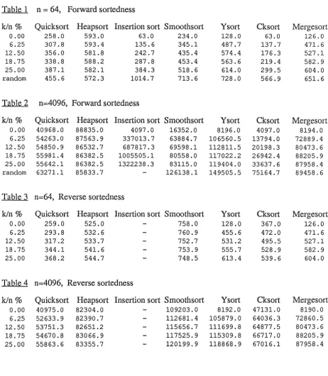
Linear insertion sort performed well on lists that were very close to being sorted, and for a

list of length 64 linear insertion sort was one of the better sorts compared. As the length of the

list increased the efficiency deteriorated compared with the other sorting algorithms tested. This

is mainly due to the average distance of elements from their final position, in the sorted list,

increasing as the length of the list increases.

Unfortunately insertion sort's efficiency on a reverse sorted list and lists that have sortedness

ratio in reverse represents the worst possible case and the algorithm deteriorates to its known complexity of O(n2). For this reason it was impractical to collect statistics when the list was

sorted or nearly sorted in reverse.

Ysort and natural mergesort were not the best sorting algorithms analysed but they have

several features that make them worth considering. Both sorting methods are symmetrical in that

they handle reverse sorted or nearly sorted lists in an ascending manner equally well, making

these two sorting methods more robust than some of the other methods analysed. This is an

important feature since in practice a list may be nearly sorted in reverse as frequently as it is

nearly sorted in an ascending manner and it makes sense to exploit this feature in a sorting

algorithm.

Both ysort and mergesort lose their O(n) efficiency characteristics quickly compared with the

sortedness ratio and the longer the list the faster the algorithms approached their worst case

complexities of O(n log n). For a list of size 4096 these algorithms were close to their worst

case complexities for a sortedness ratio of about 6%.

Smoothsort has a greater number of initial comparisons than all the other sorting methods

compared but it soon becomes more efficient when compared with other sorting methods such

as mergesort, heapsort and ysort. However, the performance of the algorithm does not support

Dijkstra's claim of a smooth transition from O(n) to O(n log n) complexity as the list becomes

unsorted. The worst case for smoothsort occurs on a reverse list which it is not capable of handling in O(n) time as the heap is built with its leaves at the left of the list and the roots of each

heap, which are the greatest elements of each heap, at the right of the list.

Cksort is the best sorting technique analysed. It had the smoothest transition from an O(n) complexity on a sorted list to an O(n log n) complexity on an unsorted list. For a list with

varying kin ratio in an ascending order cksort was unsurpassed. The descending sequences

proved a problem for cksort with both ysort and mergesort being more efficient initially and

while the list was close to sorted (kin ratio in the range 0% to 5%). The bad performance on

reverse lists is due to the design decision to extract elements from the initial list if they are

descending pairs. For a reverse list most of the elements will be descending pairs and will be

extracted and then sorted by quicksort resulting in an O(n log n) complexity.

The graph of the CPU time against the sortedness ratio, figure 9, confirms the complexity of

the algorithms, as the curves for most algorithms reflect the curves obtained for the number of

comparisons graphed against the sortedness ratio. Mergesort appears to be a more efficient

algorithm when its CPU time is drawn against other algorithms, but this is due to the recursive

nature of most of the algorithms and the iterative nature of the mergesort algorithm. Quicksort is

the most efficient, in terms of CPU time, when the list is totally unsorted.

C'OF!MAC. + r,

'r

,f

µ_ ,L ~

,~ t

+i,

J

~

H ,,_

-H µ

ff

Ill I II I I I

t

~

l

f

I I '

j '

'

:t

_,

-c

I t

l ~ I :.i-+

t

~ U) c 0 U) . c:::

ro 0. E 0 LJ 'Ol CTl 9

_g 7

,,

Iffll!T

.S f , ~

~

1'/1«~

"~so-\

·~~

S i ~

. ~r:,o<t

·~ ~rt

~Q.)\~

'---...µ...----1---+- - - + - - - , - - - ----... ... x

6.25 fQ\\ct011\

Sortedness

Ratio

0

/o

11

,

Figure 5.

Sortedness

Ratio and the Numbe

r

of Comparisons.

-:°'·•'..·.

··.·

:, .. .':.::.-~-:

'·-" ·.·

,

~~~~-:::~#2~...,....;~+-,+....,--~~===-'7'1"""-="==;:::;.;=:;:;::::;::::

·

_·,-ia;~<

~~y\

_\

- - - ~ - , S ~ ~ \

----~~,... ... ~·=

11

-"·-~-~~

cw

,c(

\

l<~1fS'r\

.... ·~ \ l(C\<.r.prt

~

---~---~---~---

.-+

...

.

....

x

6.'25 18.75 25.0

rorrurn

.

Sortedness

Ratio

0

/o

Figure 6.

Sortedness

Ratio

and

the Number of

Comparisons.

[image:30.597.11.551.35.764.2]

I

I

i

j.

l

i1L

1ll!1

11111 1A

1

1

111 I

"' 1· i111 _'

I I

(/)

c

0

(/)

L

ro

0..

E

0

LJ

~

_g

H

n=1024

6.25

. . _ _ - - - -- ~· . . . • l(

12 .5

,s.

75

1.':>.0 rol\dom

S

ortedness Ratio

0

_/o

I ,

F

igur

e

7.

Sortedness

Ratio

and

the Number of

Comparisons.

.-._··_.·-.·.· .·.-.·

[

I V)

c

' o

1.1)

!

-(_

ro

Cl. I

'E 0

LJ

C\l

en

_Q

I I

;1tl-vJ~.;,,<r

),(

l

ta:f'.P

'

~

x~t

.

...

.

.

..

.

.

..

,.

f'Ol)ODIT\

Sortedness Ratio

0

/o

U)

tJ

c

(D

u

aJ

~

aJ

.

_-+-

~

=>

n..

LJ

N

cr,

..9

.,..s\"X:<l\"6:icl

'<'(:-.cd

5~ 1

·~~('~

"'~"

~ H

.><C~t

·tJer~ X~_r'cOI'\

,0.1J1c\i.8:;r.\

.J(Q.\lt:\l,.<;Ofl

~C\<.'i!::.'1'\

\8.15

~ "'"rr'-~~c--- t - -~ ~ ~- - l - -~ - - ; - -- ----:-7'---:'--+-I '"?"?" .•..• ' ... )\ '

2s.o

ran~6m

Sortedness

Ratio

0

/o

9

Sortedness

Ratio

and

the

CPU

time.

:.::->::~:

. ~ . ·-·

',t~.::.;

r..-.,·,~ ..

3.7 Conclusions

From the graphs of the results it can be seen that if the structure of the list is unknown

quicksort remains the best internal sorting algorithm, since it out performs all other algorithms

when the list is unsorted. When the sortedness ratio of the list is greater than 5% quicksort is only outperformed by cksort, except for when the list is very short, when linear insertion so1t is

also more efficient. For very short lists linear insertion sort is the best algorithm to implement

due to its short simple code even though it may not be the most efficient in terms of the number

of comparisons. For lists that are known to be nearly sorted in an ascending manner cksort is

the best algorithm to implement, but the bad performance of this algorithm on lists that are

nearly sorted in reverse and on random lists make quicksort the more preferable algorithm under

these conditions.

Of the other algorithms compared, several of them, ysort and mergesort, handled lists that

were nearly sorted in reverse as efficiently as list that were nearly sorted in an ascending

manner, but the transition from O(n) to O(n log n) complexity was rapid making quicksort the

more preferable algorithm for all but very nearly sorted lists. Smoothsort was easily outperformed by cksort and in most cases quicksort as well. Smoothsort could not efficiently

sort lists with reverse sortedness and the algorithm is also the most complicated. For these

reasons it is not a suitable algorithm to implement under any situations.

The ideal algorithm should provide the best performance under all situations. Lists with

ascending and descending sortedness could be handled efficiently and there would be a smooth transition from O(n) to O(n log n) complexity as the list became more unsorted. The graphs

highlighted several deficiencies in each of the algorithms analysed and none of the algorithms

considered gave ideal performance under all conditions.

4.0 IMPROVEMENTS, MODIFICATIONS AND OTHER IDEAS

The results in the previous sections showed many of the deficiencies in the algorithms implemented and this motivated changes to the algorithms in the hope of decreasing the number

of comparisons required to sort a list. Attempts to modify the algorithms to cater for lists with

reverse sortedness and random order were made. In some cases simple changes resulted in

dramatic increases in performance and more elaborate changes resulted in a degradation of performance. Particular attention was paid to cksort as it had the best performance for lists with

an ascending sortedness ratio and had the potential to be the best all round algorithm analysed.

Where improvements in an algorithm's performance have occurred results have been graphed against the unoptimized version on lists of size 4096. Appendix B contains a complete list of the

results for the optimized versions for lists of length 64 and 4096.

4.1 Improvements to Y sort

Although ysort has good performance on sorted and nearly sorted lists (kin in the range 0%

to 5%), its performance deteriorates rapidly to its O(n log n) behaviour. The major reason for

this deterioration is the expense in finding the maximum and minimum values of the left and

right subfiles. If the subfiles are unsorted then most of the elements will require two

comparisons to determine if they are the new maximum or new minimum element.

Ysort's biggest improvement over quicksort is in determining whether or not the subfiles are

sorted and not by calculating the maximum and minimum values of the subfiles. A more

efficient algorithm could then determine whether the list is sorted by taking only one comparison

per element. Also, without any additional comparisons the maximum or minimum element of

each subfile could be determined.

The ysort algorithm was modified with the following code placed after a subfile had been

partitioned:

{ for the left subfile} max:= 1

fork:= (1 + 1) to j do

if A[max] <= A[k] then

max := k else

lsorted := false swap(A[max], A[j])

and a similar piece of code to determine the minimum element of the right subfile and whether

Lil

c

I l ₀

Lil L

ro

0..

E

0 LJ

(\1

0 ,

_g

I

I

'I

'1

1

I

++

15

14

r{

13' I. r

.o.o

Sortedness Ratio

0

/o

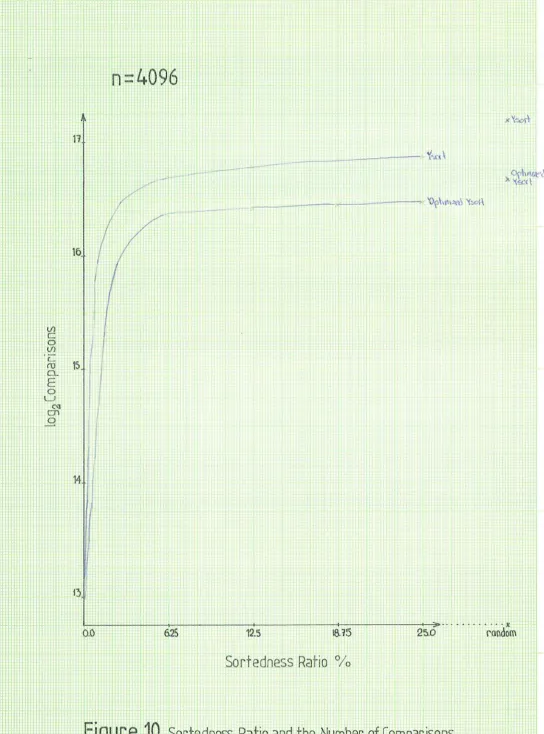
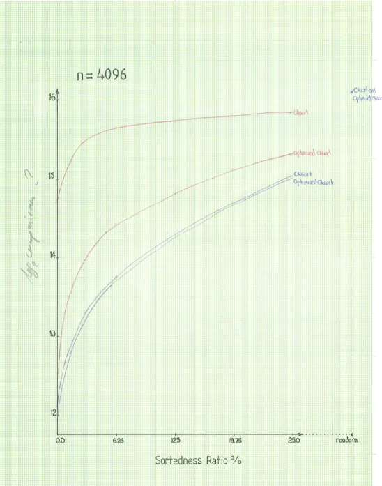
Figure 10.

Sortedness

Ratio

and

the Number of

Comparisons.

;.::·_···.

. .

f

'=<'.:

_{.·.· .·.}

..

[image:36.597.12.556.35.768.2]

the right subfile is sorted.

As can be seen, each element in each subfile now requires only 1 comparison to determine

whether the subfile is sorted and in addition the maximum value of the left subfile and the

minimum value of the right subfile are swapped into their correct place.

To sort the subfiles the last element of the left subfile and the first element of the right subfile

do not need to be considered as they are in their correct places. In the unoptimized algorithm

both the minimum and maximum element of each subfile are in their correct place after a file has

been partitioned.

The code to control sorting of the subfiles will then be as follows, where lsorted and rsorted

indicate whether the left and right subfiles are sorted and 1 and r are the leftmost and right most positions of the unsorted file:

if not lsorted then

sort the subfile A[l .. j-1]

if not rsorted then

sort the subfile A[i+l .. r]

The above changes resulted in significant improvements for lists of length 64, 256, 1024,

and 4096. Figure 10 shows the improvement for lists of length 4096 and Appendix B contains a

complete listing of all results for lists of length 64 and 4096. In all cases the biggest

improvement occurred when the lists was totally unsorted, but improvements occurred for all

degrees of sortedness.

4.2 hnproven1ents to Cksort

The algorithm for cksort is very effective and is the most efficient sorting algorithm analysed.

Its major deficiency is that it cannot process lists with reverse sortedness as efficiently as those

with forward sortedness. As can be seen from the graphs in the previous chapter, cksort is close

to its O(n log n) behaviour on lists with reverse sortedness.

An extension to the algorithm uses a third list C. Decreasing pairs are extracted from list A

and placed in list B as before, and increasing pairs are then extracted from list B and placed in

list C. This results in two sorted lists; A, which contains non decreasing elements, and B, which

contains non ascending elements. List C contains all the unordered pairs that were extracted

from list B and is sorted by quicksort if there are greater than 30 elements, and by linear

insertion sort otherwise. Finally all three list are merged into the original list A. Lists that are

sorted or nearly sorted in reverse will contain mostly decreasing pairs which remain in list B,

C,Or~MAC'I< C, lA H

I

I

t+ I

I

_I, ,, i

I

t

_#1

I

f

1f

I

l

+ I

' '

,

16

1

' '

_J

l'

f

I

'

I

: t

J: ;

tP

t, ' t

I

+

:t: t

'

'

'

\\.

1 I

15'

T

r

I V

1

t

+

I,,

' I

I

t

l

f

*

+I ·1

-.-,

14

i-

_f.

+

~' i: 1

r1 l~

I

t

_t3

I

I

~' -+

II

E

t

j

i

II

'

I

t

I

I I

12

I

n

+ ,,

I

1

:

-l-I I .0.

I

a

~

I

1

~

0, .6.25 12.'5 18.75

Sorte

_

do

_

ess Ratio

0

/o

I

f

:,

tt;

if

I, I I

1,J

11lt

II

' 1i

I

1:f:

f

~

I

J

CL

Fig

Ure

11.

Sortedness

Ratio

and

the Number of

Comparisons.

'

;,1C~O!\\

~h,,1~(1-'.t>rl

[:,):: 1·----,

I J..

[image:38.595.12.561.32.730.2]

resulting in a small number of unordered pairs in list C.

A further improvement results from partitioning until the subfiles are smaller than some

_ critical value and using linear insertion sort to complete the sorting on the partitioned subfiles.

The threshold value at which to stop partioning was selected as 10 [3]. This is a reasonably

simple improvement to make since the algorithm for linear insertion sort is contained within the

algorithm for cksort.

As can be seen from figure 5 to figure 9, cksort performed badly when the list was unsorted

and quicksort easily outperforms it in these situations. This is a result of a bad choice of

partition element. The ideal partition element is close to the median element of the the list being

sorted. Choosing the middle element as the partition element can result, and frequently does, in an element that is typically small or large compared with the other elements of the list being

sorted. This is because the unsorted list, list C in the improved algorithm, consists of pairs of

increasing elements. By choosing the mean of the two middle elements, a value that better

approximated the median was obtained resulting in fewer partition steps and therefore fewer

comparisons. For a random list of size 4096 this one simple modification resulted in almost a

10% reduction in the number of comparisons. The optimized algorithm is as follows.

list A list B list C

- the unsorted array

- contains the descending sequences. - contains the unordered pairs

Extract all decreasing pairs from list A (as before) and place in list B. Array A now contains a sorted non decreasing list.

Extract all increasing pairs from list Band place in list C. Array B now contains a sorted non ascending list.

if number of elements in list C is less than 30 then Sort list C by insertion sort.

else

Sort list C by quicksort, using a cutoff and insertion sort,

the partition element is the mean of the two middle elements.

Merge lists A, Band C into A.

The major modification to cater for reverse lists resulted in an O(n) complexity when the list

was sorted in reverse and a slight degradation in efficiency for lists with ascending sortedness. Both of the other two improvements resulted in an increase in efficiency for lists with both

forward and reverse sortedness, see figure 11. The biggest increase in efficiency as a result of

using a cutoff occurs when the list is unsorted as then a large portion of the original list will be

present in list C and require sorting by quicksort.

4.3 Alterations to Smoothsort

The sophisticated data structure of smoothsort makes it difficult to change the structure of the

program and almost impossible to improve the algorithm to cater for lists that are nearly sorted

in reverse. One of the simplest changes to the algorithm is to alter the branching factor of the

heaps. Previous results were obtained by using a binary heap. By using a ternary heap it was

hoped that the number of comparisons needed to sort a list would be reduced.

For a list of size n the upper bound for the number of binary heaps in a forest of complete

heaps is,

N2

=

r

log2n

l,

and the upper bound for the number of ternary heaps is,

N3

=

r

1.2618 log2n + 0.2618

l,

(see Appendix C). Experiments performed on lists of size 1 to 1000 showed that there was

typically a greater number of ternary heaps than binary heaps.

Sorting using a single ternary heap has been shown to have a better performance than a

single binary heap [7] due to fewer comparisons being required to sift an element to its correct

place within the heap. Results on lists of size 64, 256, 1024 and 4096 showed that smoothsort

was inferior in just about all cases and this can be attributed to the greater number of average

heaps required. For an unsorted list in the second pass of smoothsort a greater number of heaps

results in a greater number of swaps, and therefore comparisons, to move an element to its correct heap and this overcomes the advantage of fewer comparisons in sifting an element to its

correct place within a heap when using a ternary heap. For lists of length 4096, with the

sortedness ratio varied in an ascending manner the number of comparisons to sort a list are as follows:

kin% binaiy heaps ternary heaps

0.00 16344.0 16334.0

6.25 60098.5 75755.4

12.50 69598.1 89833.7

18.75 80558.0 104173.2

25.00 83115.0 105701.5

The number of comparisons for lists of length 64, 256 and 1024 gave similar results with a

forest of binary heaps having a better performance in almost all cases. A forest of ternary heaps

gave almost the same number of comparisons when the list was completely sorted. However as

the list became unsorted a forest of binary heaps always had a better performance. For a

sortedness ratio of 25% and a list of length 64 a forest of binary heaps had 12% fewer comparisons and for lists of length 256, 1024 and 4096 a forest of binary heaps had at least

20% fewer comparisons.

4.4 Alterations to Linear Insertion Sort

Although linear insertion sort has a very bad worst case performance it gives the best results,

along with cksort, when the list is sorted in an ascending manner. Modifications to insertion sort

to improve its performance when the list is not sorted are worthy, since the code is short and simple and the algorithm is frequently implemented by itself, and as a hybrid algorithm.

The biggest disadvantage with linear insertion sort is a result of the O(n2) comparisons it performs when the list is unsorted. To overcome this problem and to preserve the algorithm's

best case performance the algorithm was modified.

During the sorting of a list of n elements the following situation exists:

1 2 3 k n

I I I I· ....

_{I I}

_{I I}

sorted list

l

unsorted list element to sod

The implemented algorithm performs a linear search from right to left to locate the correct

position for the unsorted element. However, the list it searches is in fact sorted and an improvement would be to use a binary search to locate the position for the unsorted element.

This would eliminate insertion sort's best case performance since it would not necessarily

compare the unsorted element with the element immediately to the left. To overcome this the

sorted list is first searched using a divergent binary search to isolate the region for the new

element and then using a conventional binary search to isolate the correct position for the

element. For example, consider the list above being sorted by this algorithm when the next

element to be sorted is at position k. The element is compared with elements at positions k-1,

k-3, k-7, k-15, ... In this way the correct region for the element can be located in O(log2 k)

comparisons. The actual position for the element is then isolated using a conventional binary

search on the region determined and will take at most O(log2 k/2) comparisons. In this way the

conect position for an element can be located with

O(log2k) + O(log2k/2)

=

O(log2k)

s; _O(log2n),

comparisons and yet only one comparison is required if the list is sorted. This may seem an

ideal solution to the problem but once a position is located there may be O(n) swaps to move the unsorted element into position giving the algorithm a worst case time complexity of O(n2) as

before.

In an attempt to overcome the possible O(n2) complexity when sorting a list the following

data structure that incorporated pointers was used:

linked lists in sorted

order

sorted order

1 2 3 4 5 n

To locate the correct position for an element within the so1ied list the array is searched using

first a divergent binary search and the a convergent binary search as before. For each

comparison the element at the head of the list is compared with the unsorted element. O(n log n) comparisons are required to locate the correct linked list to search. The correct position within

the list is then located by using a linear search and the unsorted element is inserted into the list

without causing any swaps.

Unfortunately this algorithm had an inferior performance compared to straight linear insertion

sort. The best case performance was preserved for completely sorted lists, but as the sortedness

ratio increased straight linear insertion sort easily outperformed the new algorithm. With a

sortedness ratio of 6.25% and a list of length 64 the new algorithm had more then 3 times as

many comparisons and for higher sortedness ratio or with longer length lists there was even

more comparisons required for the new algorithm.

The problem with this algorithm can be seen when sorting the list,

10 1 2 3 4 5 6 7 8 9,

which has a sortedness ratio of 0.1 and is therefore nearly sorted. The algorithm inserts each

- element at the head of the first linked list and the advantage of using binary search to locate the correct position has been lost, since the current sorted list consists of only one linked list.

Suppose the first 4 elements have been sorted then the situation is as follows.

1 2 3 4

To insert the next element, 4, the complete chain has to be traversed to locate the correct

position, and the algorithm is equivalent to straight linear insertion sort with respect to the number of comparisons. Also the new algorithm had a considerable slower execution time due

to pointer manipulation.

5.0 CONCLUSIONS

Of all the algorithms compared the optimized cksort had the best performance in all cases,

except for when the list was very unsorted, and then quicksort only outperformed cksort by a

linear factor. However quicksort is a considerably easier algorithm to implement and if the

structure of the list is unknown, or if it is known that the list is most likely to be totally unsorted

then quicksort is probably the more preferable algorithm to implement.

As mentioned previously, cksort, and the other algorithms, have been analysed using a

measure of sortedness that cksort exploits efficiently, whereas in practice the sortedness ratio

may not best capture the sortedness properties of a nearly sorted list. For example, consider the

list,

n/2 + 1, n/2 + 2, ... , n, n/2, n/2 - 1, ... 1,

which consists of an ascending and descending sequence and has a sortedness ratio of 1/2.

Cksort would require all the elements to be sorted by quicksort and the optimized algorithm

would require n-2 of the elements to be sorted by quicksort, in both cases the algorithms would

have a complexity of O(n log n) on this list. On the the other hand, sorting the list by natural

mergesort would require only two passes and therefore have a complexity of O(n) on a list with

this structure.

The development of faster algorithms for nearly sorted lists requires measures of sortedness

that better capture the properties of a list that allow O(n) time sorting. These measures should

also return appropriate values for nearly sorted lists that occur in practice and not be confined to

a theoretical definition of a nearly sorted list.