1
Selenium isotopes as a biogeochemical proxy in deep time
Eva E. Stüeken
Department of Earth & Space Sciences and Astrobiology Program University of Washington
Seattle, WA 98195-1310, USA
Department of Earth Sciences University of California Riverside, CA 92521, USA
Department of Earth & Environmental Sciences University of St. Andrews
St. Andrews, KY169AL, UK
INTRODUCTION AND OVERVIEW
Most research on selenium isotopes over the last decade has focused on either one of two avenues in biology and low-temperature geochemistry. Environmental and biological studies of modern systems are primarily concerned with monitoring and controlling the mobility of selenium in terrestrial settings. Selenium is an essential micro-nutrient for many organisms, including humans, but it becomes toxic at high concentrations (Zwolak and Zaporowska 2012). Significant efforts are therefore invested into evaluating the toxicity, mobility and bioavailability of selenium in soils, rivers and agricultural products. Geochemical studies of ancient sedimentary rocks, on the other hand, make use of the redox active nature of selenium to reconstruct atmospheric and marine oxygenation over various spatial and temporal scales (e.g. Rouxel et al. 2004; Mitchell et al. 2012; Layton-Matthews et al. 2013; Pogge von Strandmann et al. 2015; Stüeken et al. 2015a; Stüeken et al. 2015d; Stüeken et al. 2015c; Mitchell et al. 2016). This review will focus on the latter aspect, noting that extensive reviews of environmental problems are provided elsewhere (e.g. Hamilton 2004; Banuelos et al. 2013; Plant et al. 2014)
Selenium (atomic number 34, average mass 78.971 amu, Table 1) is classified as either a metalloid or a non-metal, depending on the allotrope of elemental Se(0) (Fernandez-Marinez and Charlet 2009). It belongs to the chalcophile elements that have a high affinity for sulfur and are enriched in sulfidic ore deposits (Goldschmidt and Strock 1935; Goldschmidt 1937). It is part of the same group as sulfur in the periodic table and shares a number of chemical properties. Like sulfur, selenium has six electrons in its outer shell, two in the 4s subshell and four in the 4p subshell, but unlike sulfur, it possess a full 3d subshell that lies interior to the outer electrons and provides relatively poor shielding from the nucleus (Greenwood 1984). As a result, the six outer electrons feel a relatively stronger attraction, which leads to a higher energy demand for selenium oxidation compared to sulfur.
2
minerals or organic compounds. While S(-II) is oxidized to a +VI state at relatively low redox potential, Se(-II) first goes to the thermodynamically stable forms Se(0) and Se(IV) during oxidation; its fully oxidized form (Se(VI)) is only stable at high Eh, similar to nitrate (N(V) in NO3-) (Fig. 1). Elemental Se(0) is a solid
phase that is formed by either incomplete reduction or incomplete oxidation and thermodynamically stable over a wide Eh-pH range (Fig. 1). It is found in sediments and soils (Martens and Suarez 1997; Herbel et al. 2002; Kulp and Pratt 2004; Clark and Johnson 2010; Fan et al. 2011), as well as in the colloidal fraction of rivers (Zhang et al. 2004; Doblin et al. 2006). Se(IV) and Se(VI) form oxyanions (selenite, SeO32-,
hydroselenite or biselenite, HSeO3-, and selenate, SeO42-, respectively) that are highly soluble (Seby et al.
2001). They are the major forms of selenium in the modern deep ocean and in river waters (Conde and Alaejos 1997; Cutter and Cutter 2001). Se(IV) has a relatively higher affinity than Se(VI) for adsorption onto ferromanganese oxides, clay particles and organics, in particular at low pH (e.g. Bar-Yosef and Meek 1987; Balistrieri and Chao 1990; Rovira et al. 2008; Mitchell et al. 2013). Furthermore, trace amounts of both Se(IV) and Se(VI) can be incorporated into carbonate minerals by substitution for CO3- (Reeder et al.
1994; Aurelio et al. 2010). Selenium associated with sulfate evaporites appears to be minor (Hagiwara 2000). The major forms of selenium in siliciclastic sediments are organic- and pyrite-bound Se(-II) (Kulp and Pratt 2004; Fan et al. 2011; Schilling et al. 2014a; Stüeken et al. 2015c). Atmospheric selenium gases primarily comprise methylated selenides that are produced by a variety of bacteria, plants, fungi and algae (e.g. Zieve and Peterson 1984; Amouroux et al. 2001; Chasteen and Bentley 2003; Schilling et al. 2011b); however, they have a short lifetime of only a few hours because they are rapidly oxidized in the modern oxic atmosphere (Wen and Carignan 2007). Volcanic processes may produce H2Se gas, but this rapidly
oxidizes to Se(0) today (Suzuoki 1965). Similarly, gaseous SeO2 condenses rapidly below 315°C and is thus
not nearly as volatile as SO2, the equivalent compound in the sulfur cycle (Wen and Carignan 2007; Floor
and Román-Ross 2012). Hence >80% of volcanic selenium emissions are in particulate form (Mosher and Duce 1987).
Overall, selenium has a complex biogeochemical cycle and undergoes numerous transformations between weathering and burial. Its properties suggest that fluxes, reservoirs and speciation have changed multiple times over the course of Earth’s history with the evolution of the atmosphere, oceans and life. Selenium isotopes are a newly emerging proxy for reconstructing the evolution of the global selenium cycle.
NOMENCLATURE, REFERENCE MATERIALS AND ANALYTICAL TECHNIQUES
Some of the first studies of selenium isotopes were conducted by gas-source mass spectrometry where selenium was introduced via fluorination to SeF6 gas, following similar protocols as for sulfur
isotope measurements (Krouse and Thode 1962; Rees and Thode 1966). The prime limitation of this method was the high selenium demand of > 10g. Later studies used thermal ionization mass spectrometry (TIMS) which had at least tenfold higher sensitivity (Wachsmann and Heumann 1992; Johnson et al. 1999; Herbel et al. 2000). Traditionally, TIMS operates with cations, but Se+ production is
energetically unfavorable. To circumvent this problem, a negative ion method was developed for TIMS analyses. Nowadays, selenium isotopes are most commonly analyzed by multi-collector inductively-coupled plasma mass spectrometry (MC-ICP-MS) (Rouxel et al. 2002; Elwaer and Hintelmann 2008b; Zhu et al. 2008; Schilling and Wilcke 2011; Mitchell et al. 2012; Stüeken et al. 2013; Pogge von Strandmann et al. 2014). The sample is introduced via cold-vapor hydride-generation (HG), which produces gaseous H2Se
3
analyses of as little as 10ng Se under optimal conditions (Rouxel et al. 2002). MC-ICP-MS allows monitoring all selenium isotopes as well as surrounding masses that may be needed to correct for isobaric interferences.
Interfering elements include residual germanium and arsenic derived from the sample matrix, as well as compounds generated from the argon carrier gas and the hydrochloric acid that contains the dissolved H2SeO3 (Table 1). Interferences are most severe for m/z = 80, where argon dimers are most
abundant. This problem can be ameliorated with a collision cell that reduces dimer production (Rouxel et al. 2002; Layton-Matthews et al. 2006). Nevertheless, results for 80Se are usually not reported. Similarly
problematic is 74Se, which has the lowest abundance and is easily masked by traces of 74Ge (Table 1).
Measurements of 76Se can be compromised by 75AsH in arsenic-rich samples, requiring accurate correction
protocols (e.g. Stüeken et al. 2013). In rare cases, 75AsH
2 becomes significant and interferes with 77Se
(Stüeken et al. 2015a). Data for 78Se and 82Se are comparatively clean.
Two different methods are in use to correct for instrumental mass bias (isotopic fractionation during the transmission of Se ions from the source to the detector) and drift (temporal change of the instrumental mass bias due to slow changes in temperature, vacuum quality, etc.). These methods include double-spiking (e.g. Johnson et al. 1999; Zhu et al. 2008; Schilling and Wilcke 2011; Mitchell et al. 2012; Pogge von Strandmann et al. 2014) and standard-sample bracketing (SSB, e.g. Rouxel et al. 2002; Layton-Matthews et al. 2006; Stüeken et al. 2013). Double-spiking means that at an early stage during sample preparation the sample is spiked with a solution that is artificially enriched in two selenium isotopes. The major advantage of this technique is that isotopic fractionations imparted during sample preparation can be monitored and corrected. SSB, on the other hand, requires close to 100 % yields because fractionations during sample preparations cannot be tracked independently. Double-spiking therefore generally leads to higher precision (2≈ 0.1-0.3 ‰than SSB (2≈ 0.2-0.4 ‰) for geological samples. A disadvantage of double spiking is that it requires measurements of at least four isotopes and is thus more prone to isobaric interferences (Table 1). With SSB, accurate isotopic measurements can be made with only the two most interference-free isotopes. Furthermore, if the isotopes enriched in the double spike are affected by any mass independent fractionation, then a second, unspiked analysis is required. Lastly, the quality of interference corrections cannot be monitored with three-isotope diagrams when a double-spike is used. SSB leaves the option of detecting mass-independent fractionation and isobaric interferences, because multiple natural isotope ratios can be monitored. A detailed description of how to implement a selenium double-spike is given by Johnson & Bullen (2004a).
4
(TCF) that can be prepared in the laboratory from commercial cotton balls, soaked in a mixture of acetic acid glacial, acetic acid anhydride, mercaptoacetic acid and sulfuric acid (Yu et al. 2002). Some recent studies replaced cotton balls with cellulose powder (Elwaer and Hintelmann 2008a). TCF removes most matrix elements, but it cannot completely remove germanium and arsenic, which cause important isobaric interferences in the mass spectrometer (Table 1, Stüeken et al. 2013). Germanium can be removed effectively by hydride generation (Clark and Johnson 2010) or by treating the sample with aqua regia (Stüeken et al. 2013).
Selenium isotope data are typically normalized to NIST SRM 3149, which is distributed as a solution. Some older reference standards, in particular MERCK, have been calibrated relative to NIST SRM 3149 by Carignan & Wen (2007), where δ82/78Se
NIST3149 ≈ δ82/78SeMERCK + 1.03‰. Variations in analytical
methods dictate different choices of the isotopic ratio that is used to report the data. Some studies report data in terms of 80Se/76Se (Johnson et al. 1999; Herbel et al. 2000; Herbel et al. 2002; Clark and Johnson
2010), but most recent work uses either 82Se/78Se (Stüeken et al. 2013) or 82Se/76Se (Rouxel et al. 2004;
Mitchell et al. 2012; Layton-Matthews et al. 2013; Pogge von Strandmann et al. 2014; Schilling et al. 2015).
82Se/78Se has the major advantage that isobaric interferences are relatively minor for both isotopes
(Stüeken et al. 2013), particularly in sediments with high arsenic concentrations (Stüeken et al. 2015a, unpublished data), where m/z = 76 can be compromised. As long as mass-independent fractionation is absent (Stüeken et al. 2015d), 82Se/78Se can be converted to 82Se/76Se by multiplication with a factor of
1.539 for equilibrium fractionations and 1.519 for kinetic fractionations, assuming atomic rather than molecular masses (Young et al. 2002). The difference between the two factors is less than 0.1‰ for fractionations up to 5‰ and hence within analytical error in most cases. Isotopic data are conventionally presented in delta notation in units of permil (Equ. 1):
82/78Se [‰] = ((82Se/78Se)
sample/(82Se/78Se)SRM3149 - 1) ∙ 1000 (1)
To determine analytical accuracy, recent studies reported measurements of the USGS rock standard SGR-1, which is an Eocene oil shale with 3.51 ± 0.26 ppm selenium (Savard et al. 2009). Results for 82/78Se range from -0.13 ‰ to +0.40 ‰ with a mean between seven studies of +0.14 ± 0.19‰ (1),
after conversion to the NIST SRM 3149 scale (Rouxel et al. 2002; Layton-Matthews et al. 2006; Schilling et al. 2011a; Mitchell et al. 2012; Pogge von Strandmann et al. 2014; Schilling et al. 2014a; Stüeken et al. 2015d). Other less common reference materials that have been analyzed for selenium isotopes are listed by Rouxel et al. (2002) and Layton-Matthews et al. (2006).
ELEMENTAL AND ISOTOPIC ABUNDANCES IN MAJOR RESERVOIRS
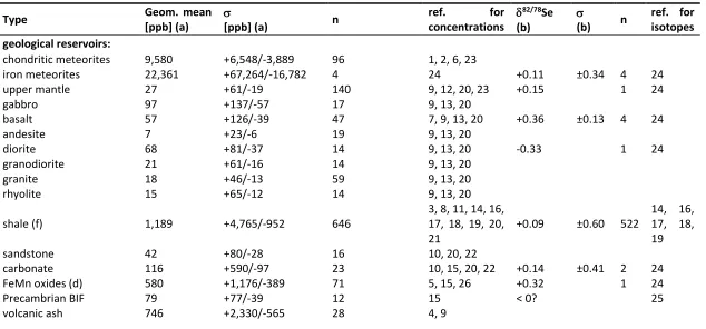
Selenium concentrations have been measured in a variety of natural substrates over the past century (e.g. Goldschmidt and Strock 1935), but accurate isotopic analyses have only been possible since the late 1990s with the establishment of TIMS and associated advances in analytical sensitivity. Our knowledge of isotopic partitioning in natural systems is therefore still severely limited. In compiling information about major geological reservoirs, selenium concentrations and isotopic compositions almost always had to be taken from different sources (Table 2). Selenium concentrations often spread over an order of magnitude within each reservoir and are therefore expressed as geometric means.
5
The isotopic compositions in extraterrestrial materials and igneous rocks on Earth have not yet been studied systematically. Iron meteorites (~23 ppm, +0.11 ±0.34 ‰, Rouxel et al. 2002) and chondrites (~9.6 ppm, Table 2), the building blocks of the terrestrial planets, are relatively selenium-rich compared to geological reservoirs on Earth (mostly < 1 ppm, Table 2), suggesting that (a) most of Earth’s selenium partitioned into the core (Rose-Weston et al. 2009; König et al. 2012), and (b) impacts may have enriched the crust with selenium after core formation (Rose-Weston et al. 2009; Wang and Becker 2013).
The concentration of selenium in Earth’s upper crust has previously been calculated from the concentration of sulfur and an assumed sulfur/selenium ratio of 6000 (Goldschmidt and Strock 1935), yielding a value of 50 ppb (Turekian and Wedepohl 1961; Taylor and McLennan 1995). Wedepohl (1995) used a different approach whereby the concentrations of individual reservoirs were weighted by to their relative mass. According to this scheme, upper crust is composed of 14% sediment (44% shale, 20.9% sandstone and greywacke, 20.3% volcanic ash, 14.6% carbonate), 50% felsic intrusives (50% granite, 40% granodiorite, 10% tonalite), 6% gabbro, and 30% metamorphic rocks (64% gneiss, 15.4% schist, 17.8% amphibolite, 2.6% marble). Using concentration data available at the time, Wedepohl calculated an average concentration of 120 ppb. Adopting the same recipe and combining it with updated estimates of selenium concentrations and their standard deviations in the various reservoirs (Table 2), the new estimate of average upper crust presented here is 59 (+137/-41) ppb. An alternative recipe by Condie (1993), according to which upper Phanerozoic crust is composed of 25% tonalite-trondjamite-granodiorite (TTG), 11% granite, 16% felsic volcanics, 12% basalt, 12% andesite and 24% greywacke, leads to a selenium concentration of 34 (+26/-15) ppb. In this calculation, greywacke was approximated with 50% shale and 50% sandstone, and TTG replaced with granodiorite. The average isotopic composition is less well constrained, because the sedimentary record may be slightly biased (Stüeken et al. 2015d, discussed below) and very few igneous rocks and no high-grade metamorphic rocks have been analyzed to date. Taking the mean of basalts (+0.36 ± 0.13‰) and diorite (-0.33‰) gives a value of +0.01 ± 0.49‰ (Table 2), which may be our current best estimate for bulk crust. This number is consistent with a mass balance of marine sediments presented below.
Reservoirs at the Earth’s surface
Selenium is mobilized from the crust by oxidative weathering and transformation into oxyanions. These are bioavailable to organisms and can be subject to re-reduction in the presence of organic or inorganic electron donors (e.g. Stolz et al. 2006; Fernandez-Marinez and Charlet 2009; Schilling et al. 2015; Winkel et al. 2015). The interplay of oxidation and reduction controls the abundance and speciation of selenium in soils. To first order, selenium in soil is determined by bedrock composition (e.g. Malisa 2001). Unusually high concentrations (up to 26,000 ppm) and large isotopic fractionations of >20‰ were reported from a weathering profile through selenium-rich pyritic black shale (Zhu et al. 2014). A slightly smaller isotopic range (up to 7‰) was described from another seleniferous soil with up to 4 ppm selenium (Schilling et al. 2015). On the other hand, soils with concentrations closer to average crust (up to 0.5 ppm) showed a much smaller range of fractionations (±0.25‰, Schilling et al. 2011a). An important factor influencing the isotopic behavior of selenium in soils appears to be the abundance of organic matter and other reductants that re-reduce selenium oxyanions deeper in the soil profile (Zhu et al. 2014; Schilling et al. 2015). This and other processes further affect selenium uptake into plants (Winkel et al. 2015).
6
+2.5‰ for Se(VI), Clark and Johnson 2010), it is uncertain what the isotopic composition of modern rivers is. The isotopic difference between Se(VI) and Se(IV) found by Clark & Johnson (2010) suggest that at this particular site some Se(VI) is subject to reduction to Se(IV). Hence these data may be affected by local biogeochemical processes. As discussed below, mass balance of marine sediments suggests that the isotopic composition of the global average river flux is close to average continental crust (~ 0 ± 0.5‰, Table 2).
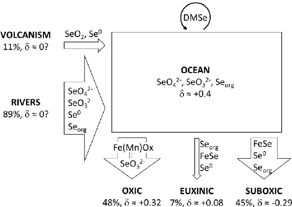
Selenium concentrations in seawater are consistently low (1-2 nM, Table 2). In the modern oxic ocean, Se(IV) and Se(VI) are the most abundant selenium species (Fig. 2). They both show a typical nutrient behavior with depletion in the photic zone and constant concentrations at depth, which reflects assimilation into biomass followed by remineralization of sinking organic matter (Cutter and Cutter 2001). Se(IV), which is produced by oxidation of organics, is thermodynamically unstable in modern oxic seawater, but the oxidation to Se(VI) is kinetically slow (Cutter and Bruland 1984). Therefore, Se(IV) accumulates in the deep ocean. In the photic zone, organic selenide dominates (Cutter and Bruland 1984; Cutter and Cutter 2001). Under anoxic conditions, as in the modern Black Sea, remineralization of organics is limited, such that organic selenide persists throughout the water column, while oxyanions are suppressed (Cutter 1982; 1992). The isotopic composition of dissolved selenium in seawater has so far not been measured directly, because the concentrations are too small. However, data from ferromanganese nodules and marine algae that assimilate selenium with minimal fractionation in the photic zone may provide a lower limit of +0.3‰ (Rouxel et al. 2002; Mitchell et al. 2012). Taking into account potential fractionations during adsorption and assimilation (discussed below), it is probably no higher than +0.9‰ and closer to +0.4‰. Because both Se(VI) and Se(IV) are produced by oxidation of organic matter, which imparts no detectable fractionation (Johnson et al. 1999), their isotopic composition is probably the same today. As noted below, this may not have been the case in the Precambrian when some Se(IV) may have been produced by Se(VI) reduction in the water column.
The nutrient-style behavior is a reflection of the strong accumulation of selenium in marine
biomass. For illustration, sulfate (~23 mM in seawater, Henderson and Henderson 2009) is about seven
orders of magnitude more abundant in the modern ocean than Se(IV) and Se(VI) combined, but only four orders of magnitude more abundant in aquatic microbial biomass (Fagerbakke et al. 1996; Mitchell et al. 2012). Settling of organic matter to the seafloor is therefore a major pathway of selenium export from the ocean into sediments (Fig. 2), especially in anoxic water columns. Furthermore, selenium assimilation can lead to the production of methylated selenide gases that partly escape into the atmosphere.
Dimethyl selenide and dimethyl diselenide are the major atmospheric selenium gases (Mosher and Duce 1987; Wen and Carignan 2007), and marine organisms are their main producers, which has led to the idea that this may constitute a transport mechanism of selenium from the ocean to continents (Amouroux et al. 2001). Methylated selenides have a short atmospheric residence time of only a few hours (Wen and Carignan 2007), which probably makes them insignificant on geological timescales. They are rapidly oxidized and converted into particulates, joining the pool of atmospheric particulates that are produced by volcanism and other sources (Mosher and Duce 1987; Wen and Carignan 2007). Mosher & Duce (1987) estimated that nowadays 40% of all selenium emissions into the atmosphere are of anthropogenic origin. The isotopic composition of gaseous selenium has not yet been determined, but methylated selenides are probably isotopically light, given the negative fractionation observed during volatilization experiments (discussed below, Schilling et al. 2011b; 2013).
7
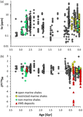
2015a; Stüeken et al. 2015d; Stüeken et al. 2015c; Mitchell et al. 2016). The bulk average isotopic composition of all published post-Sturtian (< 700 Myr) marine shale data is -0.14 ± 0.61‰ (1, n = 356(Johnson and Bullen 2004b; Shore 2010; Mitchell et al. 2012; Wen et al. 2014; Pogge von Strandmann et al. 2015; Stüeken et al. 2015d; Stüeken et al. 2015c). For the earlier Precambrian, it is +0.40 ± 0.51‰ (1, n = 247) (Pogge von Strandmann et al. 2015; Stüeken et al. 2015a; Stüeken et al. 2015d). As noted below, this difference may be a reflection of changing redox conditions during weathering and transport to the ocean. Sequential extraction studies of a few Phanerozoic shales showed that, in general, most selenium is contained in organic matter, but significant fractions are pyrite-hosted or present as adsorbed Se(IV) or elemental Se(0) (Martens and Suarez 1997; Kulp and Pratt 2004; Clark and Johnson 2010; Fan et al. 2011; Schilling et al. 2014a; Stüeken et al. 2015c). Where isotopic measurements were conducted, the adsorbed Se(IV) fraction often tended to be isotopically lighter than recalcitrant organics by around 1‰, possibly reflecting partial Se(VI) reduction under diagenetic conditions (Clark and Johnson 2010; Schilling et al. 2014a; Stüeken et al. 2015c). Elemental Se(0) was variable (Clark and Johnson 2010), and pyrite-bound selenide was isotopically light (Stüeken et al. 2015c).
Modern marine ferromanganese oxides (> 0.5 ppm, Table 2) constitute the second-most selenium-rich reservoir in the ocean after black shales. So far, only one isotopic measurement has been made, producing a value of +0.32‰ (Rouxel et al. 2002). Ferromanganese crusts and nodules are common in deep-sea sediments today. They can also be found as minute particles mixed with pelagic clays. Se(IV) in particular has a high sorption affinity for oxide minerals (e.g. Bar-Yosef and Meek 1987; Balistrieri and Chao 1990; Rovira et al. 2008; Mitchell et al. 2013). This mechanism may thus represent another important exit channel of selenium from the ocean (Fig. 2). Precambrian banded iron formations (BIF) contain comparatively less selenium (< 0.1 ppm, Table 2) and appear to be isotopically light (Schilling et al. 2014b), suggesting a different Se(IV) source (discussed below).
SELENIUM IN BIOLOGY
Organisms can make use of selenium in three different ways: (a) assimilatory reduction, or in short assimilation, which results in incorporation of selenium into proteins, (b) volatilization by conversion of selenium oxyanions into methylated selenides, and (c) dissimilatory reduction for metabolic energy gain or detoxification. Extensive reviews of these processes are provided elsewhere (Birringer et al. 2002; Boeck et al. 2006; Stolz et al. 2006; Gladyshev 2012). The following paragraph will highlight aspects that are relevant for geobiological studies.
(a) Assimilation: Some but not all organisms have an absolute requirement for selenium as a micro-nutrient (Stadtman 1974). These include vertebrates, protozoa, algae and several groups of prokaryotes (Birringer et al. 2002; Lobanov et al. 2009). Higher plants and fungi do not seem to have any selenium dependence, even though they can contribute to selenium methylation (discussed below). Selenium is used in its reduced form selenide, most commonly as part of the amino acid selenocysteine, sometimes called the 21st amino acid. It is structurally identical to cysteine, with a selenium atom in the place of
8
Steinbrenner and Sies 2009), may not have been significant until the 1st or 2nd Proterozoic rise of
atmospheric oxygen.
(b) Methylation and volatilization: Methylated selenium compounds primarily include dimethyl selenide and dimethyl diselenide and are produced by a number of bacteria, fungi, algae and plants in both aquatic and terrestrial environments (Chau et al. 1976; Chasteen and Bentley 2003). The evolutionary history of selenium methylation is unclear, but given that eukaryotic organisms are among the main producers of methylated selenides, this process may have gained importance in the late Neoproterozoic when eukaryotes became ecologically dominant (Knoll et al. 2006).
(c) Dissimilatory reduction: A variety of organisms, including Bacteria and Archaea, are capable of reducing selenium oxyanions to Se(0) in exothermic reactions that are sometimes used as sources of metabolic energy (Stolz et al. 2006). Se(VI) and Se(IV) reduction occur at higher Eh than sulfate reduction, i.e. under suboxic conditions. Se(VI) reduction is concurrent with denitrification (Fig 1., cf. Oremland et al. 1990). In fact, the selenate reductase enzyme appears to be phylogenetically related to nitrate reductase (Saltikov and Newman 2003; Watts et al. 2005). Some organisms that do not possess selenate reductase are able to reduce Se(VI) with nitrate reductases (Sabaty et al. 2001). Se(IV) reduction can be carried out by nitrite reductase (DeMoll-Decker and Macy 1993; Basaglia et al. 2007), but may in some cases also have multiple dedicated enzymes (Kessi 2006; Pierru et al. 2006). A specific selenite reductase has, however, not yet been isolated. Some sulfate-reducing bacteria are capable of Se(VI) reduction (Zehr and Oremland 1987), but it is unclear if this reaction is relevant in nature, if Se(VI) is removed at high Eh before sulfate-reducers become environmentally significant. Microbes that reduce selenium oxyanions in dissimilatory reactions usually excrete nanospheres of Se(0) (Stolz et al. 2006). Reduction of Se(0) to Se(-II) has also been described (Herbel et al. 2003), but the enzymatic pathways are still unknown.
ISOTOPIC FRACTIONATION PATHWAYS
Studies of isotopic fractionations have largely focused on low-temperature processes with particular emphasis on redox reactions. As is the case for carbon, sulfur and nitrogen isotopes, kinetic fractionations are likely dominating the selenium biogeochemical cycle and will be the focus of this review. Equilibrium processes can theoretically lead to large fractionations (Li and Liu 2011), but they are probably insignificant under most natural conditions, where various selenium species often coexist in disequilibrium (e.g. Cutter and Bruland 1984; Martens and Suarez 1997; Kulp and Pratt 2004). Adsorption may represent a notable exception (Mitchell et al. 2013).
By far the largest fractionations of up to 23‰ ( ≈ 82/78Se
reactant – 82/78Seproduct, Table 3) are
imparted during abiotic oxyanion reduction to Se(0); biological oxyanion reduction produces slightly smaller fractionations of up to 14‰ in culturing experiments (Krouse and Thode 1962; Rees and Thode 1966; Rashid and Krouse 1985; Johnson et al. 1999; Herbel et al. 2000; Ellis et al. 2003; Johnson and Bullen 2003; Mitchell et al. 2013). As suggested by Johnson & Bullen (2004b), abiotic Se(VI) reduction may be kinetically inhibited in the environment, making biological reduction the major fractionating pathway. Under natural conditions, biological fractionations may be smaller than in laboratory cultures due to differences in microbial physiology and nutrient supply (Ellis et al. 2003; Johnson 2004; Johnson and Bullen 2004b). This is supported by the observation that very few marine shales show fractionations outside the range from -2‰ to +2‰ (Stüeken et al. 2015d).
9
selenium oxyanions on ferromanganese oxides has a slight preference for the lighter isotopes (range 0.0-0.7‰, average 0.1‰, Mitchell et al. 2013). Higher plants may tend to accumulate isotopically heavy selenium with a fractionation of 1.7‰ to 2.8‰ observed in a recent study (Schilling et al. 2015). Moderate fractionations of up to 2.6‰ were once recorded for oxyanion assimilation into algal biomass (Hagiwara 2000), but subsequent papers raised concerns about the methodology of that study (Johnson 2004; Johnson and Bullen 2004b). More recent work suggests fractionations of <0.6‰ during uptake into aquatic algae (Clark and Johnson 2010). Importantly, this fractionation may not be expressed in the photic zone of the modern ocean where assimilation goes to completion and selenium concentrations are minimal (Johnson 2004). Hence marine phytoplankton may record the composition of seawater (Mitchell et al. 2012). Volatilization of methylated selenium gases is associated with moderate fractionations of 2-4‰ (Schilling et al. 2011b; 2013), but given the short residence time of these gases in the atmosphere, this process is likely insignificant over geological timescales.
Given the range of fractionations quoted above (Table 3), oxyanion reduction can probably be inferred where 82/78Se values between samples or between selenium sources and sinks differ by more
than 1‰. The overall pattern of isotopic behavior in selenium thus resembles that of sulfur, where sulfate reduction imparts by far the largest fractionation. An important difference is the likely absence of Se(0) disproportionation in the selenium cycle. In the case of sulfur, S(0) disproportionation is an exothermic reaction; however, Se(0) is thermodynamically stable (except at very high pH, Fig.1) and would require rather than generate metabolic energy during disproportionation (Johnson 2004). This metabolism may therefore not exist and has not been detected.
Numerous potentially fractionating pathways in the biological and geochemical selenium cycle are yet to be characterized. These include photolysis, volcanic degassing, partial melting, magmatic differentiation, metamorphic reactions, as well as diffusion, condensation and evaporation under natural conditions. Regarding igneous processes, fractionations are likely <1‰, given the small differences between basalts, granite and meteorites (Table 2), and observations of week mass-dependent fractionations at high temperature in other isotopic systems. For the same reason, metamorphic effects on selenium isotopes are expected to be small. Furthermore, selenium concentrations of schists are generally similar to those of shales (Koljonen 1973a, Table 2), suggesting that loss of selenium is minor during metamorphism.
All selenium isotopic fractionations observed to date are mass-dependent within error, even in the Archean when the atmosphere was essentially anoxic and sulfur shows strong mass-independent fractionation (Fig. 3, Farquhar et al. 2000; Stüeken et al. 2015d). Soon after the discovery of mass-independent fractionation in sulfur isotopes during SO2(g) photolysis (Farquhar et al. 2001), researchers at
Harvard University hypothesized that selenium may show similar behaviors (A. Bekker, pers. comm). However, isotopic analyses of photolytic reaction products of selenium gases are so far lacking. Photolysis of methylated selenide, the only significant selenium gas in the modern atmosphere (Wen and Carignan 2007), is perhaps the most promising candidate for mass-independent fractionation, given the low volatility of SeO2 and the discovery of mass-independent fractionation in organo-mercury compounds
(Gosh et al. 2008). It is conceivable that mass-independent fractionation in selenium isotopes is preserved in specific environments such as soils and/or only in certain times in Earth’s history that have not yet been thoroughly investigated.
10
Those molecular masses lead to subtle differences in the relative behavior of heavy and light isotopes. In the case of sulfur, this behavior can be used to detect biological sulfate reduction in the rock record, because it leads to unique correlations between the offsets of the minor sulfur isotopes (33S and 36S) from
their expected values (Ono et al. 2006; Johnston 2011). In the sulfur isotope system, first-order fractionations are generally expressed in terms of 34S/32S ratios in delta notation (34S =
[(34S/32S)
sample/(34S/32S)standard – 1] · 1000). With purely atomic masses, i.e. not considering molecular effects
and intermediate states of reactions, shifts in 33S/32S and 36S/32S ratios should theoretically differ from
shifts in 34S/32S by a factor of 0.515 and 1.89, respectively (Johnston 2011). Deviations from expected
values are conventionally quantified as 33S (= 33S – 1000 · [(1 + 34S/1000)0.515 - 1]) and 36S (= 36S –
1000 · [(1 + 34S/1000)1.89 - 1]). Such deviations occur when the exponents deviate from 0.515 and 1.89,
as is the case in biological sulfate reduction due to various intermediate steps with molecular masses that differ from the assumed atomic mases (Johnston et al. 2007). However, this method requires very high analytical precision, which can currently not be attained for selenium isotopes with SSB. Double-spiking, which is more precise, is unsuitable for tracking multiple natural selenium isotopes because of potential problems with isobaric interferences. Furthermore, a theoretical or experimental basis for microbial selenium oxyanion reduction, comparable to equivalent studies on sulfur isotopes (Farquhar et al. 2007; Johnston et al. 2007), is so far lacking. Existing selenium isotope data from sedimentary rocks do not show any relationships, either because the precision is too low or because a significant biological imprint is absent (Fig. 3). Here, deviations from expected values are defined as in Equ. 2 and 3:
82/76Se = 82/76Se - 1000 · [(1 + 82/78Se/1000)1.519 - 1] (2)
82/77Se = 82/77Se - 1000 · [(1 + 82/78Se/1000)1.258 - 1] (3)
Whether or not this method can be used to identify microbial selenium reduction in the environment will depend on further methodological improvements as well as a precise calibration through microbial culturing studies. Given the complexity of the selenium cycle, it would provide a valuable additional tool.
GEOBIOLOGICAL APPLICATIONS
Developing a mass balance for the modern ocean
A mass balance of selenium sources and sinks to and from the global ocean has so far not been established. A first-order estimate is attempted here, based on the few existing measurements of selenium isotopes and concentrations and the assumption that the major sinks of selenium are equivalent to those of molybdenum. This assumption is explained below.
11
selenide (Table 2). The same may be true for serpentinite. The major selenium sinks from the ocean (Fig. 4) are therefore probably:
(type i) organic deposition and nearly quantitative oxyanion reduction in restricted euxinic basins: As demonstrated by water-column profiles from the Black Sea (Cutter 1982; 1992) and experimental evidence of Se(IV) reduction by H2S (Pettine et al. 2012), euxinic environments act as sinks for selenium.
Organic matter sinking down from the photic zone is not remineralized efficiently and residual oxyanions are reduced nearly quantitatively.
(type ii) partial oxyanion reduction and minor organic preservation in suboxic regions of the open ocean: Se(VI) reduction occurs in regions of denitrification (Oremland et al. 1990), which is common in upwelling zones and suboxic sediments (Lam and Kuypers 2011; Devol 2015). Furthermore, those environments are conducive to preserving organic matter and hence organic-bound selenium that formed by oxyanion assimilation into biomass.
(type iii) adsorption of Se(IV) onto ferromanganese oxides: Experiments indicate that Se(IV) has a high affinity for adsorption on various iron and manganese oxide minerals (e.g. Balistrieri and Chao 1990; Rovira et al. 2008), which are common in modern marine sediments. Their moderately high concentrations (Table 2) suggests that they accumulate significant amounts of selenium from seawater.
Examples of the three major sinks are represented in datasets spanning the last 500 kyr of Earth history, when the redox state of the ocean is relatively well known. As discussed by Stüeken et al. (2015d), restricted basins (type i) are captured by data from the Black Sea (Johnson and Bullen 2004b; Mitchell et al. 2012) and the interglacial Cariaco basin (Shore 2010), while locally suboxic or anoxic regions of the global ocean (type ii) are captured by the Arabian Sea (Mitchell et al. 2012), the glacial Cariaco basin (Shore 2010), the mid-Atlantic (Johnson and Bullen 2004b) and the Bermuda Rise (Shore 2010). Partial reduction in these areas probably occurs either in the water column, as in the Arabian upwelling zone, or in sediments under suboxic diagenetic conditions (Stüeken et al. 2015d). The average isotopic composition of the restricted euxinic basins (type i), first averaged by locality then overall, is +0.08 ± 0.05 ‰, while that of locally suboxic regions in the open ocean (type ii) is -0.29 ± 0.41‰, again first averaged by locality to avoid bias of dataset size (Johnson and Bullen 2004b; Shore 2010; Mitchell et al. 2012). Only one ferromanganese nodule (type iii) has been analyzed for selenium isotopes so far, producing a value of +0.32 ± 0.20‰ (using the analytical uncertainty and conversion from the MERCK to the NIST3149 reference frame) (Rouxel et al. 2002; Carignan and Wen 2007).
The three sinks quoted above are also the most important sinks of molybdenum from the ocean (Anbar 2004). An updated mass balance by Little et al. (2015) suggests that of the total molybdenum output (1.34-1.9 ∙ 108 mol/yr), 6-8% (mean 7%) are removed in restricted euxinic basins, 13-77% (mean
45%) are removed in anoxic or suboxic parts of continental margins, and 18-77% (mean 48%) are removed in oxic settings, i.e. by adsorption to manganese oxides. These percentages are scaled to add up to 100; the small hydrothermal molybdenum sink (0.04-0.17 ∙ 108 mol/yr) was omitted. Molybdenum differs from
12
output of selenium from the ocean can be calculated as a weighted mean of the values quoted above, which then amounts to +0.03 ± 0.28 ‰ (Table 4, Fig. 4). This is essentially the same as our current best estimate for bulk average crust (+0.01 ± 0.50 ‰, Table 2). If this estimate is correct, then at least on the modern Earth, it appears that weathering and transport of selenium to the ocean do, on average, not significantly fractionate selenium isotopes.
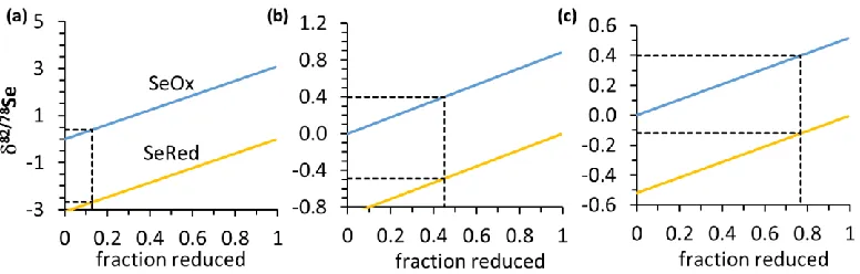
The assumed proportions and isotopic compositions of the three main sinks can further be used to derive an approximate average fractionation factor for oxyanion reduction (Fig. 5). If the initial selenium input to the ocean has a composition of 0‰, if modern seawater is close to +0.4‰ (i.e. the composition of manganese nodules with an assumed average adsorption fractionation of = 0.1‰, Table 3), and if the suboxic sink removes 13-77% of this dissolved reservoir (i.e. by partial reduction and preservation or organic matter), then one can calculate the minimum isotopic fractionation needed to raise the composition of the dissolved selenium from 0‰ to +0.4‰. Assuming an open-system behavior, the results suggest a minimum fractionation of 3.1‰ to 0.5‰; for a 45% suboxic inorganic sink, it would be 0.9‰ (Fig. 5). The corresponding reduced selenium that is produced during the reduction would fall between -2.7‰ and -0.1‰ (-0.5‰ for a 45% inorganic sink). These are minimum fractionations, because they assume that all of the selenium is inorganic. The data compilation above suggests a composition of -0.3 ± 0.4‰ for the suboxic open marine sink, but those sediments probably contain organic-bound selenide with a composition of perhaps +0.3‰ in addition to the isotopically light Se(0) and Se(-II) in pyrite (Table 2). This organic fraction ‘dilutes’ the bulk isotopic composition. Hence a fractionation factor equal to or slightly larger than 0.9‰ and 3‰, corresponding to an inorganic suboxic sink of between 13% and 45% of the total, is perhaps more plausible, because it would generate reduced inorganic selenium with compositions of -2.7‰ to -0.5‰ (or slightly lighter) that could balance the organic selenide. These inferred minimum fractionation factors fall within the range of values measured in natural microbial consortia (Ellis et al. 2003).
It is important to note that these calculations are based on a very limited amount of data, but they will hopefully inspire future studies to place more accurate constraints on the importance and internal complexities of the various selenium sources and sinks.
Implications and predictions
A mass balance as presented above (Table 4) allows formulating a number of testable hypotheses. First, it appears that partial oxyanion reduction in suboxic waters and sediments is responsible for raising the isotopic composition of selenium dissolved in seawater compared to its crustal source. This contrasts with the marine molybdenum cycle, where adsorption on ferromanganese oxides imparts the largest fractionation (Anbar 2004). However, it agrees well with observations from other redox-active elements such as sulfur or nitrogen, where the dissolved oxyanions are isotopically heavy due to partial reduction in sediments or oxygen-minimum zones (Canfield 2001; Sigman et al. 2009). If this inference is correct, then the isotopic composition of dissolved selenium should increase with an expansion of suboxic zones, at least up to a threshold where the oxyanion reservoir starts to become depleted.
13
compared to molybdenum (105 nM, 105-106 years) (Anbar 2004). Hence restricted basins such as the Black
Sea not only exchange water with the open ocean, but they are also strongly effected by local selenium sources and redox processes. This implies that euxinic sediments cannot be used as an archive of marine selenium compositions and the extent of oxic or suboxic bottom waters through time, as it is commonly done for molybdenum (e.g. Arnold et al. 2004). However, those sediments will provide a minimum estimate of local seawater values.
The composition of dissolved selenium in modern seawater may be best recorded by ferromanganese oxides, because the fractionation associated with adsorption is small (Table 3). Unfortunately, this proxy fails in the Precambrian, when the ocean was strongly stratified and Se(IV) may have been produced by Se(VI) reduction rather than organic remineralization (Schilling et al. 2014b; Stüeken et al. 2015d).
Despite the possibility of local heterogeneities, marine shales can record useful biogeochemical information, because, as noted above, where fractionations extend over a range larger than about 1‰, they are likely indicative of selenium oxyanion reduction and hence the presence of those ions somewhere in the ocean. This conclusion becomes significant in deep-time studies, because it implies that redox conditions somewhere on the surface of the Earth, either on land or in parts of the ocean or both, were high enough to oxidize selenium to Se(IV) or Se(VI). Given the high Eh of those species (Fig. 1), this reaction requires a strong oxidizer such as nitrate, manganese oxide or molecular oxygen. Evidence of selenium oxyanions can therefore help reconstruct redox changes over Earth’s history (e.g. Stüeken et al. 2015a). Furthermore, the absolute value of selenium isotopes in shales can inform about redox conditions in the overlying water column. If 8278S values are lighter than seawater, then non-quantitative oxyanion
reduction probably occurred in the water column or in sediments at the sampling locality. Conditions were thus probably oxic to suboxic (Stüeken et al. 2015c). If, on the other hand, shale values are generally positive, then partial reduction must have occurred elsewhere, and the residual isotopically heavy oxyanions were drawn down locally at this site, due to either enhanced productivity or strong anoxia or both. In most cases, the composition of local seawater is unknown; however, average crust can be used as a first-order calibration point, because the directions of isotopic fractionations in the selenium cycle make it unlikely that seawater would ever become lighter than the crust.
Lastly, the short marine residence time and possible heterogeneities of isotopic compositions in seawater forbid global extrapolations from single localities. Nevertheless, useful inferences can be made about presence or absence of oxidizing conditions in general (Stüeken et al. 2015a; Stüeken et al. 2015c).
Selenium isotopes in deep time
A few studies have investigated selenium isotopes in sedimentary rocks spanning the last 3.2 billion years (Rouxel et al. 2004; Mitchell et al. 2012; Layton-Matthews et al. 2013; Wen et al. 2014; Pogge von Strandmann et al. 2015; Stüeken et al. 2015a; Stüeken et al. 2015d; Stüeken et al. 2015c; Mitchell et al. 2016) (Fig. 6). The main findings in chronological order include:
14
2. An isotopic contrast between light non-marine (-0.28 ± 0.67 ‰) and heavy marine (+0.37 ± 0.27 ‰) shales in the late Archean Fortescue Group (Stüeken et al. 2015d): Light values down to -1.9‰ in the lacustrine Tumbiana Formation cannot be explained by Se(IV) adsorption or assimilation into biomass; they are most consistent with partial oxyanion reduction in lake sediments or the lake water column. Hence oxyanions were generated in non-marine environments around 2.7 Ga, supporting the interpretation of mild oxidative weathering at this time. Alkaline conditions in volcanic terrains (Stüeken et al. 2015b) could have contributed to oxyanion stability, because they are more soluble and adsorb much less strongly at high pH (Zinabu and Pearce 2003). Partial reduction of selenium oxyanions in these lacustrine and fluvial environments could have raised the isotopic composition of selenium that was transported into the ocean. This would explain the generally positive values found in marine black shales from open marine margins. Hence unlike today, the riverine input to the ocean was likely > 0‰ and the marine mass balance may have shifted towards more positive values. Marine hydrothermal sulfides of similar age are indistinguishable from the marine shales (Stüeken et al. 2015d) and also heavier than Phanerozoic hydrothermal deposits (Rouxel et al. 2004; Layton-Matthews et al. 2013), which is consistent with negligible amounts of dissolved selenium oxyanions in the Archean deep ocean.
3. A spike in selenium concentrations and isotopic ratios coincident with the 2.5 Gyr ‘whiff’ of oxygen (Stüeken et al. 2015a): The selenium spike occurs in marine black shales and coincides with an excursion in molybdenum abundances and isotopes (Anbar et al. 2007), suggesting that both elements were derived from the same source. Multiple lines of evidence point to a pulse of oxidative weathering of the continents and hence an enhanced flux of molybdenum, selenium and other elements to the ocean (Anbar et al. 2007; Reinhard et al. 2009; Kendall et al. 2015). Fractionation of selenium isotopes likely occurred during transport in rivers and estuaries or at the marine chemocline. Hence the complimentary light selenium reservoir that would have balanced the heavy black shales from this outer shelf section may be in shallower facies that were not preserved. It is unlikely to be in the deep ocean, if that was too anoxic to support a selenium oxyanion reservoir.
4. Marine selenium isotopic ratios above crustal average throughout the Proterozoic (Stüeken et al. 2015d; Mitchell et al. 2016): The ‘Great Oxidation Event’ around 2.4-2.3 Gyr (Lyons et al. 2014) is not obviously reflected in the selenium isotope and abundance record; Proterozoic marine shales are statistically indistinguishable from those of the Neoarchean. As before, partial reduction of selenium oxyanions produced during oxidative weathering may have retained light selenium in soils, rivers and estuaries, such that the average selenium flux into the ocean was isotopically heavy. Perhaps the reason for the lack of response to increasing atmospheric oxygen levels is that a large fraction of the weathered selenium was assimilated by the terrestrial biosphere and transported to the ocean as organic selenides, which did not participate in further redox reactions. However, some negative values from proximal black shales of the Mesoproterozoic Belt Supergroup (Stüeken et al. 2015d), as well as from Paleoproterozoic banded iron formations (Schilling et al. 2014b), indicate that perhaps selenium oxyanions did become more abundant in surface seawater, allowing for partial oxyanion reduction in the ocean. Analyses of non-marine sediments or a greater variety of marine facies may help resolve these questions.
15
al. 2014; Pogge von Strandmann et al. 2015; Stüeken et al. 2015d): With the oxygenation of the deep ocean in the Neoproterozoic or early Paleozoic (Lyons et al. 2014), selenium oxyanions probably became more stable, and something like a modern selenium cycle (Fig. 2) was established. This included non-quantitative oxyanion reduction in locally suboxic waters and sediments, i.e. in regions that were connected to the oxic selenium reservoir of the global ocean, leading to more negative selenium isotope values in marine shales. In-situ analyses of sedimentary pyrite grains show an increase of pyrite-bound selenium around the Precambrian-Cambrian boundary (Large et al. 2014), which further supports the idea of higher availability of selenium oxyanions for partial reduction to inorganic selenide. Prior to widespread ocean oxygenation, when pyrite-bound selenium levels were lower (Large et al. 2014), most selenium may have been preserved as organic-bound, because remineralization of organic matter was limited in the anoxic Precambrian ocean. Furthermore, a possible ‘second rise of oxygen’ in the Neoproterozoic atmosphere may have increased the total selenium flux coming from land. Chromium isotopes suggest that the redox state of weathering environments increased around 800 million years ago (Planavsky et al. 2014) to levels that would have been suitable for the production of Se(VI). Oxidative weathering in the earlier Precambrian may have stopped at Se(IV), i.e. the less oxidized form of selenium (Fig. 1). With higher selenium concentrations in seawater from the late Neoproterozoic onwards, hydrothermal oxyanion reduction could have also led to larger net fractionations (Rouxel et al. 2004; Layton-Matthews et al. 2013), which would explain why hydrothermal deposits of Phanerozoic age are much more fractionated than Neoarchean counterparts (Stüeken et al. 2015d) (Fig. 6). Restricted anoxic basins and regions of unusually high productivity, on the other hand, may tend to preserve positive values, presumably due to near quantitative selenium draw-down (Mitchell et al. 2012).
6. Negative excursions in selenium isotopes during the Permian-Triassic extinction and Ocean Anoxic Event 2 (Mitchell et al. 2012; Stüeken et al. 2015d): Net fractionations of selenium isotopes in black shales are usually not as negative as the reduced inorganic phases (Se(0), pyrite-bound Se(-II)) in them, because a large fraction of the selenium is contained in organic matter that does not carry the isotopic signature of dissimilatory oxyanion reduction (Stüeken et al. 2015c). Unusually light selenium isotope ratios down to < -0.5‰ are thus most likely the result of diminished selenium assimilation into biomass relative to the selenium supply. In the case of the Permian-Triassic extinction, selenium assimilation probably decreased as a direct consequence of ecosystem collapse (Stüeken et al. 2015c). As macro-organisms died out, the selenium demand and organic selenium export from the ocean probably dropped significantly. The ‘unused’ selenium oxyanions were thus subject to partial reduction in suboxic bottom waters. In the case of Ocean Anoxic Event 2, there is no sign of a productivity collapse, but the selenium supply by volcanism may have been unusually high, far exceeding the selenium demand by living organisms (Mitchell et al. 2012). Hence a relatively greater proportion of Se(IV) and Se(VI) may have been subject to dissimilatory reduction to inorganic reduced phases.
CONCLUSIONS AND FUTURE DIRECTIONS
16
uncertainties about the composition of the crust. The utility of this proxy could be advanced significantly with targeted studies of a greater range of igneous, metamorphic and sedimentary rocks, clarification of the isotopic composition of riverine, estuarine and marine waters, as well as with biological experiments at low selenium concentrations that mimic those in the modern ocean.
Sequential extraction of differing selenium phases from bulk rocks has the potential to reduce several uncertainties and should be pursued and perfected in future work. First, the organic selenium fraction could perhaps serve as a proxy for the composition of selenium dissolved in seawater as phytoplankton does today (Mitchell et al. 2012); second, the separation of organics from inorganic reduced phases such as Se(0) and pyrite-bound Se(-II) allows detecting the full range of fractionations imparted during reduction, thus circumventing the problem of phase mixing (Stüeken et al. 2015c); and third, the relative abundances of organic and inorganic phases can provide a measure of how much selenium was drawn into sediments by dissimilatory reduction versus assimilation versus adsorption. The relative proportions may be another proxy for selenium bioavailability.
Regarding the evolution of the selenium cycle, several topics still need to be addressed, such as the type and magnitude of selenium sources and sinks and their speciation in the Precambrian before the first and second rise of atmospheric oxygen, the bioavailability of selenium to ancient methanogens in the anoxic Archean ocean, the role of banded iron formations and dissolved ferrous iron in the selenium cycle, the importance of the rise of macro-biological productivity at the Precambrian-Cambrian boundary, and the onset of dimethyl selenide production. Studies involving multiple proxies alongside selenium isotopes may help answer some of these and other questions.
ACKNOWLEDGEMENTS
17
FIGURES
Figure 1: Eh-pH diagrams of (a) selenium, (b) sulfur, and (c) nitrogen. Acid-base transformations are
omitted for clarity. Roman numerals indicate oxidation states. Solid black lines mark the boundaries of liquid water stability. For nitrogen, solid lines represent nitrate-nitrite-ammonium equilibria, dashed lines and labels in parentheses represent nitrate-N2-ammonium equilibria. The figures were constructed with
18
Figure 2: Schematic of the modern marine Se cycle. Red arrows indicate reactions, blue arrows transport.
Fractionations and delta values are expressed in terms of 82Se/78Se in units of permil. *The minimum
fractionation of 1-3‰ for oxyanion reduction to inorganic reduced phases is derived from the mass balance described in the text. Fe(Mn)Ox-SeO32- denotes Se(IV) adsorption on ferromanganese oxides;
19
Figure 3: Testing for variations in mass dependence of selenium isotope fractionation. (a) Sulfur isotope
data spanning the last2 billion years, to exclude atmospheric effects. The slope of -7.7 is a biogenic feature (Ono 2008). (b) Sulfur isotope data from the Archean, showing the characteristic atmospheric slope around -1 (Zerkle et al. 2012). Sulfur data are compiled from the literature (Claire et al. 2014). Error bars for 33S are 0.02‰. (c) Post-Archean selenium isotope data, n = 140 (Stüeken et al. 2015d). (d) Archean
20
Figure 4: Proposed selenium mass balance for the modern ocean. The schematic was inspired by the
molybdenum cycle presented by Anbar (2004). Delta values are expressed in terms of 82Se/78Se in units of
21
Figure 5: Isotope fractionation model. Shown are the isotopic compositions of reduced inorganic
[image:21.612.76.464.88.212.2]22
Figure 6: Selenium abundances (a) and isotopes (b) through time. The thin dashed line marks the crustal
23
[image:23.612.94.518.231.331.2]TABLES
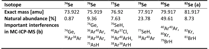
Table 1: Stable selenium isotopes. Abundances and exact masses are taken from Fernández-Martínez &
Charlet (2009), interferences are taken from Stüeken (2013). (a) 82Se decays with a half-life (t 1/2) of
1.08∙1020 years, which makes it stable for practical purposes. Other unstable isotopes (72Se, t
1/2 = 8.4 days; 75Se, t
1/2 = 120 days; 79Se, t1/2 = 295,000 years) are omitted. (b) Not included are potential isobaric
interferences with doubly-charged heavy metals and metal oxides (cf. Layton-Matthews et al. 2006), for which there is no experimental evidence in MC-ICP-MS, the most common analytical technique (Stüeken et al. 2013).
Isotope 74Se 76Se 77Se 78Se 80Se 82Se (a)
Exact mass [amu] 73.922 75.919 76.92 77.917 79.917 81.917
Natural abundance [%] 0.87 9.36 7.63 23.78 49.61 8.73
Important interferences
in MC-ICP-MS (b) 74Ge,
36Ar38Ar
76Ge, 36Ar40Ar, 38Ar38Ar, 75AsH
76SeH, 40Ar37Cl, 36Ar40ArH, 38Ar38ArH
77SeH, 38Ar40Ar
40Ar40Ar, 80Kr, 79BrH
24
Table 2: Concentrations and isotopic compositions of selenium in various reservoirs. blank cells = not determined; n = number of samples. (a)
1
concentrations are in ppb [ng/g] unless noted otherwise. (b) isotopic data are in units of permil. (c) average of basalt and diorite. (d) FeMn oxides 2
denotes ferromanganese crusts and nodules from the modern ocean. (e) black smokers reflect high-temperature fluids of marine hydrothermal 3
vents; low-temperature fluids are undetermined. (f) shale includes Precambrian and Phanerzoic samples. Precambrian data may be biased towards 4
more positive 82/78Se values relative to average crust, as discussed in the text. (g) average selenium concentration of upper crust is calculated
5
following the recipe of Condie (1993) or Wedepohl (1995). References: 1. Dreibus et al. (1993), 2. DuFresne (1960), 3. Edgington & Byers (1942), 6
4. Floor & Roman-Ross (2012), 5. Goldschmidt & Storck (1935), 6. Greenland (1967). 7. Hertogen (1980), 8. Johnson & Bullen (2004b), 9. Koljonen 7
(1973b), 10. Koljonen (1973a), 11. Kulp & Pratt (2004), 12. Lorand et al. (2003), 13. Marin et al. (2001), 14. Mitchell et al. (2012), 15. Schirmer et 8
al. (2014), 16. Shore (2010), 17. Wen et al. (2014), 18. Stüeken et al. (2015d), 19. Stüeken et al. (2015a), 20. Tamari et al. (1990), 21. Tischendorf 9
(1959), 22. Turekian & Wedepohl (1961), 23. Wang et al. (2013), 24. Rouxel et al. (2002), 25. Schilling et al. (2014b), 26. Takematsu et al. (1990), 10
27. Schilling et al. (2011b), 28. Wedepohl (1995), 29. Conde & Alejos (1997), 30. Plant (2014), 31. Cutter & Cutter (2001), 32. Wen & Carignan 11
(2007), 33. Mosher & Duce (1987), 34. Haygart et al. (1994), 35. von Damm (1990), 36. Condie (1993). 12
13
Type Geom. mean
[ppb] (a)
[ppb] (a) n
ref. for
concentrations
82/78Se
(b)
(b) n
ref. for isotopes geological reservoirs:
chondritic meteorites 9,580 +6,548/-3,889 96 1, 2, 6, 23
iron meteorites 22,361 +67,264/-16,782 4 24 +0.11 ±0.34 4 24
upper mantle 27 +61/-19 140 9, 12, 20, 23 +0.15 1 24
gabbro 97 +137/-57 17 9, 13, 20
basalt 57 +126/-39 47 7, 9, 13, 20 +0.36 ±0.13 4 24
andesite 7 +23/-6 19 9, 13, 20
diorite 68 +81/-37 14 9, 13, 20 -0.33 1 24
granodiorite 21 +61/-16 14 9, 13, 20
granite 18 +46/-13 59 9, 13, 20
rhyolite 15 +65/-12 14 9, 13, 20
shale (f) 1,189 +4,765/-952 646
3, 8, 11, 14, 16, 17, 18, 19, 20, 21
+0.09 ±0.60 522
14, 16, 17, 18, 19
sandstone 42 +80/-28 16 10, 20, 22
carbonate 116 +590/-97 23 10, 15, 20, 22 +0.14 ±0.41 2 24
FeMn oxides (d) 580 +1,176/-389 71 5, 15, 26 +0.32 1 24
Precambrian BIF 79 +77/-39 12 15 < 0? 25
25
gneiss 77 +147/-51 23 10
serpentine 291 +1,516/-244 5 10, 13
amphibolite 217 +163/-93 6 10
schist 1,007 +7,333/-885 14 10
→ upper crust (g) 34 or 59 +137/-41 after 36 or 28 +0.01 ±0.49 24 (c)
other environmental reservoirs:
seawater 1-2 nM 30, 31 ≥ +0.3 0 14, 24
river water 0.1-25.3 nM, avg. 2.17 nM, Amazon 2.66 nM 29, 30 ~ 0? 0 18
geothermal water 25-6000 nM, black smokers 73 ± 21 nM (e) 4, 35
atmospheric particulates 0.0045-1.34 ng/m^3 32, 33, 34 < 0? 0 27
atmospheric gas 0.0003-0.35 ng/m^3 32, 33, 34 < 0? 0 27
marine biomass 1.7-5.6 mol selenium/mol carbon 14 ~ +0.3 1 14
26
Table 3: Low-temperature isotopic fractionations. The fractionation between reactant (R) and product
18
(P) of a reaction is defined as R-P 1000∙(R-P -1), where R-P = (82Se/78Se)R/(82Se/78Se)P. R-P approximately
19
equal to 82/78Se
reactant - 82/78Seproduct; the difference is < 0.1‰ for R-P ≤ 20‰. Note that most experiments
20
were conducted with much higher selenium concentrations than found in most natural environments, 21
where fractionations may generally be smaller (Ellis et al. 2003). References: 1. Johnson et al. (1999), 2. 22
Johnson & Bullen (2003), 3. Johnson & Bullen (2004b), 4. Rees & Thode (1966), 5. Rashid & Krouse (1985), 23
6. Krouse & Thode (1962), 7. Mitchell et al. (2013), 8. Herbel et al. (2000), 9. Ellis et al. (2003), 10. Herbel 24
et al. (2003), 11. Schilling et al. (2011b), 12. Schilling et al. (2013), 13. Clark & Johnson (2010). 25
26
Pathway 82Se/78Se) references
reduction:
abiotic Se(VI) → Se(IV) 5.6‰ to 11.8‰ 1, 2, 4 abiotic Se(IV) → Se(0) 4.6‰ to 11.2‰ 4, 5, 6, 7 biotic Se(VI) → Se(IV) 0.2‰ to 5.1‰ 8, 9 biotic Se(IV) → Se(0) 1.1‰ to 8.6‰ 8, 9, 10 (a-)biotic Se(0) → Se(-II) < 0.5‰ 3
oxidation:
(a-)biotic Se(-II) → Se(0) < 0.5‰ 1, 3 (a-)biotic Se(0) → Se(IV) < 0.5‰ 1, 3 (a-)biotic Se(IV) → Se(VI) < 0.5‰ 1, 3
adsorption:
Se(IV) on FeMn-Oxide <0.1‰ 7
Se(VI) on FeMn-Oxide < 0.7‰, average ~0.1‰ 7
volatilization:
Se(IV)/(VI) → CH3-Se(-II) 2‰ to 4‰ 11, 12 assimilation:
Se(IV)/(VI) → org. Se(-II) <0.6‰ 13 27
27
Table 4: Modern ocean mass balance. Sink fluxes were calculated as fractions of the total input, assuming
29
the same relative proportions as in the molybdenum cycle (Little et al. 2015). Isotopic compositions of 30
sinks were calculated by taking the average of averages of different basins to avoid bias towards larger 31
datasets. References for isotopic data are given in the text. Fluvial and hydrothermal fluxes were 32
calculated by multiplication of average concentrations in mol/liter from Conde & Alaejos (1997, ref. 1) 33
and von Damm (1990, ref. 2), respectively, with the corresponding average water fluxes in liters/year 34
(Emerson and Hedges 2008, ref. 3). Atmospheric input is taken from Mosher & Duce (1987). 35
36
average flux 82/78Se ref. for fluxes
Sources [measured]:
Rivers 8∙107 mol/yr n.d. 1, 3
Volcanoes 1∙107 mol/yr n.d. 4
Hydrothermal vents 4∙105 mol/yr n.d. 2, 3
Total sources 9∙107 mol/yr ~ 0?
Sinks [inferred from steady state assumption and Mo equivalents]:
FeMnOxide adsorption 4.3∙107 mol/yr +0.32 ± 0.20 48% of total
Restr. euxinic basins 0.6∙107 mol/yr +0.08 ± 0.05 7% of total
Local suboxia 4.1∙107 mol/yr -0.29 ± 0.41 45% of total
Total sinks 9∙107 mol/yr +0.03 ± 0.28 mass balance
28
REFERENCES
40 41
Algeo TJ, Lyons TW (2006) Mo–total organic carbon covariation in modern anoxic marine environments: 42
Implications for analysis of paleoredox and paleohydrographic conditions. Paleoceanography 43
21:doi:10.1029/2004PA001112 44
Amouroux D, Liss PS, Tessier E, Hamren-Larsson M, Donard OFX (2001) Role of oceans as biogenic sources 45
of selenium. Earth and Planetary Science Letters 189:277-283 46
Anbar AD (2004) Molybdenum stable isotopes: observations, interpretations and directions. Reviews in 47
Mineralogy and Geochemistry 55:429-454 48
Anbar AD, Duan Y, Lyons TW, et al. (2007) A whiff of oxygen before the Great Oxidation Event? Science 49
317:1903-1906 50
Arnold GL, Anbar AD, Barling J, Lyons TW (2004) Molybdenum isotope evidence for widespread anoxia in 51
mid-Proterozoic oceans. Science 304:87-90 52
Aurelio G, Fernandez-Marinez A, Cuello GJ, Roman-Ross G, Alliot I, Charlet L (2010) Structural study of 53
selenium (IV) substitution in calcite. Chemical Geology 270:249-256 54
Balistrieri LS, Chao TT (1990) Adsorption of selenium by amorphous iron oxyhydroxide and manganese 55
dioxide. Geochimica et Cosmochimica Acta 54:739-751 56
Banuelos GS, Lin Z-Q, Yin X (2013) Selenium in the Environment and Human Health. CRC Press 57
Bar-Yosef B, Meek D (1987) Selenium sorption by kaolinite and montmorillonite. Soil Science 144:11-19 58
Basaglia M, Toffanin A, Baldan E, Bottegal M, Shapleigh JP, Casella S (2007) Selenite-reducing capacity of 59
the copper-containing nitrite reductase of Rhizobium sullae. FEMS Microbiology Letters 269:124-60
130 61
Birringer M, Pilawa S, Flohé L (2002) Trends in selenium biochemistry. Natural product reports 19:693-62
718 63
Boeck A, Rother M, Leibundgut M, Ban N (2006) Selenium metabolism in prokaryotes. In: Selenium - Its 64
molecular biology and role in human health. Hatfield DL, Berry MJ, Gladyshev VN, (eds). Springer, 65
New York 66
Canfield DE (2001) Biogeochemistry of sulfur isotopes. Reviews in Mineralogy and Geochemistry 43:607-67
636 68
Carignan J, Wen H (2007) Scaling NIST SRM 3149 for Se isotope analysis and isotopic variations of natural 69
samples. Chemical Geology 242:347-350 70
Chasteen TG, Bentley R (2003) Biomethylation of selenium and tellurium: microorganisms and plants. 71
Chemical Reviews 103:1-26 72
Chau YK, Wong PTS, Silverberg BA, Luxon PL, Bengert GA (1976) Methylation of selenium in the aquatic 73
environment. Science 192:1130-1131 74
Claire MW, Kasting JF, Domagal-Goldman SD, Stüeken EE, Buick R, Meadows VS (2014) Modeling the 75
signature of sulfur mass-independent fractionation produced in the Archean atmosphere. 76
Geochimica et Cosmochimica Acta 141:365-380. 77
Clark SK, Johnson TM (2008) Effective isotopic fractionation factors for solute removal by reactive 78
sediments: a laboratory microcosm and slurry study. Environmental Science and Technology 42 79
Clark SK, Johnson TM (2010) Selenium stable isotope investigation into selenium biogeochemical cycling 80
in a lacustrine environment: Sweitzer Lake, Colorado. Journal of Environmental Quality 39:2200-81
2210 82
Conde JE, Alaejos MS (1997) Selenium concentrations in natural and environmental waters. Chemical 83
Reviews 97:1979-2003 84
Condie KC (1993) Chemical composition and evolution of the upper continental crust: contrasting results 85
from surface samples and shales. Chemical Geology 104:1-37 86