ISSN Print: 2160-8881
DOI: 10.4236/opj.2019.98B002 Aug. 9, 2019 11 Optics and Photonics Journal
An Improved Algorithm for 3D Reconstruction
Integration Based on Stripe Reflection Method
Xu Gao, Peiji Guo
*School of Optoelectronic Science and Engineering, Key Lab of Advanced Optical Manufacturing Technologies of Jiangsu Province and Key Lab of Modern Optical Technologies of Education Ministry of China, Soochow University, Suzhou, China
Abstract
This paper introduces the basic principle of stripe reflection method and proposes an improved algorithm on the traditional Southwell gradient itera-tive integration algorithm. The algorithm adds a coefficient value with an at-tenuation factor to the compensation height value and the value of the atten-uation factor is changed by the determination of the compensation height threshold. Through computer simulation, the fitting error of the recon-structed surface show that the RMS of the new method is one order of mag-nitude better than the traditional algorithm and the PV value of the high fre-quency part is about 1/15 of the traditional algorithm. It is proved that the improved algorithm can effectively improve the convergence and noise resis-tance of the iterative algorithm.
Keywords
Stripe Reflection Method, Gradient Iterative Integration, Fitting Error
1. Introduction
The fringe reflection method [1] is based on the simple principle of light reflec-tion. The method has the advantages of simple structure, high sensitivity, large dynamic range, and is generally used for full-caliber testing of the aspherical surface shape during the rough polishing stage. Many experts and scholars have carried out many researches and practices on this technology. Su Peng et al. of the University of Arizona in the United States proposed a SCOTS testing me-thod and successfully detected the 8.2 m GMT sub-mirror through high-precision calibration [2] [3]. The Sichuan University [4] [5] and the Chi-nese Academy of Sciences [6] have done a lot of research on the stripe reflection
How to cite this paper: Gao, X. and Guo, P.J. (2019) An Improved Algorithm for 3D Reconstruction Integration Based on Stripe Reflection Method. Optics and Photonics Journal, 9, 11-19.
https://doi.org/10.4236/opj.2019.98B002 Received: July 19, 2019
DOI:10.4236/opj.2019.98B002 12 Optics and Photonics Journal technology and have achieved certain results. This paper introduces the basic principle of the stripe reflection method and introduces an iterative algorithm based on the Southwell integration method. Then we propose a compensation algorithm with attenuation factor parameters based on the traditional iterative integration. The computer simulation results show that the new method has better convergence in a single iteration compared with the traditional method. The algorithm for changing the coefficient has a better fitting result than the al-gorithm without changing the coefficient, and verifies the superiority of the im-proved algorithm.
2. The Basic Principle of the Stripe Reflection Method
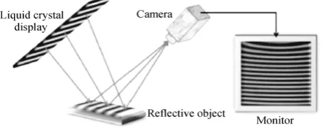
The measurement model is shown in Figure 1. The computer produces a stan-dard sinusoidal stripe that transmits the encoded fringe image onto the LCD screen. The stripe displayed on the screen is projected onto the reflective surface. The deformed fringe image is captured by a CCD camera, which records the gradient and height of each reflective point on the reflective surface.
The intensity of each point on the deformed fringe pattern after reflection by the mirror to be tested can usually be expressed as:
( , ) ( , ) ( , )cos[ ( , ) ]
n n
I x y =a x y b x y+ ϕ x y +σ (1) where I x yn
(
,)
is the light intensity of each point of the stripe diagram,(
,)
a x y is the background light intensity, b x y( , ) is amplitude modulation, and ϕ
(
x y,)
is the phase modulation to be solved, and σn is the additional phase, which is determined when the fringes are generated. The computer gen-erated grating can accurately control the magnitude of the single phase shift. The calculation of the phase modulation ϕ(
x y,)
is shown in Equation (2)1 1
1
( , )sin
( , ) tan , 1,2,...,
( , )cos
N
n n
n N
n n
n
I x y
x y n N
I x y σ ϕ
σ
− −
−
= − =
∑
∑
(2) [image:2.595.261.491.615.706.2]The arctangent function obtains the truncated phase of [−π, π). In order to de-termine the one-to-one correspondence between the pixel of the screen and the pixel of the mirror, it is necessary to expand the phase to form a continuous phase. The method of phase unwrapping includes the spatial phase expansion method [7] [8] and time phase expansion method [9] [10]. The former mainly
DOI: 10.4236/opj.2019.98B002 13 Optics and Photonics Journal includes branch cutting method, quality map guiding method, minimum norm method; the latter mainly includes binary encoding and multi-frequency hete-rodyne method.
3. Gradient Integral Algorithm Analysis
Measuring the surface of the object by the stripe reflection system, we can obtain two gradient distributions in the mutually perpendicular direction. The gradient refers to the partial derivatives g x yx( , ) and g x yy( , ) obtained by the height
( , )
z x y of the surface in the directions of x and y. The calculation is as shown in Equation (3) and Equation (4):
( , ) ( , )
x z x y
g x y
x
∂ =
∂ , (3)
( , ) ( , )
y z x y
g x y
y
∂ =
∂ , (4)
In order to obtain the specular surface 3D height information, we need to in-tegrate the derivative:
( , ) x y
z x y =
∫
g dx+∫
g dy, (5)In the actual testing process, the gradient field is not a conservative field due to the influence of system error and image noise. Southwell model based on re-gional wave front reconstruction method can not only effectively suppress noise but also deal with complex connected regions. Therefore, it has become the mainstream algorithm of gradient integral.
3.1. Southwell Model Algorithm
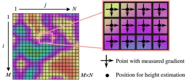
The Southwell grid model is shown in Figure 2. The matrix size is M × N. The solid black dot in the graph represents the height point and the arrow represents the gradient direction of the point x, y. The average of two adjacent gradient values is equal to the ratio of the difference in height to the pixel width (h).
The gradient matrix is the same size as the height matrix. The relationship between the gradient data and the height data is only related to the same row or the same column. The above relationship is expressed as
(
)
(
)
, 1 , , 1 ,
1, , 1, ,
1 1 ( ) 1,2,..., ; 1,2,..., 1
2
1 1 ( ) 1,2,..., 1; 1,2,...,
2
x x
i j i j i j i j
y y
i j i j i j i j
g g z z i M j N
h
g g z z i M j N
h
+ +
+ +
+ = − = = −
+ = − = − =
(6)
Z represents a height matrix, the size is MN × 1; D represents a coefficient matrix, which is a sparse matrix size [(M − 1)N + M(N − 1)] × MN; G represents a gradient matrix, and the size [(M − 1)N + M(N − 1)] × 1. Equation (6) can be rewritten into:
DOI:10.4236/opj.2019.98B002 14 Optics and Photonics Journal Figure 2. Southwell grid model.
D, and the least norm solution of Z can be obtained by using the least square method:
(
T)
1 Tf f f
Z = D D − D G. (8)
3.2. Improved Iterative Algorithm Based on Southwell Model
The rate of convergence and the ability to suppress noise in the late iteration are two conditions for evaluating the merits of an iterative algorithm. Especially for large-caliber mirrors, the gradient data needs to be reprocessed for each itera-tion. The higher the convergence efficiency, the fewer the number of iterations. As the number of iterations increases, the ability to suppress gradient noise in the iteration ensures the accuracy of the final fitted shape.The traditional iterative algorithm is showed as follows [11]
1) Using the traditional integration method to obtain the original surface height z x y0( , ) as the initial value of the iteration;
2) Calculate the derivatives q x y( , ) and p x y( , ) of the current height
( , )
n
z x y in the x and y directions, and make a difference with the original gra-dient to obtain gragra-dient residuals dg x yx( , ) and dg x yy( , );
3) Using traditional integration method to integrate dg x yx( , ) and ( , )
y
dg x y to obtain the compensation height value n( , )
c
z x y ; 4) The compensated height values n
(
,)
n1(
,)
n( , ) /c k
z x y =z − x y +z x y n , nk = 3, 4.0909, 4.9476, 5.6768 (k = 1, 2, 3, 4);
5) Repeat the iterative process of 2-4 until the iterations of adjacent two itera-tions are less than the threshold, maxzn−zn−1 < threshold.
This section presents an improved algorithm that includes two improvements. First, use the two variables of attenuation factor t and iteration number n to control the contribution value of the compensation height to participate in the iteration. Second, the threshold is set for the nth compensation height during iteration. The formula of the new iterative algorithm can be written as:
1
( , ) ( , ) ( , )
n n n
c
z x y =z − x y + ⋅ω z x y , (9) 1
(n 1)t
ω=
DOI: 10.4236/opj.2019.98B002 15 Optics and Photonics Journal The height of the nth compensation is related to the height threshold:
( )
threshold RMSm
n c
z
n
<
⋅ , (11)
The value of m is generally between [1] [5], Coefficient ω determines the weight of the compensation height value to participate in the iteration. In the in-itial stage of the iteration, a smaller t can increase the convergence rate. With the progress of iteration, in order to reduce excessive noise participation in the iteration, we set the RMS threshold of the nth compensation height. If it is larger than the threshold value, the value of attenuation factor t is increased to pre-vent excessive noise data in the compensation height from affecting the fitting results. Through computer simulation, the traditional algorithm and the im-proved algorithm iteratively integrate the gradient data obtained by the stripe reflection measurement system, and analyze the wavefront reconstruction accu-racy.
4. Computer Simulation
The simulated face is divided into two parts: z1 is the standard paraboloid:
2 2
1 50 50x y
z = + , (12)
2
z is set to a high-order shape in a certain area:
2 2 6 4 4 2 5 2
1
0.5cos ( ) (0.25(0.5 2) 2) 0.125((0.5 ) 2) z
x y x y
=
+ + − + + + , (13)
The size of z1 and z2 is 501 × 501 pixels, and the pixel size is 0.04 mm. In order to get closer to the actual testing conditions, we combined the gradient data of surface shape with the gaussian noise whose SNR = 100:1. Using the tra-ditional Southwell integral z0 as the initial shape, after four iterations we com-pare the high frequency partial fit results on the green lines in Figure 3. The si-mulation results are shown in Figure 4.
In order to compare the capability of the three iterative methods to iterative errors in the high-frequency part, we gather the high-frequency errors fitted by the three methods into the same figure, as shown in Figure 5, and list the RMS of the four iterations, as shown in Table 1.
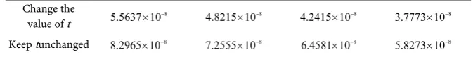
In order to verify the effect of controlling the attenuation factor by setting compensation high threshold in the later iteration, we will perform 10 iterations without changing the initial attenuation coefficient t and controlling the attenu-ation coefficient, and compare the rms results of the last four fittings. The result is shown in Figure 6. The height average of the last four compensations is shown in Table 2.
5. Summary and Discussion
DOI:10.4236/opj.2019.98B002 16 Optics and Photonics Journal
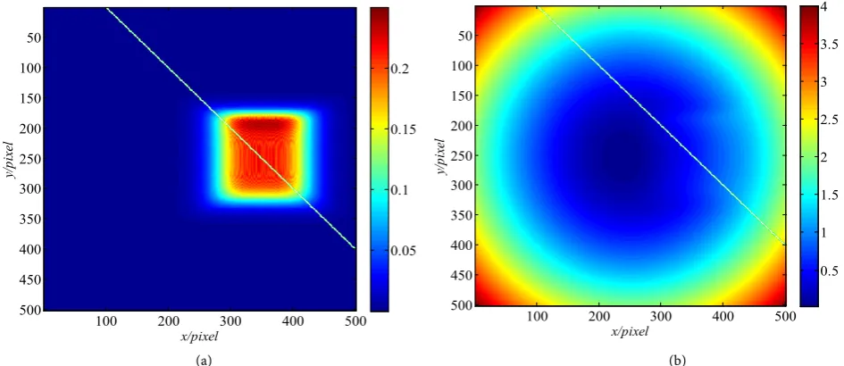
[image:6.595.62.535.71.276.2](a) (b)
Figure 3. The simulation surface shape. (a) The two-dimensional shape of z2, (b) Two-dimensional shape synthesized by z1
and z2.
(a) (b)
(c) (d)
x/pixel
y/
pi
xe
l
100 200 300 400 500
50 100 150 200 250 300 350 400 450 500 0.05 0.1 0.15 0.2 x/pixel y/ pi xel
100 200 300 400 500
50 100 150 200 250 300 350 400 450 500 0.5 1 1.5 2 2.5 3 3.5 4 x/pixel y/ pi xe l
100 200 300 400 500
50 100 150 200 250 300 350 400 450 500 -3.5 -3 -2.5 -2 -1.5 -1 -0.5 0 0.5 1 x 10⁻⁵
100 200 300 400 500
-1.5 -1 -0.5 0 0.5 1 1.5 x 10⁻⁵
x/pixel Erro r/m m x/pixel y/ pi xe l
100 200 300 400 500
50 100 150 200 250 300 350 400 450 500 -2.5 -2 -1.5 -1 -0.5 0 0.5 1 1.5 2 x 10⁻⁵
100 200 300 400 500 600
-6 -4 -2 0 2 4 6 x 10
-6
x/pixel
Erro
r/m
X. Gao, P. J. Guo
DOI: 10.4236/opj.2019.98B002 17 Optics and Photonics Journal
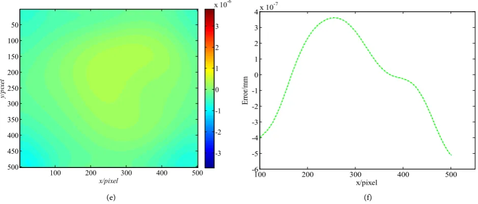
[image:7.595.67.537.74.275.2](e) (f)
[image:7.595.213.536.351.469.2]Figure 4. Gradient integral method reconstruction error and high frequency fitting error. (a) Traditional Southwell integral sur-face residual error, (b) Traditional Southwell integral high frequency line fitting error, (c) Traditional iterative integral sursur-face residual error, (d) Traditional iterative integration high frequency line fitting error, (e) Improved surface residual error of iterative integration, (f) Improved iterative integral high frequency line fitting error.
Figure 5. Comparison of high-frequency line error distribution.
Figure 6. Root mean square error comparison.
integration. The algorithm uses the attenuation coefficient to control the com-pensation value and the attenuation coefficient t is controlled by the compensa-tion height threshold. Through computer simulacompensa-tion, it is verified that the algo-rithm has better convergence rate in the early iteration period and better fitting x/pixel
y/
pi
xe
l
100 200 300 400 500
50
100 150
200 250 300 350
400 450
500
-3 -2 -1 0 1 2 3 x 10⁻⁶
100 200 300 400 500
-6 -5 -4 -3 -2 -1 0 1 2 3 4 x 10⁻⁷
x/pixel
Erro
r/m
m
100 200 300 400 500
x(pixel)
-1.5 -1 -0.5 0 0.5 1 1.5
Height error(mm)
10-5
Southwell integration method Traditional iterative integration Improved iterative integration Zero baseline
7 8 9 10
Iterative times
0.8 0.9 1 1.1 1.2 1.3
Std. of error in Z(mm)
10-7
[image:7.595.215.532.508.628.2]DOI:10.4236/opj.2019.98B002 18 Optics and Photonics Journal Table 1. The error size of single iteration reconstruction in iteration process.
Table Head Southwell integration RMS(mm)
method Traditional iterative integration Improved iterative integration Initial value 1.2472 10× −5 1.2472 10× −5 1.2472 10× −5
1st iteration - 6.2299 10× −6 1.9712 10× −6
2nd iteration - 4.7936 10× −6 7.4142 10× −7
3rd iteration - 3.8844 10× −6 3.6974 10× −7
[image:8.595.203.540.248.289.2]4th iteration - 3.2445 10× −6 2.2140 10× −7
Table 2. The average compensation height of the last four iterations (mm).
Change the
value of t 5.5637 10× −8 4.8215 10× −8 4.2415 10× −8 3.7773 10× −8 Keep tunchanged 8.2965 10× −8 7.2555 10× −8 6.4581 10× −8 5.8273 10× −8
of high frequency detail. In the latter part of the iteration, by changing the size of
t, it can effectively prevent too many noise points from participating in the itera-tion and leading to poor surface performance. The simulaitera-tion results show that the improved algorithm effectively suppresses the influence of noise and has better fitting accuracy than the traditional algorithm at low SNR.
Funding
Supported by the NSFC (NO.61378055), Advantages of disciplines in colleges and universities in Jiangsu Province construction grant program.
Conflicts of Interest
The authors declare no conflicts of interest regarding the publication of this pa-per.
References
[1] Hung, Y.Y., Lin, L., Shang, H.M., et al. (2000) Practical Three-Dimensional Com-puter Vision Techniques for Full-Field Surface Measurement. Opt. Eng., 39, 143-149.https://doi.org/10.1117/1.602345
[2] Su, P., Parks, R.E., Wang, L.R., et al. (2010) Software Configurable Optical Test Sys-tem: A Computerized Reverse Hartmann Test. Applied Optics, 49, 4404–4412.
https://doi.org/10.1364/ao.49.004404
[3] Huang, R., Su, P. and Burgea, J.H. (2015) Deflectometry Measurement of Daniel K. Inouye Solar Telescope Primary Mirror. Proceedings of the SPIE, 9575, Article ID: 957515.
[4] Zhao, W.C., Fan, B., Wu, F., et al. (2013) Experimental Analysis of Reflector Test Based on Phase Measuring Deflectometry. Acta Optica Sinica, 33, Article ID: 0112002. https://doi.org/10.3788/aos201333.0112002
DOI: 10.4236/opj.2019.98B002 19 Optics and Photonics Journal [6] Wang, H.R., Li, B., Wang, Z.F., et al. (2013) Plane Measurement of Trough Parabol-ic Element Mirror Based on Stripe Reflection Method. Acta Optica Sinica, 33, Ar-ticle ID: 0112007.
[7] Strand, J., Taxt, T. and Jain, A.K. (1999) Two-Dimensional Phase Unwrapping Us-ing a Block Least-Square Method. IEEE Tran. Image Process, 8, 375-386.
https://doi.org/10.1109/83.748892
[8] Goldstein, R.M., Zevker, H.A. and Werner, C.L. (1988) Statellite Radar Interferome-try: Two-Dimensional Phase Unwrapping. Radio Science, 23, 713-720.
https://doi.org/10.1029/rs023i004p00713
[9] Strand, J., Taxt, T. and Jain. A.K. (1999) Two-Dimensional Phase Unwrapping Us-ing a Block Least-Square Method. IEEE Tran. Image Process, 8: 375-386.
https://doi.org/10.1109/83.748892
[10] Huntley, J.M. and Saldner, H.O. (1993) Temporal Phase-Unwrapping Algorithm for Automated Interferogram Analysis. Applied Optics, 32, 3047-3052.
https://doi.org/10.1364/ao.32.003047
[11] Huang, L. and Asundi, A. (2012) Improvement of Least-Squares Integration Method with Iterative Compensations in Fringe Reflectometry. Applied Optics, 51, 7459-7465.