Abstract — The new approach proposed by the authors in this paper consists of implementing friction pendulums having the sliding surface profile based on a polynomial function of superior order. This seismic isolation system permits, for each surface, a greater flexibility in controlling the oscillations of the upper structure, in terms of displacements or dissipated energy, by using three parameters to control the force-displacement relation.
Index Terms—isolation system, dissipated energy, friction
pendulum, finite element analysis
I. INTRODUCTION
or safety and integrity reasons against earthquakes, effective and reliable techniques are desired. The optimum solution against earthquake effects is to control and limit the transfer of energy from the ground to a superstructure that means to dissipate this energy [1].
For these reasons, the actual trend is represented by using the friction pendulum. This is a sturdy passive device, capable to sustain significant loads and to assure the control of oscillating structures [2].
Friction pendulums can be classified, according to the number of sliding surfaces, in mono-armature or multi-armature [3]. While classical friction pendulum bearings contain one or more cylindrical or spherical sliding surfaces, each having a radius of curvature R and friction coefficient µ, they provide just pairs of two parameters controlling the dynamic behaviour of a structure isolated by this kind of device. The friction pendulum system with one concave spherical shaped sliding surface is presented in [4] while the
Manuscript received March 18, 2012; revised April 16, 2012.
This work was supported in part by the Managing Authority for Sectorial Operational Program for Human Resources Development (MASOPHRD), within the Romanian Ministry of Labor, Family and Equal Opportunities by co-financing the project “ Doctoral Scholarships investing in research-development-innovation for the future (DocInvest) ” POSDRU/107/1.5/S/76813.
A. A. Minda is with the Economical Engineering Department, “Eftimie Murgu” University of Resita, 320085 Romania. (e-mail: [email protected]).
G. R. Gillich is with the Mechanical Engineering Department, “Eftimie Murgu” University of Resita, 320085 Romania. (e-mail: [email protected]).
C. M. Iavornic is with the Mechanical Engineering Department, “Eftimie Murgu” University of Resita, 320085 Romania. (e-mail: [email protected]).
P. F. Minda is with the Mechanical Engineering Department, “Eftimie Murgu” University of Resita, 320085 Romania. (e-mail: [email protected]).
double concave bearing was presented in [5].
A new base isolator, called a variable curvature friction pendulum system, was introduced by Tsai , Chiang and Chen in [6]. The difference between the variable curvature friction pendulum system and the friction pendulum system is that the isolator’s radii can be lengthened with the increase of the isolator displacement. Pranesh and Sinha introduced in [7] and [8] a variable curvature friction pendulum system with the sliding surface based on an ellipse. The major axis of the ellipse can be lengthened with increase of sliding displacement. They have made analysis in terms of behaviour of the isolated structure, without being analyzed the behaviour of the friction pendulum itself.
The new approach proposed by the authors in this paper consists of implementing friction pendulums having the sliding surface profile based on a polynomial function of superior order. This seismic isolation system permits, for each surface, a greater flexibility in controlling the oscillations of the upper structure, in terms of displacements or dissipated energy, by using three parameters to control the force-displacement relation. Namely, these parameters are the friction coefficient µ, and two characteristic values of the curve on which the sliding surface is constructed.
Opposite to classical systems, where the contact between the slider and the sliding surface assured almost uniformly distributed contact stress even for metallic components, the new devices make use of an elastic element between the slider and the sliding surface. A quasi-uniform pressure distribution on the sliding surface can be obtained in this way. Static and dynamic analyses were performed using the finite element method confirming that the use of an elastomeric element is suitable for this purpose.
II. MATHEMATICAL MODEL OF SIMPLE FRICTION PENDULUM WITH SLIDING SURFACES GENERATED BY
POLYNOMIAL FUNCTIONS
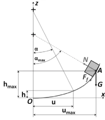
In the case of the simple friction pendulum, with cylindrical or spherical sliding surface, the control of the movement can be made with two parameters: the radius of the pendulum R and the friction coefficient.
The height variation h expressed in terms of and then in terms of displacement u, is:
Analytical and Finite Element Study for Friction
Pendulum with Parameterized Sliding Surfaces
Andrea Amalia Minda, Member, IAENG, Gilbert-Rainer Gillich Member, IAENG, Claudiu Mirel Iavornic, Member, IAENG and Petru Florin Minda, Member, IAENG
1 cos
1 cos arcsinuh R R
R
(1)
The friction force value is
fF N sign u (2) The signum function is equal to -1 or +1 depending on whether u is negative or positive, respectively. If we consider the motion in the positive direction of Ox axis, we can take sign u
1, so Ff expressed in terms of iscos f
[image:2.595.337.521.97.307.2]F G , where G is the vertical loading resulting from the structure.
Fig. 1. A simple friction pendulum scheme with the forces acting on circular sliding surface
On the interval
0,umax
the dissipated energy due to friction is:
max
0 u
d f
E
F u du (3)or
max max
0 0
cos cos
u u
d
E
G duG
du.By changing the variable
u
R
sin
, one obtain cosduR d , and consequently the integral calculated on
0,umax
becomes an integral calculated on
0,max
, hence the dissipated energy becomes:max
2 2
0 cos d
E GR d
(4)where
max max arcsin
u
R
(5)
Solving the integral from (4), we obtain: 1
max sin maxcos max
2 d
E GR (6)
The dissipated energy on the interval
0,umax
, expressed in terms of maximum displacement umax is:2 2
max max
max 2
1
arcsin 2
d
u u
E GR R u
R R
(7)
For the friction pendulum with the sliding surface generated by polynomial functions we consider the equation of the curve that generates the sliding surface as:
b
y a u (8)
To simplify calculations, we consider further only the positive Ox axis, i.e. positive values of u, because the curve is symmetrical to the vertical Oz axis.
Fig. 2. A friction pendulum scheme with polynomial sliding surface
Norms limit the value of the angle to max 36; for the polynomial functions having b2,b2, 5 and b4 we calculated the maximum displacements umax and the maximum heights hmax calculated for different values of
a , presentedin the table below. TABLE I
b a umax hmax
2
0,242 1,50 1
0,5 45 0,23 1,57 0,5
66 0,3 1,81 0,9
82
2,5
0,275 1,03 7
0,3 01 0,3 0,97
9
0,2 60 0,25 1,1 0,3
48
4
0,18 1,00 5
0,1 83 0,2 0,96
8
0,1 75 0,15 1,06 0,1
89
For a circular sliding surface with the radiusR5, for max 36
we have determined the values of umax=2,93 and hmax 0, 948.
[image:2.595.54.264.216.326.2]Fig. 3. Graphical representation of different curves that generates the sliding surface
In Fig. 3 we have shown the graphical representation of a circular arc with the radius R5 (with dotted line) and the arcs of equations y0, 242u2(with dashed line),
2,5 0, 275
y u (with solid line) and y0,18u4(with dash-dot line).
The dissipated energy is:
max
0 u
d f
E
F u du (9) where Ff N sign u
is the friction force.If we consider the motion in the positive direction of Ox axis, we can take sign u
1, thus Ff Gcos.Hence, the dissipated energy is:
max max
0 0
cos cos
u u
d
E
G duG
du (10) At the point A we have tg h a b ub1. The instantaneous displacement in terms of is:1 1
1 b
u tg
a b
(11) and consequently
1 1 1 1 1 21 1 1
1 cos
b b
du tg d
a b b
The integral on [0,umax] becomes an integral on [0,max], where max is:
1
max max
b
arctg a b u
(12) so:
2 2 1 max 1 01 1 1
1 cos
b b
b d
E G tg d
a b b
(13)If we denote 2 1 b d b and 2 1 1 1 1 b c
a b b
we have:
for the case that b2 :
2
2 1 max
max
1 2 1
, , , cos
2 2 2 cos
d
d
c d d d
E G F
d 1 1
2 2 2
d d (14) where
2 1 1 1 1 2 2 2 2 22 1 max
1
2
0 max
1 2
, , , cos
2 2 2
2 1 2 1 2 1 cos 2 2 d d d d
d d d
F d t t dt d d b t
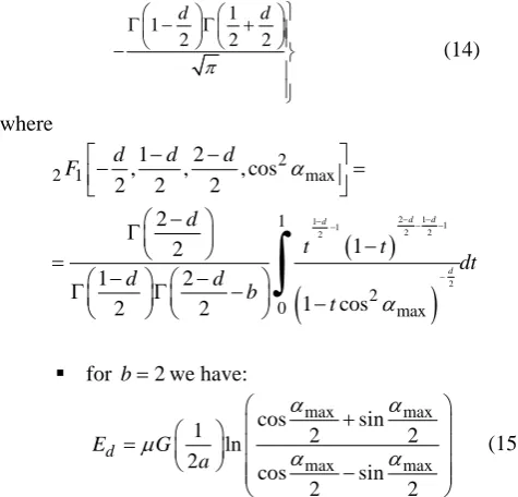
for b2we have:
max max
max max
cos sin
1 2 2
ln 2 cos sin 2 2 d E G a (15)
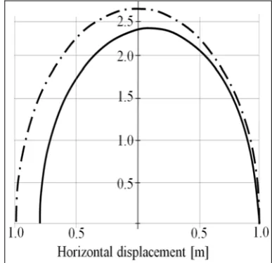
[image:3.595.305.543.52.280.2]In Fig. 4 we have represented the dissipated energies for the different sliding surfaces generated by the curves represented in Fig. 3. One can observe that for higher values of u there are significant changes in the dissipated energy for the analysed cases.
Fig. 4. The dissipated energies for the different sliding surfaces The kinetic energy of the structure of mass m is given by 2 2 k mv E
where v is the velocity. We denote by
max
p
E the maximum potential energy, given by:
max max
p
E mgh
So, if friction is not considered
max
k p p
E E E (16) 2 max 2 mv mgh mgh
and thus the maximum velocity, attended for u0 is
max
2
Fig. 5. The evolution of velocities and the heights
In Fig. 5 we have presented the evolution of velocities and the heights while the structure moves from the point of maximum vertical displacement to point O ( with u0), for different types of sliding surfaces generated by
2 0, 242
y u (with dashed line), y0, 275u2,5 (with solid line), y0,18u4 (with dash-dot line) and a circular arc with the radius R5(with dotted line).
If we consider friction, the velocity in point O is given by
max
2
2 Ed
v g h h
m
(18)
where Ed is the dissipated energy due to friction when the structure slides from point A to point O (see Fig. 2).
In the next pictures (Fig. 6, Fig. 7, Fig. 8 and Fig. 9) we have presented the evolution of velocities, first for the sliding without friction (with dash-dot line), next for the sliding with energy dissipation due to friction (with solid line), for the sliding surfaces generated by a circular arc with the radius R5 (Fig. 6), y0, 275u2,5 (Fig. 7),
2 0, 242
y u (Fig. 8) and for y0,18u4 (Fig. 9). Note that due to friction the structure no longer climbs to the same height it would climb if it were frictionless.
[image:4.595.329.533.49.230.2]Fig. 6. The evolution of velocities for the circular sliding surface, for the sliding with and without friction
Fig. 7. The evolution of velocities for the sliding surface generated by 2,5
0, 275
[image:4.595.332.526.279.466.2]y u , for the sliding with and without friction
Fig. 8. The evolution of velocities for the sliding surface generated by 2
0, 242
y u , for the sliding with and without friction
Fig. 9. The evolution of velocities for the sliding surface generated by 4
0,18
[image:4.595.333.536.526.690.2] [image:4.595.66.270.541.704.2]III. FINITE ELEMENT STUDY AND RESULTS
Earthquake isolation systems are devices located at the base of overhead structures, which have the aim to reduce the structure oscillating period during an earthquake and decrease the transmitted energy using frictional dissipation.
Classical isolation systems, with cylindrical or spherical sliding surfaces have the parts made of stainless steel, which provides durability. During earthquake, the slider and the concave surface of the lower plate maintain contact and consequently a relative uniform stress distribution is assured. For other types of sliding surfaces, limited contact occurs.
To prevent this kind of inconvenience, namely to obtain a continuum contact between the slider and the concave plate, it is necessary to insert an elastomeric layer between the slider and the sole, as presented in Fig. 10. This layer is similar to that used in elastomeric base isolation systems, assuring high portability [9]. So we can avoid incomplete contact (spotted or linear) and obtaining a controlled deformation for fit the concave shape of stationary plate.
Fig. 10. Friction pendulum with polynomial generated surface
The finite element analysis was made taking into account the real-scale model of an earthquake isolation system and transposing the whole loads, contacts and supports to virtual model using advanced nonlinear analysis software.
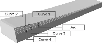
[image:5.595.76.275.576.661.2]Five curvature cases were analysed, one cylindrical and four based on surfaces generated by polynomials, like that presented in Fig. 11.
Fig. 11. Different types of sliding surfaces
For all cases, during the first second a vertical increasing load was applied, until it reaches the weight of superstructure. Afterwards, until the end of the considered time interval of 2 seconds, a predetermined course (simulating horizontal oscillation during an earthquake) was imposed.
TABLE II
Case Pressure max. [MPa]
Contact pressure shape 2[s] (sole)
Arc 0.55427
Curve 1 0.22301
Curve 2 0.22059
Curve 3 0.21550
Curve 4 0.21313
Three main types of contacts were used for seismic isolation system components: frictionless contact between first concave plate and slider, frictional contact (µ=0.15) between second concave plate and sole, bounded contact between elastomeric layer and sole, elastomeric layer and slider respectively.
Immediately after applying the vertical load, the sole is elastically deformed and in the contact area a contact patch is formed due to the pressure exerted by the elastomeric layer on the opposite side. This patch can be quantitatively evaluated using the contact pressure parameter. After 2 seconds, during the time period in which the horizontal displacement is imposed because the gliding assembly has been displaced, the contact patch becomes irregular with a slight increase of the pressure value in the rear of the sole, as we can see in Table II.
The normal stress distribution for entire assembly together with its maximum value, at the end of the analysed period, is presented in the Table III.
TABLE III Case Stress
max.[MP]
Normal stress 2[s] (Assembly)
Curve 1 0.21997
Curve 2 0.20032
Arc 0.19300
Curve 3 0.17180
Curve 4 0.17413
Curve 2 0.20032
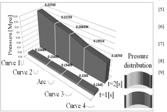
Fig. 12. Contact pressure between the upper concave plate and the slider determined after 1 and 2 seconds respectively
This diagram was obtained evaluating the contact region between upper concave plate and slider after the first time interval of 1[s] when the load is vertical and pressing the assembly and then at the end of the second time interval of 2[s] when the load is combined (horizontal and vertical).
IV. CONCLUSION
For classical earthquake isolation systems the dynamic response control is limited due to the reduced number of control parameters. In order to avoid this deficiency, this study shows the optimal way to improve the adjustment of elastic characteristics for a large exciter frequency spectrum of the earthquake.
The use of plates with concave surfaces generated by polynomials, for the case of friction, ensures higher speed near the equilibrium position, thus better conditions to restore the position prior to the earthquake.
Profile curves generated by polynomial functions show the possibilities to achieve the goal of superior, controlled energy dissipation.
While for the spherical surface the slider has the same shape with the concavity of the plate, for the sliding surfaces generated by other curves we must interpose, between the slider and lower armature, an elastomeric element able to follow the changes of the curvature. Finite element analysis proved that the normal stress values are reduced in case of use this kind of earthquake isolation system; all values for stress magnitude fall in the allowable range.
REFERENCES
[1] T. Hyakuda , K. Saito, T. Matsushita, N. Tanaka, S. Yoneki, M. Yasuda, M. Miyazaki, A. Suzuki, T. Sawada, The structural design and earthquake observation of a seismic isolation building using Friction Pendulum system, Proceedings, 7th International Seminar on Seismic Isolation, Passive Energy Dissipation and Active Control of Vibrations of Structures, Assisi, Italy, 2001.
[2] Y. B. Yang, T. Y. Lee and I. C. Tsai, Response of multi-degree-of- freedom structure with sliding supports, Earthquake Engrg. Struct. Dyn. 19, 739Ð752 , 1990.
[3] P. Roussis , M.C. Constantinou , Uplift-restraining friction pendulum seismic isolation system, Earthq. Eng. Struct. Dyn. 35:577–593, 2006.
[4] V.A. Zayas, S.S. Low, S.A. Mahin, A simple pendulum technique for achieving seismic isolation, Earthquake Spectra 6, 317-333, 1990. [5] MC. Constantinou, Friction Pendulum double concave bearing.
NEES Report, available at: http://nees.buffalo.edu/docs/dec304/FP - DC%20Report-DEMO.pdf, 2004.
[6] CS. Tsai, TC. Chiang, BJ. Chen., Finite element formulations and theoretical study for variable curvature friction pendulum system , Engineering Structures 25, 2003, 1719-1730.
[7] M. Pranesh, R. Sinha, Aseismic design of structure-equipament systems using variable frequency pendulum isolator, Nuclear Engineering and Design 231, 2004, 129-139.
[8] M. Pranesh, R. Sinha, VFPI: an isolation device for aseismic design, Earthquake Engn. Struct. Dyn. 2000, 29, 603-627.