An Exploration of Word Embedding Initialization in Deep Learning Tasks

S Bandyopadhyay, D S Sharma and R Sangal. Proc. of the 14th Intl. Conference on Natural Language Processing, pages 56–64, Kolkata, India. December 2017. c2016 NLP Association of India (NLPAI)

An Exploration of Word Embedding Initialization

in Deep-Learning Tasks

Tom Kocmi and Ondˇrej Bojar Charles University,

Faculty of Mathematics and Physics Institute of Formal and Applied Linguistics

[email protected]

Abstract

Word embeddings are the interface be-tween the world of discrete units of text processing and the continuous, differen-tiable world of neural networks. In this work, we examine various random and pretrained initialization methods for em-beddings used in deep networks and their effect on the performance on four NLP tasks with both recurrent and convolu-tional architectures. We confirm that pre-trained embeddings are a little better than random initialization, especially consider-ing the speed of learnconsider-ing. On the other hand, we do not see any significant dif-ference between various methods of ran-dom initialization, as long as the variance is kept reasonably low. High-variance ini-tialization prevents the network to use the space of embeddings and forces it to use other free parameters to accomplish the task. We support this hypothesis by ob-serving the performance in learning lexical relations and by the fact that the network can learn to perform reasonably in its task even with fixed random embeddings.

1 Introduction

Embeddings or lookup tables (Bengio et al., 2003) are used for units of different granularity, from characters (Lee et al., 2016) to subword units (Sennrich et al., 2016; Wu et al., 2016) up to words. In this paper, we focus solely on word embeddings (embeddings attached to individual token types in the text). In their highly dimen-sional vector space, word embeddings are capa-ble of representing many aspects of similarities be-tween words: semantic relations or morphological properties (Mikolov et al., 2013; Kocmi and Bojar,

2016) in one language or cross-lingually (Luong et al., 2015).

Embeddings are trained for a task. In other words, the vectors that embeddings assign to each word type are almost never provided manually but always discovered automatically in a neural net-work trained to carry out a particular task. The well known embeddings are those by Mikolov et al. (2013), where the task is to predict the word from its neighboring words (CBOW) or the neigh-bors from the given word (Skip-gram). Trained on a huge corpus, these “Word2Vec” embeddings show an interesting correspondence between lexi-cal relations and arithmetic operations in the vec-tor space. The most famous example is the follow-ing:

v(king)₋v(man) +v(woman)_≈v(queen)

In other words, adding the vectors associated with the words ‘king’ and ‘woman’ while subtracting ‘man’ should be equal to the vector associated with the word ‘queen’. We can also say that the difference vectors v(king) ₋ v(queen) and

v(man)−v(woman)are almost identical and

de-scribe the gender relationship.

Word2Vec is not trained with a goal of proper representation of relationships, therefore the ab-solute accuracy scores around 50% do not allow to rely on these relation predictions. Still, it is a rather interesting property observed empirically in the learned space. Another extensive study of em-bedding space has been conducted by Hill et al. (2017).

dataset1 _{and GloVe embeddings were trained on}

6 billion words from the Wikipedia. Sometimes, they are used as a fixed mapping for a better robustness of the system (Kenter and De Rijke, 2015), but they are more often used to seed the em-beddings in a system and they are further trained in the particular end-to-end application (Collobert et al., 2011; Lample et al., 2016).

In practice, random initialization of embeddings is still more common than using pretrained embed-dings and it should be noted that pretrained em-beddings are not always better than random ini-tialization (Dhingra et al., 2017).

We are not aware of any study of the effects of various random embeddings initializations on the training performance.

In the first part of the paper, we explore various English word embeddings initializations in four tasks: neural machine translation (denotedMT in the following for short), language modeling (LM), part-of-speech tagging (TAG) and lemmatization (LEM), covering both common styles of neural ar-chitectures: the recurrent and convolutional neural networks, RNN and CNN, resp.

In the second part, we explore the obtained em-beddings spaces in an attempt to better understand the networks have learned about word relations.

2 Embeddings initialization

Given a vocabularyV of words, embeddings

rep-resent each word as a dense vector of sized (as

opposed to “one-hot” representation where each word would be represented as a sparse vector of size|V_|with all zeros except for one element

in-dicating the given word). Formally, embeddings are stored in a matrixE_∈R|V|×d.

For a given word type w ∈ V, a row is

se-lected from E. Thus, E is often referred to as

word lookup table. The size of embeddingsdis often set between 100 and 1000 (Bahdanau et al., 2014; Vaswani et al., 2017; Gehring et al., 2017).

2.1 Initialization methods

Many different methods can be used to initialize the values inEat the beginning of neural network

training. We distinguish between randomly initial-ized and pretrained embeddings, where the latter can be further divided into embeddings pretrained

1_{See https://code.google.com/archive/p/}

word2vec/.

on the same task and pretrained on a standard task such as Word2Vec or GloVe.

Random initialization methods common in the literature2 _{sample values either uniformly from a}

fixed interval centered at zero or, more often, from a zero-mean normal distribution with the standard deviation varying from 0.001 to 10.

The parameters of the distribution can be set empirically or calculated based on some assump-tions about the training of the network. The sec-ond approach has been done for various hidden layer initializations (i.e. not the embedding layer). E.g. Glorot and Bengio (2010) and He et al. (2015) argue that sustaining variance of values thorough the whole network leads to the best results and define the parameters for initialization so that the layer weightsW have the same variance of output

as is the variance of the input.

Glorot and Bengio (2010) define the “Xavier” initialization method. They suppose a linear neu-ral network for which they derive weights initial-ization as

W ∼ U− √

6 √

ni+no

; √

6 √

ni+no

(1)

whereniis the size of the input andnois the size

of the output. The initialization for nonlinear net-works using ReLu units has been derived similarly by He et al. (2015) as

W _{∼ N}(0, 2 ni

) (2)

The same assumption of sustaining variance can-not be applied to embeddings because there is no input signal whose variance should be sustained to the output. We nevertheless try these initializa-tion as well, denoting themXavierandHe, respec-tively.

2.2 Pretrained embeddings

Pretrained embeddings, as opposed to random ini-tialization, could work better, because they already contain some information about word relations.

on the same task. Such embeddings contain infor-mation useful for the task in question and we refer to them asself-pretrain.

A more common approach is to download some ready-made “generic” embeddings such as Word2Vec and GloVe, whose are not directly related to the final task but show to contain many morpho-syntactic relations between words (Mikolov et al., 2013; Kocmi and Bojar, 2016). Those embeddings are trained on billions of monolingual examples and can be easily reused in most existing neural architectures.

3 Experimental setup

This section describes the neural models we use for our four tasks and the training and testing datasets.

3.1 Models description

For all our four tasks (MT, LM, TAG, and LEM), we use Neural Monkey (Helcl and Libovick´y, 2017), an open-source neural machine translation and general sequence-to-sequence learning system built using the TensorFlow machine learning li-brary.

All models use the same vocabulary of 50000 most frequent words from the training corpus. And the size of embedding is set to 300, to match the dimensionality of the available pre-trained Word2Vec and GloVe embeddings.

All tasks are trained using the Adam (Kingma and Ba, 2014) optimization algorithm.

We are using 4GB machine translation setup (MT) as described in Bojar et al. (2017) with in-creased encoder and decoder RNN sizes. The setup is the encoder-decoder architecture with at-tention mechanism as proposed by Bahdanau et al. (2014). We use encoder RNN with 500 GRU cells for each direction (forward and backward), decoder RNN with 450 conditional GRU cells, maximal length of 50 words and no dropout. We evaluate the performance using BLEU (Papineni et al., 2002). Because our aim is not to surpass the state-of-the-artMTperformance, we omit com-mon extensions like beam search or ensembling. Pretrained embeddings also prevent us from using subword units (Sennrich et al., 2016) or a larger embedding size, as customary in NMT. We exper-iment only with English-to-Czech MT and when using pretrained embeddings we modify only the source-side (encoder) embeddings, because there

are no pretrained embeddings available for Czech. The goal of the language model (LM) is to pre-dict the next word based on the history of previous words. Language modeling can be thus seen as (neural) machine translation without the encoder part: no source sentence is given to translate and we only predict words conditioned on the previ-ous word and the state computed from predicted words. Therefore the parameters of the neural net-work are the same as for theMTdecoder. The only difference is that we use dropout with keep prob-ability of 0.7 (Srivastava et al., 2014). The gener-ated sentence is evalugener-ated as the perplexity against the gold output words (English in our case).

The third task is the POS tagging (TAG). We use our custom network architecture: The model starts with a bidirectional encoder as in MT. For each encoder state, a fully connected linear layer then predicts a tag. The parameters are set to be equal to the encoder in MT, the predicting layer have a size equal to the number of tags. TAG is evaluated by the accuracy of predicting the correct POS tag.

The last task examined in this paper is the lemmatization of words in a given sentence (LEM). For this task we have decided to use the convolu-tional neural network, which is second most used architecture in neural language processing next to the recurrent neural networks. We use the con-volutional encoder as defined by Gehring et al. (2017) and for each state of the encoder, we pre-dict the lemma with a fully connected linear layer. The parameters are identical to the cited work. LEM is evaluated by a accuracy of predicting the correct lemma.

When using pretrained Word2Vec and GloVe embeddings, we face the problem of different vo-cabularies not compatible with ours. Therefore for words in our vocabulary not covered by the pre-trained embeddings, we sample the embeddings from the zero-mean normal distribution with a standard deviation of0.01.

3.2 Training and testing datasets

We use CzEng 1.6 (Bojar et al., 2016), a parallel Czech-English corpus containing over 62.5 mil-lion sentence pairs. This dataset already contains automatic word lemmas and POS tags.3

Initialization MTen-cs (25M) LM(25M) RNNTAG(3M) CNNLEM(3M)

N(0,10) 6.93 BLEU 76.95 85.2 % 48.4 %

N(0,1) 9.81 BLEU 61.36 87.9 % 94.4 %

N(0,0.1) 11.77 BLEU 56.61 90.7 % 95.7 %

N(0,0.01) 11.77 BLEU 56.37 90.8 % 95.9 %

N(0,0.001) 11.88 BLEU 55.66 90.5 % 95.9 %

Zeros 11.65 BLEU 56.34 90.7 % 95.9 %

Ones 10.63 BLEU 62.04 90.2 % 95.7 %

He init. 11.74 BLEU 56.40 90.7 % 95.7 %

Xavier init. 11.67 BLEU 55.95 90.8 % 95.9 %

Word2Vec 12.37 BLEU 54.43 90.9 % 95.7 %

Word2Vec on trainset 11.74 BLEU 54.63 90.8 % 95.6 %

GloVe 11.90 BLEU 55.56 90.6 % 95.5 %

Self pretrain 12.61 BLEU 54.56 91.1 % 95.9 %

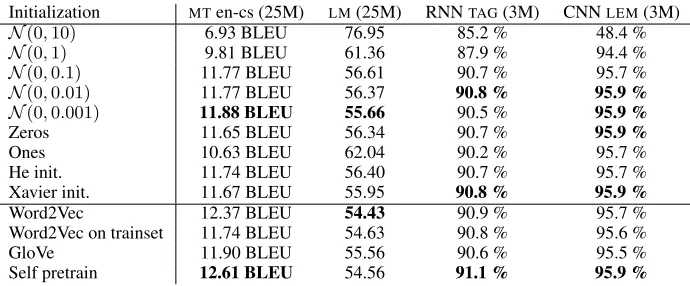
Table 1: Task performance with various embedding initializations. Except forLM, higher is better. The best results for random (upper part) and pretrained (lower part) embedding initializations are in bold.

We use the newstest2016 dataset from WMT 20164 _{as the testset for MT, LM andLEM.}

The size of the testset is 2999 sentence pairs con-taining 57 thousands Czech and 67 thousands En-glish running words.

For TAG, we use manually annotated English tags from PCEDT5 _{(Hajiˇc et al., 2012). From}

this dataset, we drop all sentences containing the tag “-NONE-” which is not part of the standard tags. This leads to the testset of 13060 sentences of 228k running words.

4 Experiments

In this section, we experimentally evaluate em-bedding initialization methods across four differ-ent tasks and two architectures: the recurrdiffer-ent and convolutional neural networks.

The experiments are performed on the NVidia GeForce 1080 graphic card. Note that each run of MT takes a week of training, LM takes a day and a half andTAGandLEM need several hours each. We run the training for one epoch and evaluate the performance regularly throughout the training on the described test set. ForMT andLM, the epoch amounts to 25M sentence pairs and forTAG and LEM to 3M sentences. The epoch size is set em-pirically so that the models already reach a sta-ble level of performance and further improvement does not increase the performance too much.

MT and LM exhibit performance fluctuation throughout the training. Therefore, we average the results over five consecutive evaluation scores

that this difference will have no effect on the comparison of embeddings initializations and we prefer to use the same training dataset for all our tasks.

4_{http://www.statmt.org/wmt16/translation-task.html} 5_{https://ufal.mff.cuni.cz/pcedt2.0/en/index.html}

spread across 500k training examples to avoid lo-cal fluctuations. This can be seen as a simple smoothing method.6

4.1 Final performance

In this section, we compare various initialization methods based on the final performance reached in the individual tasks. Intuitively, one would ex-pect the best performance with self-pretrained em-beddings, followed by Word2Vec and GloVe. The random embeddings should perform worse.

Table 1 shows the influence of the embedding initialization on various tasks and architectures.

The rowsonesandzerosspecify the

initializa-tion with a single fixed value.

The “Word2Vec on trainset” are pretrained em-beddings which we created by running Gensim ( ˇReh˚uˇrek and Sojka, 2010) on our training set. This setup serves as a baseline for the embeddings pretrained on huge monolingual corpora and we can notice a small loss in performance compared to both Word2Vec and GloVe.

We can notice several interesting results. As expected, the self-pretrained embeddings slightly outperform pretrained Word2Vec and GloVe, which are generally slightly better than random initializations.

A more important finding is that there is gen-erally no significant difference in the performance between different random initialization methods, exceptonesand setups with the standard deviation

of 1 and higher, all of which perform considerably worse.

6_{See, e.g. http://www.itl.nist.gov/div898/}

handbook/pmc/section4/pmc42.htmfrom Natrella

(2010) justifying the use of the simple average, provided that the series has leveled off, which holds in our case.

50 55 60 65 70 75 80 85 90 95 100

0 5 10 15 20 25

Perple

xity

Steps (in millions examples)

Normal std=10 Normal std=1 Ones Remaining methods Word2Vec Selftrain

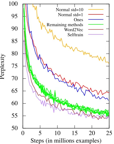
Figure 1: Learning curves for language model-ing. The testing perplexity is computed every 300k training examples. Label ”Remaining meth-ods” represents all learning curves for the methods from Table 1 not mentioned otherwise.

Any random initialization with standard devia-tion smaller than 0.1 leads to similar results, in-cluding even thezeroinitialization.7 We attempt

to explain this behavior in Section 5.

4.2 Learning speed

While we saw in Table 1 that most of the initial-ization methods lead to a similar performance, the course of the learning is slightly more varied. In other words, different initializations need different numbers of training steps to arrive at a particular performance. This is illustrated in Figure 1 forLM. To describe the situation concisely across the tasks, we set a minimal score for each task and we measure how many examples did the training need to reach the score. We set the scores as follows: MT needs to reach 10 BLEU points, LM needs to reach the perplexity of 60,TAGneeds to reach the accuracy of 90% andLEM needs to reach the ac-curacy of 94%.

We use a smoothing window as implemented in TensorBoard with a weight of 0.6 to smooth the 7_{It could be seen as a surprise, that zero initialization} works at all. But since embeddings behave as weights for bias values, they learn quickly from the random weights available throughout the network.

Initialization MTen-cs LM TAG LEM N(0,1) 25.3M 37.3M 10.6M 2.7M

N(0,0.1) 9.7M 13.5M 2.0M 1.8M

N(0,0.01) 9.8M 12.0M 1.4M 1.2M

N(0,0.001) 9.8M 12.0M 1.0M 0.5M

Zeros 9.4M 12.3M 1.0M 0.5M

Ones 18.9M 26.7M 2.9M 0.8M

He init. 9.5M 12.5M 1.0M 0.5M

Xavier init. 9.2M 12.3M 1.0M 0.5M

Word2Vec 6.9M 7.9M 0.7M 1.2M

GloVe 8.6M 11.4M 1.9M 1.3M

Self pretrain 5.2M 5.7M 0.2M 0.9M

Table 2: The number of training examples needed to reach a desired score.

testing results throughout the learning. This way, we avoid small fluctuations in training and our es-timate when the desired value was reached is more reliable.

The results are in Table 2. We can notice that pretrained embeddings converge faster than the randomly initialized ones on recurrent architecture (MT,LMandTAG) but not on the convolutional ar-chitecture (LEM).

Self-pretrained embeddings are generally much better. Word2Vec also performs very well but GloVe embeddings are worse than random initial-izations forTAG.

5 Exploration of embeddings space

We saw above that pretrained embeddings are slightly better than random initialization. We also saw that the differences in performance are not significant when initialized randomly with small values.

In this section, we analyze how specific lex-ical relations between words are represented in the learned embeddings space. Moreover, based on the observations from the previous section, we propose a hypothesis about the failure of initial-ization with big numbers (ones or high-variance random initialization) and try to justify it.

The hypothesis is as follows:

ral network free choice over the utilization of the embedding space.

We support our hypothesis as follows.

• We examine the embedding space on the per-formance in lexical relations between words, If our hypothesis is plausible, low-variance embeddings will perform better at represent-ing these relations.

• We run an experiment with non-trainable fixed random initialization to demonstrate the ability of the neural network to overcome broken embeddings and to learn the informa-tion about words in its deeper hidden layers.

5.1 Lexical relations

Recent work on word embeddings (Vylomova et al., 2016; Mikolov et al., 2013) has shown that simple vector operations over the embeddings are surprisingly effective at capturing various seman-tic and morphosyntacseman-tic relations, despite lacking explicit supervision in these respects.

The testset by Mikolov et al. (2013) contains “questions” defined as v(X)₋v(Y) +v(A) _∼

v(B). The well-known example involves

predict-ing a vector for word ‘queen’ from the vector com-bination ofv(king)₋v(man) +v(woman). This

example is a part of “semantic relations” in the test set, called opposite-gender. The dataset contain another 4 semantic relations and 9 morphosyn-tactic relations such as pluralisation v(cars) ₋

v(car) +v(apple)∼v(apples).

Kocmi and Bojar (2016) revealed the sparsity of the testset and presented extended testset. Both testsets are compatible and we use them in combi-nation.

Note that the performance on this test set is af-fected by the vocabulary overlap between the test set and the vocabulary of the embeddings; ques-tions containing out-of-vocabulary words cannot be evaluated. This is the main reason, why we trained all tasks on the same training set and with the same vocabulary, so that their performance in lexical relations can be directly compared.

Another lexical relation benchmark is the word similarity. The idea is that similar words such as ‘football’ and ‘soccer’ should have vectors close together. There exist many datasets dealing with word similarity. Faruqui and Dyer (2014) have extracted words similarity pairs from 12 different

Initialization MTen-cs LM LEM

N(0,10) 0.0; 0.3 0.0; 0.3 0.0; 0.3 N(0,1) 0.0; 0.4 1.4; 3.5 0.0; 0.3 N(0,0.1) 1.2; 23.5 5.5; 15.2 0.0; 0.8 N(0,0.01) 2.0; 29.9 6.9; 19.4 0.1; 32.7 N(0,0.001) 2.1; 31.4 6.7; 18.2 0.3; 33.3 Zeros 1.6; 29.5 6.0; 17.5 0.2; 31.1 Ones 0.5; 16.6 5.3; 9.3 0.1; 31.0 He init. 1.4; 28.9 7.7; 18.3 0.1; 32.6 Xavier init. 1.5; 29.5 7.4; 18.2 0.1; 32.7 Word2Vec on trainset* 22.3; 48.9

Word2Vec official* 81.3; 70.7 GloVe official* 12.3; 60.1

Table 3: The accuracy in percent on the (seman-tic; morphosyntactic) questions. We do not re-port TAG since its accuracy was less than 1% on all questions. *For comparison, we present results of Word2Vec trained on our training set and offi-cial trained embeddings before applying them on training of particular task.

Initialization MTen-cs LM TAG LEM

N(0,10) 3.3 2.2 3.6 2.6

N(0,1) 15.7 11.8 3.5 2.7

N(0,0.1) 56.7 32.7 6.9 2.8

N(0,0.01) 62.5 41.0 12.8 4.7

N(0,0.001) 59.3 37.4 12.1 2.4

Zeros 57.9 37.4 12.8 3.5

Ones 34.0 19.3 11.4 4.3

He init. 58.2 37.4 12.3 4.2 Xavier init. 58.3 37.5 12.3 2.7

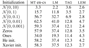
Table 4: Spearman’s correlation ρ on word

simi-larities. The results are multiplied by 100.

corpora and created an interface for testing the em-beddings on the word similarity task.8

When evaluating the task, we calculate the sim-ilarity between a given pair of words by the co-sine similarity between their corresponding vector representation. We then report Spearmans rank correlation coefficient between the rankings pro-duced by the embeddings against human rank-ings. For convenience, we combine absolute val-ues of Spearman’s correlations from all 12 Faruqui and Dyer (2014) testsets together as an average weighted by the number of words in the datasets.

The last type of relation we examine are the nearest neighbors. We illustrate on the TAGtask how the embedding space is clustered when vari-ous initializations are used. We employ the Prin-cipal component analysis (PCA) to convert the embedding space of |E| dimensions into two-dimensional space.

Table 3 reflects several interesting properties 8_{http://wordvectors.org/}

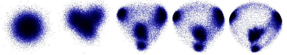
Figure 2: A representation of words in the trained embeddings forTAGtask projected by PCA. From left to right it shows trained embeddings forN(0,1),N(0,0.1),N(0,0.01),N(0,0.001)andzeros. Note

that except of the first model all of them reached a similar performance on theTAGtask.

about the embedding space. We see task-specific behavior, e.g. TAG not learning any of the tested relationships whatsoever orLMbeing the only task that learned at least something of semantic rela-tions.

The most interesting property is that when in-creasing the variance of initial embedding, the performance dramatically drops after some point. LEM reveals this behavior the most: the network initialized by normal distribution with standard deviation of 0.1 does not learn any relations but still performs comparably with other initialization methods as presented in Table 1. We ran the lemmatization experiments once again in order to confirm that it is not only a training fluctuation.

This behavior suggests that the neural network can work around broken embeddings and learn im-portant features within other hidden layers instead of embeddings.

A similar behavior can be traced also in the word similarity evaluation in Table 4, where mod-els are able to learn to solve their tasks and still not learn any information about word similarities in the embeddings.

Finally, when comparing the embedded space of embeddings as trained byTAGin Figure 2, we see a similar behavior. With lower variance in embeddings initialization, the learned embeddings are more clearly separated.

This suggests that when the neural network has enough freedom over the embeddings space, it uses it to store information about the relations be-tween words.

5.2 Non-trainable embeddings

To conclude our hypothesis, we demonstrate the flexibility of a neural network to learn despite a broken embedding layer.

In this experiment, the embeddings are fixed

Initialization MTen-cs LM TAG LEM N(0,10) 7.28 BLEU 79.44 47.3 % 85.5 % N(0,1) 8.46 BLEU 78.68 87.1 % 94.0 % N(0,0.01) 6.84 BLEU 82.84 63.2 % 91.1 % Word2Vec 8.71 BLEU 60.23 88.4 % 94.1 %

Table 5: The results of the experiment when learned with non-trainable embeddings.

and the neural network cannot modify them during the training process. Therefore, it needs to find a way to learn the representation of words in other hidden layers.

As in Section 4.1, we train models for 3M ex-amples forTAGandLEMand for over 25M exam-ples forMTandLM.

Table 5 confirms that the neural network is flex-ible enough to partly overcome the problem with fixed embeddings. For example, MT initialized withN(0,1)reaches the score of 8.46 BLEU with fixed embeddings compared to 9.81 BLEU for the same but not fixed (trainable) embeddings.

When embeddings are fixed at random values, the effect is very similar to embeddings with high-variance random initialization. The network can distinguish the words through the crippled embed-dings but has no way to improve them. It thus pro-ceeds to learn in a similar fashion as with one-hot representation.

6 Conclusion

In this paper, we compared several initializa-tion methods of embeddings on four different tasks, namely: machine translation (RNN), lan-guage modeling (RNN), POS tagging (RNN) and lemmatization (CNN).

The experiments indicate that pretrained em-beddings converge faster than random initializa-tion and that they reach a slightly better final per-formance.

The examined random initialization methods do not lead to significant differences in the perfor-mance as long as the initialization is within rea-sonable variance (i.e. standard deviation smaller than0.1). Higher variance apparently prevents the

network to adapt the embeddings to its needs and the network resorts to learning in its other free pa-rameters. We support this explanation by showing that the network is flexible enough to overcome even non-trainable embeddings.

We also showed a somewhat unintuitive result that when the neural network is presented with em-beddings with a small variance or even all-zeros embeddings, it utilizes the space and learns (to some extent) relations between words in a way similar to Word2Vec learning.

Acknowledgement

This work has been in part supported by the European Union’s Horizon 2020 research and innovation programme under grant agreements No 644402 (HimL) and 645452 (QT21), by the LINDAT/CLARIN project of the Ministry of Education, Youth and Sports of the Czech Republic (projects LM2015071 and OP VVV VI CZ.02.1.01/0.0/0.0/16 013/0001781), by the Charles University Research Programme “Pro-gres” Q18+Q48, by the Charles University SVV project number 260 453 and by the grant GAUK 8502/2016.

References

Dzmitry Bahdanau, Kyunghyun Cho, and Yoshua Ben-gio. 2014. Neural machine translation by jointly learning to align and translate. InICLR 2015.

Yoshua Bengio, R´ejean Ducharme, Pascal Vincent, and Christian Jauvin. 2003. A neural probabilistic lan-guage model.Journal of machine learning research, 3(Feb):1137–1155.

Ondˇrej Bojar, Ondˇrej Duˇsek, Tom Kocmi, Jindˇrich Li-bovick´y, Michal Nov´ak, Martin Popel, Roman Su-darikov, and Duˇsan Variˇs. 2016. Czeng 1.6: En-larged czech-english parallel corpus with process-ing tools dockered. In Petr Sojka, Aleˇs Hor´ak, Ivan Kopeˇcek, and Karel Pala, editors,Text, Speech, and Dialogue: 19th International Conference, TSD 2016, number 9924 in Lecture Notes in Com-puter Science, pages 231–238. Masaryk University, Springer International Publishing.

Ondˇrej Bojar, Jindˇrich Helcl, Tom Kocmi, Jindˇrich Li-bovick´y, and Tom´aˇs Musil. 2017. Results of the

WMT17 Neural MT Training Task. In Proceed-ings of the 2nd Conference on Machine Translation (WMT), Copenhagen, Denmark, September.

Ronan Collobert, Jason Weston, L´eon Bottou, Michael Karlen, Koray Kavukcuoglu, and Pavel Kuksa. 2011. Natural language processing (almost) from scratch. Journal of Machine Learning Research, 12(Aug):2493–2537.

Bhuwan Dhingra, Hanxiao Liu, Ruslan Salakhutdinov, and William W. Cohen. 2017. A comparative study of word embeddings for reading comprehen-sion.CoRR, abs/1703.00993.

Manaal Faruqui and Chris Dyer. 2014. Community evaluation and exchange of word vectors at word-vectors.org. InProceedings of ACL: System Demon-strations.

Jonas Gehring, Michael Auli, David Grangier, Denis Yarats, and Yann Dauphin. 2017. Convolutional se-quence to sese-quence learning.

Xavier Glorot and Yoshua Bengio. 2010. Understand-ing the difficulty of trainUnderstand-ing deep feedforward neu-ral networks. InProceedings of the Thirteenth In-ternational Conference on Artificial Intelligence and Statistics, pages 249–256.

Jan Hajiˇc, Eva Hajiˇcov´a, Jarmila Panevov´a, Petr Sgall, Ondˇrej Bojar, Silvie Cinkov´a, Eva Fuˇc´ıkov´a, Marie Mikulov´a, Petr Pajas, Jan Popelka, Jiˇr´ı Semeck´y, Jana ˇSindlerov´a, Jan ˇStˇep´anek, Josef Toman, Zdeˇnka Ureˇsov´a, and Zdenˇek ˇZabokrtsk´y. 2012. Announcing Prague Czech-English Depen-dency Treebank 2.0. InProceedings of the Eighth International Language Resources and Evaluation Conference (LREC’12), pages 3153–3160, Istanbul, Turkey, May. ELRA, European Language Resources Association.

Kaiming He, Xiangyu Zhang, Shaoqing Ren, and Jian Sun. 2015. Delving deep into rectifiers: Surpass-ing human-level performance on imagenet classifi-cation. In Proceedings of the IEEE international conference on computer vision, pages 1026–1034.

Jindˇrich Helcl and Jindˇrich Libovick´y. 2017. Neural monkey: An open-source tool for sequence learn-ing. The Prague Bulletin of Mathematical Linguis-tics, 107:5–17.

Felix Hill, Kyunghyun Cho, S´ebastien Jean, and Yoshua Bengio. 2017. The representational geom-etry of word meanings acquired by neural machine translation models. Machine Translation, pages 1– 16.

Tom Kenter and Maarten De Rijke. 2015. Short text similarity with word embeddings. InProceedings of the 24th ACM International on Conference on Infor-mation and Knowledge Management, pages 1411– 1420. ACM.

Diederik P. Kingma and Jimmy Ba. 2014. Adam: A method for stochastic optimization. CoRR, abs/1412.6980.

Tom Kocmi and Ondˇrej Bojar, 2016. SubGram: Ex-tending Skip-Gram Word Representation with Sub-strings, pages 182–189. Springer International Pub-lishing.

Guillaume Lample, Miguel Ballesteros, Kazuya Kawakami, Sandeep Subramanian, and Chris Dyer. 2016. Neural architectures for named entity recog-nition. InIn proceedings of NAACL-HLT (NAACL 2016)., San Diego, US.

Jason Lee, Kyunghyun Cho, and Thomas Hof-mann. 2016. Fully character-level neural machine translation without explicit segmentation. CoRR, abs/1610.03017.

Minh-Thang Luong, Hieu Pham, and Christopher D. Manning. 2015. Bilingual word representations with monolingual quality in mind. InNAACL Work-shop on Vector Space Modeling for NLP, Denver, United States.

Tomas Mikolov, Kai Chen, Greg Corrado, and Jeffrey Dean. 2013. Efficient estimation of word represen-tations in vector space.CoRR, abs/1301.3781.

Mary Natrella. 2010. Nist/sematech e-handbook of statistical methods.

Kishore Papineni, Salim Roukos, Todd Ward, and Wei-Jing Zhu. 2002. BLEU: a Method for Automatic Evaluation of Machine Translation. InACL 2002, Proceedings of the 40th Annual Meeting of the As-sociation for Computational Linguistics, pages 311– 318, Philadelphia, Pennsylvania.

Jeffrey Pennington, Richard Socher, and Christo-pher D. Manning. 2014. Glove: Global vectors for word representation. InEmpirical Methods in Nat-ural Language Processing (EMNLP), pages 1532– 1543.

Radim ˇReh˚uˇrek and Petr Sojka. 2010. Software Framework for Topic Modelling with Large Cor-pora. InProceedings of the LREC 2010 Workshop on New Challenges for NLP Frameworks, pages 45– 50, Valletta, Malta, May. ELRA. http://is.

muni.cz/publication/884893/en.

Rico Sennrich, Barry Haddow, and Alexandra Birch. 2016. Neural machine translation of rare words with subword units. In Proceedings of the 54th Annual Meeting of the Association for Computa-tional Linguistics (Volume 1: Long Papers), pages 1715–1725, Berlin, Germany, August. Association for Computational Linguistics.

Nitish Srivastava, Geoffrey Hinton, Alex Krizhevsky, Ilya Sutskever, and Ruslan Salakhutdinov. 2014. Dropout: A simple way to prevent neural networks from overfitting. Journal of Machine Learning Re-search, 15:1929–1958.

A. Vaswani, N. Shazeer, N. Parmar, J. Uszkoreit, L. Jones, A. N. Gomez, L. Kaiser, and I. Polosukhin. 2017. Attention is all you need.ArXiv e-prints, jun.

Ekaterina Vylomova, Laura Rimell, Trevor Cohn, and Timothy Baldwin. 2016. Take and took, gaggle and goose, book and read: Evaluating the utility of vector differences for lexical relation learning. In

Proceedings of the 54th Annual Meeting of the As-sociation for Computational Linguistics (Volume 1: Long Papers), pages 1671–1682, Berlin, Germany, August. Association for Computational Linguistics.

Yonghui Wu, Mike Schuster, Zhifeng Chen, Quoc V Le, Mohammad Norouzi, Wolfgang Macherey, Maxim Krikun, Yuan Cao, Qin Gao, Klaus Macherey, et al. 2016. Google’s neural ma-chine translation system: Bridging the gap between human and machine translation. arXiv preprint arXiv:1609.08144.