Proceedings of NAACL-HLT 2018, pages 1470–1480
KBGAN
: Adversarial Learning for Knowledge Graph Embeddings
Liwei Cai
Department of Electronic Engineering Tsinghua University
Beijing 100084 China [email protected]
William Yang Wang
Department of Computer Science University of California, Santa Barbara
Santa Barbara, CA 93106 USA [email protected]
Abstract
We introduceKBGAN, an adversarial learning framework to improve the performances of a wide range of existing knowledge graph em-bedding models. Because knowledge graphs typically only contain positive facts, sampling useful negative training examples is a non-trivial task. Replacing the head or tail entity of a fact with a uniformly randomly selected entity is a conventional method for generat-ing negative facts, but the majority of the gen-erated negative facts can be easily discrimi-nated from positive facts, and will contribute little towards the training. Inspired by genera-tive adversarial networks (GANs), we use one knowledge graph embedding model as a neg-ative sample generator to assist the training of our desired model, which acts as the dis-criminator in GANs. This framework is inde-pendent of the concrete form of generator and discriminator, and therefore can utilize a wide variety of knowledge graph embedding mod-els as its building blocks. In experiments, we adversarially train two translation-based mod-els, TRANSE and TRANSD, each with assis-tance from one of the two probability-based models, DISTMULTand COMPLEX. We eval-uate the performances ofKBGAN on the link prediction task, using three knowledge base completion datasets: FB15k-237, WN18 and WN18RR. Experimental results show that ad-versarial training substantially improves the performances of target embedding models un-der various settings.
1 Introduction
Knowledge graph (Dong et al., 2014) is a pow-erful graph structure that can provide direct ac-cess of knowledge to users via various applica-tions such as structured search, question answer-ing, and intelligent virtual assistant. A common representation of knowledge graph beliefs is in the
form of a discrete relational triple such as Locate-dIn(NewOrleans,Louisiana).
A main challenge for using discrete represen-tation of knowledge graph is the lack of capa-bility of accessing the similarities among differ-ent differ-entities and relations. Knowledge graph em-bedding (KGE) techniques (e.g.,RESCAL(Nickel et al.,2011), TRANSE (Bordes et al.,2013), DIST -MULT(Yang et al.,2015), and COMPLEX (Trouil-lon et al., 2016)) have been proposed in recent years to deal with the issue. The main idea is to represent the entities and relations in a vec-tor space, and one can use machine learning tech-nique to learn the continuous representation of the knowledge graph in the latent space.
However, even steady progress has been made in developing novel algorithms for knowledge graph embedding, there is still a common chal-lenge in this line of research. For space effi-ciency, common knowledge graphs such as Free-base (Bollacker et al., 2008), Yago (Suchanek et al.,2007), and NELL (Mitchell et al.,2015) by default only stores beliefs, rather than disbeliefs. Therefore, when training the embedding models, there is only the natural presence of the positive examples. To use negative examples, a common method is to remove the correct tail entity, and ran-domly sample from a uniform distribution (Bordes et al., 2013). Unfortunately, this approach is not ideal, because the sampled entity could be com-pletely unrelated to the head and the target re-lation, and thus the quality of randomly gener-ated negative examples is often poor (e.g, Locate-dIn(NewOrleans,BarackObama)). Other approach might leverage external ontological constraints such as entity types (Krompaß et al.,2015) to gen-erate negative examples, but such resource does not always exist or accessible.
In this work, we provide a generic solution to improve the training of a wide range of
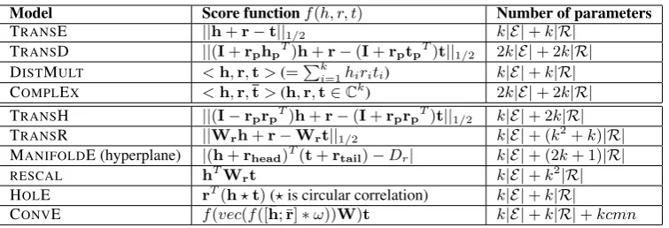
Model Score functionf(h, r, t) Number of parameters
TRANSE ||h+r−t||1/2 k|E|+k|R|
TRANSD ||(I+rphpT)h+r−(I+rptpT)t||1/2 2k|E|+ 2k|R| DISTMULT <h,r,t>(=Pki=1hiriti) k|E|+k|R| COMPLEX <h,r,¯t>(h,r,t∈Ck) 2k
|E|+ 2k|R| TRANSH ||(I−rprpT)h+r−(I+rprpT)t||1/2 k|E|+ 2k|R| TRANSR ||Wrh+r−Wrt||1/2 k|E|+ (k2+k)|R| MANIFOLDE (hyperplane) |(h+rhead)T(t+rtail)−Dr| k|E|+ (2k+ 1)|R|
RESCAL hTWrt k|E|+k2|R|
HOLE rT(h?t)(?is circular correlation) k|E|+k|R|
[image:2.595.112.490.60.189.2]CONVE f(vec(f([¯h; ¯r]∗ω))W)t k|E|+k|R|+kcmn
Table 1: Some selected knowledge graph embedding models. The four models above the double line are considered in this paper. Except for COMPLEX, all boldface lower case letters represent vectors inRk, and boldface upper case letters represent matrices inRk×k.Iis the identity matrix.
edge graph embedding models. Inspired by the recent advances of generative adversarial deep models (Goodfellow et al., 2014), we propose a novel adversarial learning framework, namely, KBGAN, for generating better negative exam-ples to train knowledge graph embedding mod-els. More specifically, we consider probability-based, log-loss embedding models as the gener-ator to supply better quality negative examples, and use distance-based, margin-loss embedding models as the discriminator to generate the final knowledge graph embeddings. Since the genera-tor has a discrete generation step, we cannot di-rectly use the gradient-based approach to back-propagate the errors. We then consider a one-step reinforcement learning setting, and use a variance-reductionREINFORCEmethod to achieve this goal. Empirically, we perform experiments on three common KGE datasets (FB15K-237, WN18 and WN18RR), and verify the adversarial learning approach with a set of KGE models. Our exper-iments show that across various settings, this ad-versarial learning mechanism can significantly im-prove the performance of some of the most com-monly used translation based KGE methods. Our contributions are three-fold:
• We are the first to consider adversarial learn-ing to generate useful negative trainlearn-ing exam-ples to improve knowledge graph embedding.
• This adversarial learning framework applies to a wide range of KGE models, without the need of external ontologies constraints.
• Our method shows consistent performance gains on three commonly used KGE datasets.
2 Related Work
2.1 Knowledge Graph Embeddings
A large number of knowledge graph embedding models, which represent entities and relations in a knowledge graph with vectors or matrices, have been proposed in recent years. RESCAL (Nickel et al., 2011) is one of the earliest studies on ma-trix factorization based knowledge graph embed-ding models, using a bilinear form as score func-tion. TRANSE (Bordes et al., 2013) is the first model to introduce translation-based embedding. Later variants, such as TRANSH (Wang et al., 2014), TRANSR (Lin et al., 2015) and TRANSD (Ji et al.,2015), extend TRANSE by projecting the embedding vectors of entities into various spaces. DISTMULT(Yang et al.,2015) simplifiesRESCAL by only using a diagonal matrix, and COMPLEX (Trouillon et al., 2016) extends DISTMULT into the complex number field. (Nickel et al.,2015) is a comprehensive survey on these models.
2.2 Generative Adversarial Networks and its Variants
Generative Adversarial Networks (GANs) (Good-fellow et al., 2014) was originally proposed for generating samples in a continuous space such as images. AGANconsists of two parts, the
genera-torand thediscriminator. The generator accepts a noise input and outputs an image. The discrimina-tor is a classifier which classifies images as “true” (from the ground truth set) or “fake” (generated by the generator). When training aGAN, the genera-tor and the discriminagenera-tor play a minimax game, in which the generator tries to generate “real” images to deceive the discriminator, and the discriminator tries to tell them apart from ground truth images. GANs are also capable of generating samples sat-isfying certain requirements, such as conditional GAN(Mirza and Osindero,2014).
It is not possible to useGANs in its original form for generating discrete samples like natural lan-guage sentences or knowledge graph triples, be-cause the discrete sampling step prevents gradi-ents from propagating back to the generator. SE -QGAN(Yu et al.,2017) is one of the first success-ful solutions to this problem by using reinforce-ment learning—It trains the generator using pol-icy gradient and other tricks.IRGAN(Wang et al., 2017) is a recent work which combines two cate-gories of information retrieval models into a dis-crete GAN framework. Likewise, our framework relies on policy gradient to train the generator which provides discrete negative triples.
The discriminator in a GAN is not necessarily a classifier. WassersteinGANorWGAN(Arjovsky et al.,2017) uses a regressor with clipped param-eters as its discriminator, based on solid analysis about the mathematical nature ofGANs. GOGAN (Juefei-Xu et al., 2017) further replaces the loss function in WGAN with marginal loss. Although originating from very different fields, the form of loss function in our framework turns out to be more closely related to the one in GOGAN. 3 Our Approaches
In this section, we first define two types of training objectives in knowledge graph embedding mod-els to show how KBGAN can be applied. Then, we demonstrate a long overlooked problem about negative sampling which motivates us to propose KBGAN to address the problem. Finally, we dive into the mathematical, and algorithmic details of
KBGAN.
3.1 Types of Training Objectives
For a given knowledge graph, let E be the set of entities, R be the set of relations, and T be the set of ground truth triples. In general, a knowledge graph embedding (KGE) model can be formulated as a score function f(h, r, t), h, t ∈ E, r ∈ R
which assigns a score to every possible triple in the knowledge graph. The estimated likelihood of a triple to be true depends only on its score given by the score function.
Different models formulate their score function based on different designs, and therefore interpret scores differently, which further lead to various training objectives. Two common forms of train-ing objectives are particularly of our interest: Marginal loss function is commonly used by a large group of models called translation-based models, whose score function models distance between points or vectors, such as TRANSE, TRANSH, TRANSR, TRANSD and so on. In these models, smaller distance indicates a higher likeli-hood of truth, but only qualitatively. The marginal loss function takes the following form:
Lm =
X
(h,r,t)∈T
[f(h, r, t)−f(h0, r, t0) +γ]+ (1)
where γ is the margin, [·]+ = max(0,·) is the
hinge function, and (h0, r, t0) is a negative triple.
The negative triple is generated by replacing the head entity or the tail entity of a positive triple with a random entity in the knowledge graph, or formally (h0, r, t0) ∈ {(h0, r, t)|h0 ∈ E} ∪
{(h, r, t0)|t0 ∈ E}.
Log-softmax loss functionis commonly used by models whose score function has probabilistic in-terpretation. Some notable examples areRESCAL, DISTMULT, COMPLEX. Applying the softmax function on scores of a given set of triples gives the probability of a triple to be the best one among them: p(h, r, t) = P expf(h,r,t)
(h0,r,t0)expf(h0,r,t0). The loss function is the negative log-likelihood of this prob-abilistic model:
Ll=
X
(h,r,t)∈T
−logPexpf(h, r, t)
expf(h0, r, t0)
(h0, r, t0)∈ {(h, r, t)} ∪N eg(h, r, t) (2)
where N eg(h, r, t) ⊂ {(h0, r, t)|h0 ∈ E} ∪
{(h, r, t0)|t0 ∈ E} is a set of sampled corrupted
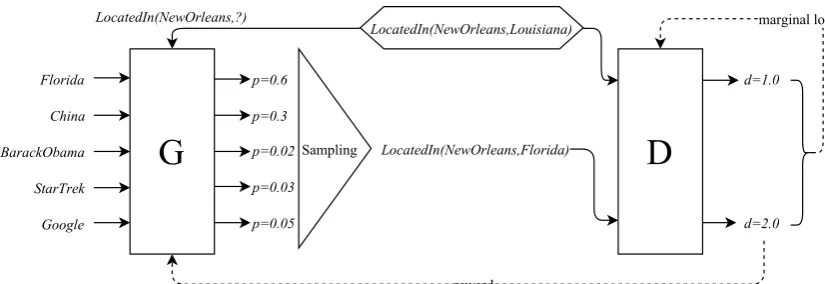
Figure 1: An overview of theKBGANframework. The generator (G) calculates a probability distribution over a set of candidate negative triples, then sample one triples from the distribution as the output. The discriminator (D) receives the generated negative triple as well as the ground truth triple (in the hexag-onal box), and calculates their scores. G minimizes the score of the generated negative triple by policy gradient, and D minimizes the marginal loss between positive and negative triples by gradient descent.
Other forms of loss functions exist, for exam-ple CONVE uses a triple-wise logistic function to model how likely the triple is true, but by far the two described above are the most common. Also, softmax function gives an probabilistic distribu-tion over a set of triples, which is necessary for a generator to sample from them.
3.2 Weakness of Uniform Negative Sampling Most previous KGE models useuniform negative samplingfor generating negative triples, that is, re-placing the head or tail entity of a positive triple with any of the entities in E, all with equal prob-ability. Most of the negative triples generated in this way contribute little to learning an effective embedding, because they are too obviously false.
To demonstrate this issue, let us consider the following example. Suppose we have a ground truth triple LocatedIn(NewOrleans,Louisiana), and corrupt it by replacing its tail entity. First, we remove the tail entity, leaving Lo-catedIn(NewOrleans,?). Because the relation Lo-catedIn constraints types of its entities, “?” must be a geographical region. If we fill “?” with a random entity e ∈ E, the
prob-ability of e having a wrong type is very
high, resulting in ridiculous triples like Lo-catedIn(NewOrleans,BarackObama) or Locate-dIn(NewOrleans,StarTrek). Such triples are con-sidered “too easy”, because they can be elim-inated solely by types. In contrast, Locate-dIn(NewOrleans,Florida)is a very useful negative triple, because it satisfies type constraints, but it cannot be proved wrong without detailed
knowl-edge of American geography. If a KGE model is fed with mostly “too easy” negative examples, it would probably only learn to represent types, not the underlying semantics.
The problem is less severe to models using log-softmax loss function, because they typically sam-ples tens or hundreds of negative trisam-ples for one positive triple in each iteration, and it is likely to have a few useful negatives among them. For in-stance, (Trouillon et al.,2016) found that a 100:1 negative-to-positive ratio results in the best per-formance for COMPLEX. However, for marginal loss function, whose negative-to-positive ratio is always 1:1, the low quality of uniformly sampled negatives can seriously damage their performance. 3.3 Generative Adversarial Training for Knowledge Graph Embedding Models
Inspired by GANs, we propose an adversarial training framework named KBGAN which uses a KGE model with softmax probabilities to pro-vide high-quality negative samples for the train-ing of a KGE model whose traintrain-ing objective is marginal loss function. This framework is inde-pendent of the score functions of these two mod-els, and therefore possesses some extent of univer-sality. Figure1 illustrates the overall structure of KBGAN.
distribu-Algorithm 1:TheKBGANalgorithm
Data:training set of positive fact triplesT ={(h, r, t)}
Input:Pre-trained generator G with parametersθGand score functionfG(h, r, t), and pre-trained discriminator D with parametersθDand score functionfD(h, r, t)
Output:Adversarially trained discriminator
1 b←−0;// baseline for policy gradient 2 repeat
3 Sample a mini-batch of dataTbatchfromT ;
4 GG←−0,GD←−0;// gradients of parameters of G and D
5 rsum←−0;// for calculating the baseline
6 for(h, r, t)∈ Tbatchdo
7 Uniformly randomly sampleNsnegative triplesN eg(h, r, t) ={(h0i, r, t0i)}i=1...Ns;
8 Obtain their probability of being generated:pi= expfG(h 0
i,r,t0i) PNs
j=1expfG(h0j,r,t0j)
;
9 Sample one negative triple(h0s, r, t0s)fromN eg(h, r, t)according to{pi}i=1...Ns. Assume its probability to be
ps;
10 GD←−GD+∇θD[fD(h, r, t)−fD(h0s, r, t0s) +γ]+;// accumulate gradients for D
11 r←− −fD(h0
s, r, t0s), rsum←−rsum+r;// r is the reward
12 GG←−GG+ (r−b)∇θGlogps;// accumulate gradients for G
13 end
14 θG←−θG+ηGGG, θD←−θD−ηDGD;// update parameters
15 b←rsum/|Tbatch|;// update baseline
16 untilconvergence;
tion” process of discrete GANs, and we aim at improving discriminators based on marginal loss because they can benefit more from high-quality negative samples. Note that a major difference be-tweenGANand our work is that, the ultimate goal of our framework is to produce a good discrimi-nator, whereasGANSare aimed at training a good generator. In addition, the discriminator here is not a classifier as it would be in mostGANs.
Intuitively, the discriminator should assign a rel-atively small distance to a high-quality negative sample. In order to encourage the generator to gen-erate useful negative samples, the objective of the generator is to minimize the distance given by dis-criminator for its generated triples. And just like the ordinary training process, the objective of the discriminator is to minimize the marginal loss be-tween the positive triple and the generated nega-tive triple. In an adversarial training setting, the generator and the discriminator are alternatively trained towards their respective objectives.
Suppose that the generator produces a probability distribution on negative triples
pG(h0, r, t0|h, r, t) given a positive triple(h, r, t), and generates negative triples (h0, r, t0) by
sam-pling from this distribution. Let fD(h, r, t) be the score function of the discriminator. The ob-jective of the discriminator can be formulated as
minimizing the following marginal loss function:
LD =
X
(h,r,t)∈T
[fD(h, r, t)−fD(h0, r, t0) +γ]+
(h0, r, t0)∼pG(h0, r, t0|h, r, t) (3)
The only difference between this loss function and Equation1is that it uses negative samples from the generator.
The objective of the generator can be formu-lated as maximizing the following expectation of negative distances:
RG=
X
(h,r,t)∈T
E[−fD(h0, r, t0)]
(h0, r, t0)∼pG(h0, r, t0|h, r, t) (4)
RG involves a discrete sampling step, so we cannot find its gradient with simple differentiation. We use a simple special case of Policy Gradient Theorem1(Sutton et al.,2000) to obtain the gradi-ent ofRGwith respect to parameters of the gener-ator:
∇GRG=
X
(h,r,t)∈T
E(h0,r,t0)∼pG(h0,r,t0|h,r,t)
[−fD(h0, r, t0)∇GlogpG(h0, r, t0|h, r, t)]
' X
(h,r,t)∈T
1 N
X
(h0
i,r,t0i)∼pG(h0,r,t0|h,r,t),i=1...N
[−fD(h0, r, t0)∇GlogpG(h0, r, t0|h, r, t)] (5)
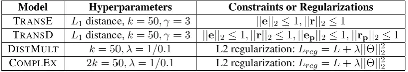
Model Hyperparameters Constraints or Regularizations TRANSE L1distance,k= 50, γ= 3 ||e||2 ≤1,||r||2 ≤1
TRANSD L1distance,k= 50, γ= 3 ||e||2≤1,||r||2≤1,||ep||2 ≤1,||rp||2 ≤1
DISTMULT k= 50, λ= 1/0.1 L2 regularization:Lreg =L+λ||Θ||22
COMPLEX 2k= 50, λ= 1/0.1 L2 regularization:Lreg =L+λ||Θ||22
Table 2: Hyperparameter settings of the 4 models we used. For DISTMULT and COMPLEX,λ = 1is
used for FB15k-237 andλ= 0.1is used for WN18 and WN18RR. All other hyperparameters are shared
among all datasets.Lis the global loss defined in Equation (2).Θrepresents all parameters in the model.
Dataset #r #ent. #train #val #test
[image:6.595.97.502.62.134.2]FB15k-237 237 14,541 272,115 17,535 20,466 WN18 18 40,943 141,442 5,000 5,000 WN18RR 11 40,943 86,835 3,034 3,134 Table 3: Statistics of datasets we used in the exper-iments. “r”: relations.
where the second approximate equality means we approximate the expectation with sampling in practice. Now we can calculate the gradient ofRG and optimize it with gradient-based algorithms.
Policy Gradient Theorem arises from reinforce-ment learning (RL), so we would like to draw an analogy between our model and an RL model. The generator can be viewed as anagentwhich inter-acts with the environment by performingactions
and improves itself by maximizing thereward re-turned from the environment in response of its ac-tions. Correspondingly, the discriminator can be viewed as the environment. Using RL terminolo-gies, (h, r, t)is the state(which determines what
actions the actor can take), pG(h0, r, t0|h, r, t) is thepolicy(how the actor choose actions),(h0, r, t0)
is the action, and −fD(h0, r, t0) is the reward. The method of optimizing RG described above is called REINFORCE (Williams,1992) algorithm in RL. Our model is a simple special case of RL, called one-step RL. In a typical RL setting, each action performed by the agent will change its state, and the agent will perform a series of actions (called an epoch) until it reaches certain states or the number of actions reaches a certain limit. However, in the analogy above, actions does not affect the state, and after each action we restart with another unrelated state, so each epoch con-sists of only one action.
To reduce the variance of REINFORCE al-gorithm, it is common to subtract a base-line from the reward, which is an arbitrary number that only depends on the state,
with-out affecting the expectation of gradients.2 In our case, we replace −fD(h0, r, t0) with −fD(h0, r, t0) − b(h, r, t) in the equation above to introduce the baseline. To avoid introducing new parameters, we simply let b be a constant,
the average reward of the whole training set:b = P
(h,r,t)∈T E(h0,r,t0)∼pG(h0,r,t0|h,r,t)[−fD(h0, r, t0)]. In practice, b is approximated by the mean of
rewards of recently generated negative triples. Let the generator’s score function to be
fG(h, r, t), given a set of candidate negative triples
N eg(h, r, t)⊂ {(h0, r, t)|h0 ∈ E}∪{(h, r, t0)|t0∈
E}, the probability distributionpGis modeled as:
pG(h0, r, t0|h, r, t) =
expfG(h0, r, t0)
P
expfG(h∗, r, t∗)
(h∗, r, t∗)∈N eg(h, r, t) (6)
Ideally,N eg(h, r, t)should contain all possible
negatives. However, knowledge graphs are usu-ally highly incomplete, so the ”hardest” negative triples are very likely to be false negatives (true facts). To address this issue, we instead generate
N eg(h, r, t)by uniformly sampling ofNsentities (a small number compared to the number of all possible negatives) fromE to replace h ort.
Be-cause in real-world knowledge graphs, true neg-atives are usually far more than false negneg-atives, such set would be unlikely to contain any false negative, and the negative selected by the gener-ator would likely be a true negative. Using a small
N eg(h, r, t)can also significantly reduce
compu-tational complexity.
Besides, we adopt the “bern” sampling tech-nique (Wang et al., 2014) which replaces the “1” side in “1-to-N” and “N-to-1” relations with higher probability to further reduce false nega-tives.
criminator require pre-training, which is the same as conventionally training a single KBE model with uniform negative sampling. Formally speak-ing, one can pre-train the generator by minimiz-ing the loss function defined in Equation (1), and pre-train the discriminator by minimizing the loss function defined in Equation (2). Line 14 in the algorithm assumes that we are using the vanilla gradient descent as the optimization method, but obviously one can substitute it with any gradient-based optimization algorithm.
4 Experiments
To evaluate our proposed framework, we test its performance for the link prediction task with dif-ferent generators and discriminators. For the gen-erator, we choose two classical probability-based KGE model, DISTMULT and COMPLEX, and for the discriminator, we also choose two classi-cal translation-based KGE model, TRANSE and TRANSD, resulting in four possible combinations of generator and discriminator in total. See Table 1for a brief summary of these models.
4.1 Experimental Settings 4.1.1 Datasets
We use three common knowledge base com-pletion datasets for our experiment: FB15k-237, WN18 and WN18RR. FB15k-237 is a subset of FB15k introduced by (Toutanova and Chen, 2015), which removed redundant relations in FB15k and greatly reduced the number of rela-tions. Likewise, WN18RR is a subset of WN18 in-troduced by (Dettmers et al.,2017) which removes reversing relations and dramatically increases the difficulty of reasoning. Both FB15k and WN18 are first introduced by (Bordes et al., 2013) and have been commonly used in knowledge graph re-searches. Statistics of datasets we used are shown in Table3.
4.1.2 Evaluation Protocols
Following previous works like (Yang et al.,2015) and (Trouillon et al., 2016), for each run, we re-port two common metrics, mean reciprocal rank-ing (MRR) and hits at 10 (H@10). We only re-port scores under thefilteredsetting (Bordes et al., 2013), which removes all triples appeared in train-ing, validattrain-ing, and testing sets from candidate triples before obtaining the rank of the ground truth triple.
4.1.3 Implementation Details
3 In the pre-training stage, we train every model to convergence for 1000 epochs, and divide ev-ery epoch into 100 mini-batches. To avoid overfit-ting, we adopt early stopping by evaluating MRR on the validation set every 50 epochs. We tried
γ = 0.5,1,2,3,4,5 and L1, L2 distances for
TRANSE and TRANSD, andλ = 0.01,0.1,1,10
for DISTMULT and COMPLEX, and determined the best hyperparameters listed on table2, based on their performances on the validation set af-ter ptraining. Due to limited computation re-sources, we deliberately limit the dimensions of embeddings to k = 50, similar to the one used
in earlier works, to save time. We also apply cer-tain constraints or regularizations to these models, which are mostly the same as those described in their original publications, and also listed on table 2.
In the adversarial training stage, we keep all the hyperparamters determined in the pre-training stage unchanged. The number of candidate neg-ative triples, Ns, is set to 20 in all cases, which
is proven to be optimal among the candidate set of {5,10,20,30,50}. We train for 5000 epochs,
with 100 mini-batches for each epoch. We also use early stopping in adversarial training by evaluating MRR on the validation set every 100 epochs.
We use the self-adaptive optimization method Adam (Kingma and Ba, 2015) for all trainings, and always use the recommended default setting
α= 0.001, β1 = 0.9, β2 = 0.999, = 10−8.
4.2 Results
Results of our experiments as well as baselines are shown in Table 4. All settings of adversarial training bring a pronounced improvement to the model, which indicates that our method is con-sistently effective in various cases. TRANSE per-forms slightly worse than TRANSD on FB15k-237 and WN18, but better on WN18RR. Using DIST -MULTor COMPLEXas the generator does not af-fect performance greatly.
TRANSE and TRANSD enhanced by KBGAN can significantly beat their corresponding baseline implementations, and outperform stronger base-lines in some cases. As a prototypical and proof-of-principle experiment, we have never expected state-of-the-art results. Being simple models
pro-3The KBGAN source code is available at https://
FB15k-237 WN18 WN18RR
Method MRR H@10 MRR H@10 MRR H@10
TRANSE - 42.8† - 89.2 - 43.2†
TRANSD - 45.3† - 92.2 - 42.8†
[image:8.595.106.496.61.227.2]DISTMULT 24.1‡ 41.9‡ 82.2 93.6 42.5‡ 49.1‡ COMPLEX 24.0‡ 41.9‡ 94.1 94.7 44.4‡ 50.7‡ TRANSE (pre-trained) 24.2 42.2 43.3 91.5 18.6 45.9 KBGAN(TRANSE + DISTMULT) 27.4 45.0 71.0 94.9 21.3 48.1 KBGAN(TRANSE + COMPLEX) 27.8 45.3 70.5 94.9 21.0 47.9 TRANSD (pre-trained) 24.5 42.7 49.4 92.8 19.2 46.5 KBGAN(TRANSD + DISTMULT) 27.8 45.8 77.2 94.8 21.4 47.2 KBGAN(TRANSD + COMPLEX) 27.7 45.8 77.9 94.8 21.5 46.9
Table 4: Experimental results. Results of KBGANare results of its discriminator (on the left of the “+” sign). Underlined results are the best ones among our implementations. Results marked with†are pro-duced by running Fast-TransX (Lin et al.,2015) with its default parameters. Results marked with‡are copied from (Dettmers et al.,2017). All other baseline results are copied from their original papers.
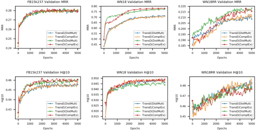
Figure 2: Learning curves ofKBGAN. All metrics improve steadily as training proceeds.
posed several years ago, TRANSE and TRANSD has their limitations in expressiveness that are un-likely to be fully compensated by better training technique. In future researches, people may try employing more advanced models into KBGAN, and we believe it has the potential to become state-of-the-art.
To illustrate our training progress, we plot per-formances of the discriminator on validation set over epochs, which are displayed in Figure2. As all these graphs show, our performances are al-ways in increasing trends, converging to its
[image:8.595.78.524.317.543.2]Positive fact Uniform random sample Trained generator (condensation NN 2,
derivationally related form, distill VB 4)
family arcidae NN 1 repast NN 1
beater NN 2 coverall NN 1 cash advance NN 1
revivification NN 1 mouthpiece NN 3
liquid body substance NN 1
stiffen VB 2
hot up VB 1
(colorado river NN 2, instance hypernym, river NN 1)
lunar calendar NN 1
umbellularia californica NN 1 tonality NN 1
creepy-crawly NN 1 moor VB 3
idaho NN 1
sayan mountains NN 1 lower saxony NN 1
order ciconiiformes NN 1 jab NN 3
(meeting NN 2, hypernym,
social gathering NN 1)
cellular JJ 1
commercial activity NN 1 giant cane NN 1
streptomyces NN 1 tranquillize VB 1
attach VB 1 bond NN 6
[image:9.595.77.520.63.280.2]heavy spar NN 1 satellite NN 1 peep VB 3
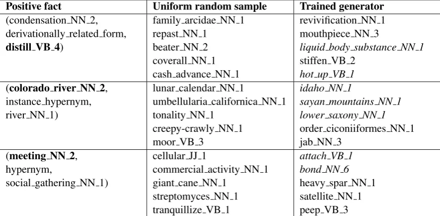
Table 5: Examples of negative samples in WN18 dataset. The first column is the positive fact, and the term in bold is the one to be replaced by an entity in the next two columns. The second column consists of random entities drawn from the whole dataset. The third column contains negative samples generated by the generator in the last 5 epochs of training. Entities in italic are considered to have semantic relation to the positive one
4.3 Case study
To demonstrate that our approach does generate better negative samples, we list some examples of them in Table 5, using the KBGAN (TRANSE + DISTMULT) model and the WN18 dataset. All hy-perparameters are the same as those described in Section 4.1.3.
Compared to uniform random negatives which are almost always totally unrelated, the genera-tor generates more semantically related negative samples, which is different from type relatedness we used as example in Section 3.2, but also helps training. In the first example, two of the five terms are physically related to the process of distilling liquids. In the second example, three of the five entities are geographical objects. In the third ex-ample, two of the five entities express the concept of “gather”.
Because we deliberately limited the strength of generated negatives by using a small Ns as de-scribed in Section 3.3, the semantic relation is pretty weak, and there are still many unrelated en-tities. However, empirical results (when selecting the optimalNs) shows that such situation is more
beneficial for training the discriminator than gen-erating even stronger negatives.
5 Conclusions
References
Martin Arjovsky, Soumith Chintala, and Leon Bottou. 2017. Wasserstein gan. In International Confer-rence on Machine Learning.
Kurt Bollacker, Colin Evans, Praveen Paritosh, Tim Sturge, and Jamie Taylor. 2008. Freebase: a collab-oratively created graph database for structuring hu-man knowledge. In Proceedings of the 2008 ACM SIGMOD international conference on Management of data. ACM, pages 1247–1250.
Antoine Bordes, Nicolas Usunier, Alberto Garcia-Duran, Jason Weston, and Oksana Yakhnenko. 2013. Translating embeddings for modeling multi-relational data. InAdvances in Neural Information Processing Systems. pages 2787–2795.
Tim Dettmers, Pasquale Minervini, Pontus Stene-torp, and Sebastian Riedel. 2017. Convolutional 2d knowledge graph embeddings. arXiv preprint arXiv:1707.01476.
Xin Dong, Evgeniy Gabrilovich, Geremy Heitz, Wilko Horn, Ni Lao, Kevin Murphy, Thomas Strohmann, Shaohua Sun, and Wei Zhang. 2014. Knowledge vault: A web-scale approach to probabilistic knowl-edge fusion. In Proceedings of the 20th ACM SIGKDD international conference on Knowledge discovery and data mining. ACM, pages 601–610. Ian Goodfellow, Jean Pouget-Abadie, Mehdi Mirza,
Bing Xu, David Warde-Farley, Sherjil Ozair, Aaron Courville, and Yoshua Bengio. 2014. Generative ad-versarial nets. In Advances in Neural Information Processing Systems. pages 2672–2680.
Guoliang Ji, Shizhu He, Liheng Xu, Kang Liu, and Jun Zhao. 2015. Knowledge graph embedding via dy-namic mapping matrix. InThe 53rd Annual Meeting of the Association for Computational Linguistics. Felix Juefei-Xu, Vishnu Naresh Boddeti, and Marios
Savvides. 2017. Gang of gans: Generative adversar-ial networks with maximum margin ranking. arXiv preprint arXiv:1704.04865.
Diederik P. Kingma and Jimmy Lei Ba. 2015. Adam: A method for stochastic optimization. In The 3rd International Conference on Learning Representa-tions.
Denis Krompaß, Stephan Baier, and Volker Tresp. 2015. Type-constrained representation learning in knowledge graphs. InInternational Semantic Web Conference. Springer, pages 640–655.
Yankai Lin, Zhiyuan Liu, Maosong Sun, Yang Liu, and Xuan Zhu. 2015. Learning entity and relation em-beddings for knowledge graph completion. InThe Twenty-ninth AAAI Conference on Artificial Intelli-gence. pages 2181–2187.
Mehdi Mirza and Simon Osindero. 2014. Condi-tional generative adversarial nets. arXiv preprint arXiv:1411.01784.
Tom M Mitchell, William Cohen, Estevam Hruschka, Partha Talukdar, Justin Betteridge, Andrew Carlson, Bhavana Dalvi Mishra, Matthew Gardner, Bryan Kisiel, Jayant Krishnamurthy, et al. 2015. Never-ending learning. InThe Twenty-ninth AAAI Confer-ence on Artificial IntelligConfer-ence.
Maximilian Nickel, Kevin Murphy, Volker Tresp, and Evgeniy Gabrilovich. 2015. A review of relational machine learning for knowledge graphs. arXiv preprint arXiv:1503.00759.
Maximilian Nickel, Lorenzo Rosasco, and Tomaso Poggio Poggio. 2016. Holographic embeddings of knowledge graphs. InThe Thirtieth AAAI Conference on Artificial Intelligence. pages 1955–1961.
Maximilian Nickel, Volker Tresp, and Hans-Peter Kriegel. 2011. A three-way model for collective learning on multi-relational data. In Proceedings of the 28th International Conference on Machine Learning. pages 809–816.
Fabian M Suchanek, Gjergji Kasneci, and Gerhard Weikum. 2007. Yago: a core of semantic knowl-edge. InProceedings of the 16th international con-ference on World Wide Web. ACM, pages 697–706.
Richard S Sutton, David A McAllester, Satinder P Singh, and Yishay Mansour. 2000. Policy gradi-ent methods for reinforcemgradi-ent learning with func-tion approximafunc-tion. InAdvances in neural informa-tion processing systems. pages 1057–1063.
Kristina Toutanova and Danqi Chen. 2015. Observed versus latent features for knowledge base and text inference. InProceedings of the 3rd Workshop on Continuous Vector Space Models and their Compo-sitionality. pages 57–66.
Th´eo Trouillon, Johannes Welbl, Sebastian Riedel, ´Eric Gaussier, and Guillaume Bouchard. 2016. Com-plex embeddings for simple link prediction. In In-ternational Conference on Machine Learning. pages 2071–2080.
Jun Wang, Lantao Yu, Weinan Zhang, Yu Gong, Yinghui Xu, Benyou Wang, Peng Zhang, and Dell Zhang. 2017. Irgan: A minimax game for unifying generative and discriminative information retrieval models. InThe 40th International ACM SIGIR Con-ference.
Zhen Wang, Jianwen Zhang, Jianlin Feng, and Zheng Chen. 2014. Knowledge graph embedding by trans-lating on hyperplanes. InThe Twenty-eighth AAAI Conference on Artificial Intelligence. pages 1112– 1119.
Han Xiao, Minlie Huang, and Xiaoyan Zhu. 2016. From one point to a manifold: Knowledge graph em-bedding for precise link prediction. InThe Twenty-Fifth International Joint Conference on Artificial In-telligence.
Bishan Yang, Wen-tau Yih, Xiaodong He, Jianfeng Gao, and Li Deng. 2015. Embedding entities and relations for learning and inference in knowledge bases. The 3rd International Conference on Learn-ing Representations.